Development of process control strategies exploiting knowledge from systems biology: Application to MDCK suspension cells

(1)

Sheila Azim Piarali

Licenciada em Bioquímica

Development of process control

strategies exploiting knowledge from

systems biology: Application to MDCK

suspension cells

Dissertação para obtenção do Grau de Mestre em Biotecnologia

Orientador:

Dr. Moritz von Stosch, Postdoctoral Researcher, FCT-UNL

Co-orientadores:

PD Dr. Yvonne Genzel, Senior Scientist, MPI

Dr. Rui M. Freitas Oliveira, Associate Professor, FCT-UNL

Júri:

Presidente: Dr. Carlos Alberto Gomes Salgueiro

Vogais: Dra. Ana Margarida Palma Teixeira

Dr. Moritz von Stosch

(2)

(3)

iii Development of process control strategies exploiting knowledge from systems biology: Application to MDCK suspension cells

(4)

iv

ACKNOWLEDGEMENTS

Choosing Systems Biology as the theme of my Master thesis was indeed a challenge and overcoming it would not have been possible if I did not have Dr. Moritz von Stosch as my supervisor.

I want to thank him for his patience, for his will in seeing others succeed, for his kindness and for believing in me.

Also I would like to thank PD Dr. Yvonne Genzel for integrating me at the Max Planck Institute, for always showing availability and for her wise advices.

To my friend Tiago Costa who spent several hours instructing me, supporting me and giving me strength to continue my work.

To my colleagues, João Ramos and André Guerra for the great company throughout these months.

(5)

v

ABSTRACT

Madine Darby Canine Kidney (MDCK) cell lines have been extensively evaluated for their potential as host cells for influenza vaccine production. Recent studies allowed the cultivation of these cells in a fully defined medium and in suspension. However, reaching high cell densities in animal cell cultures still remains a challenge.

To address this shortcoming, a combined methodology allied with knowledge from systems biology was reported to study the impact of the cell environment on the flux distribution. An optimization of the medium composition was proposed for both a batch and a continuous system in order to reach higher cell densities. To obtain insight into the metabolic activity of these cells, a detailed metabolic model previously developed by Wahl A. et. al was used. The experimental data of four cultivations of MDCK suspension cells, grown under different conditions and used in this work came from the Max Planck Institute, Magdeburg, Germany.

Classical metabolic flux analysis (MFA) was used to estimate the intracellular flux distribution of each cultivation and then combined with partial least squares (PLS) method to establish a link between the estimated metabolic state and the cell environment. The validation of the MFA model was made and its consistency checked. The resulted PLS model explained almost 70% of the variance present in the flux distribution.

The medium optimization for the continuous system and for the batch system resulted in higher biomass growth rates than the ones obtained experimentally, 0.034 h -1_{and 0.030 h}-1_{, respectively, thus reducing in almost 10 hours the duplication time.}

Additionally, the optimal medium obtained for the continuous system almost did not consider pyruvate.

(6)

vi

RESUMO

Nos últimos tempos, o uso de linhas celulares de Madine Darby Canine Kidney (MDCK) em culturas de células animais tem sido extensivamente explorado devido ao seu potencial como células hospedeiras para a produção de vacinas contra a gripe. Estudos recentes permitiram o cultivo destas células num meio totalmente definido e em suspensão. No entanto, um dos desafios que se mantém é o de atingir elevadas densidades celulares.

De maneira a ultrapassar esta barreira, procedeu-se a uma combinação de metodologias e a conhecimentos de biologia de sistemas de modo a estudar-se o impacto do ambiente da célula nos fluxos intracelulares. Duas otimizações de meios de cultura foram propostas, quer para um sistema contínuo quer para um sistema descontínuo, a fim de se alcançarem densidades celulares mais elevadas.

Para obter um conhecimento mais detalhado sobre a atividade metabólica das células, o presente estudo baseou-se num modelo metabólico desenvolvido por Wahl et. al. Os dados experimentais de quatro culturas de células de MDCK em suspensão foram fornecidos pelo Max Plank Institute, Magdeburgo, Alemanha.

Metabolic flux analysis (MFA) foi utilizado para estimar os fluxos intracelulares e, posteriormente combinado com o Partial least squares (PLS) para estabelecer uma ligação entre o estado metabólico estimado e o ambiente extracelular da célula. A validação do modelo de MFA foi feita bem como a análise da sua consistência. O modelo de PLS resultou na explicação de cerca de 70% de variância para a distribuição de fluxos intracelulares.

Ambas as otimizações resultaram em taxas de crescimento mais elevadas que as obtidas experimentalmente, reduzindo em cerca de 10h o tempo de duplicação. A otimização para o sistema contínuo resultou ainda num meio sem piruvato.

(7)

vii

LIST OF FIGURES

Figure 1. Concentration profiles over time for Lactate excretion during the exponential phase. The solid lines represent the model fit. The first cultivation is represented by dark blue, the second cultivation is represented by red, the third cultivation is represented by yellow and the fourth cultivation is represented by light blue. ... 6

Figure 2. Schematic representation of Metabolic Flux Analysis first steps to calculate intracellular fluxes. (A) Development of a metabolic network of a certain system, (B) Formulation of the respective material balance equations for each metabolite present in the model, (C) Creation of a stoichiometric matrix based on stoichiometric coefficients, (D) Representation of the resulting data into a matrix form. ... 7

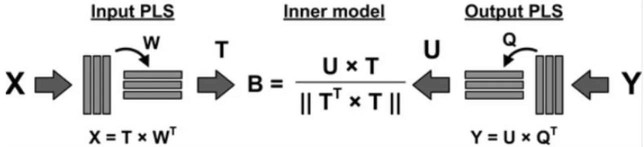
Figure 3. Schematic representation of PLS model. Left side represents the independent variables or inputs and the right side represents the dependent variables or outputs. Both sets of variables are decomposed into scores, T and U, and loadings, W and Q. The scores are then regressed against each other resulting in a diagonal matrix with the regression coefficients, B (adapted from Ferreira et al. [48]). ... 11

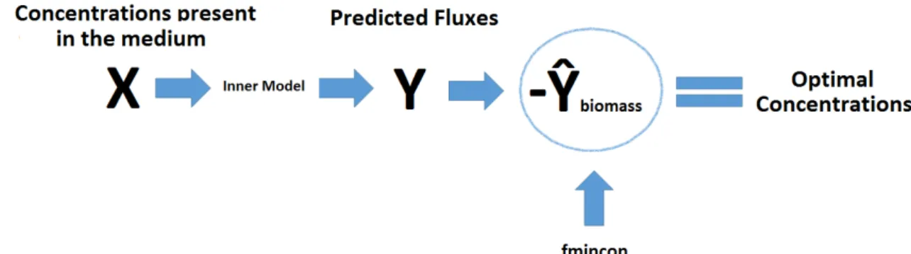
Figure 4. After the selection of the inputs through the PLS model, new predictions were made. Being the biomass growth rate, the rate of interest a mathematical maximization function, fmincon (MATLAB, the Mathworks, 2013) was applied in order to determine the optimal medium concentrations that resulted in a maximization of the biomass growth rate. ... 12

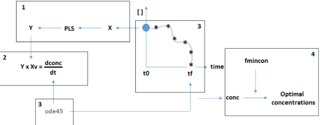
Figure 5. Given a specific set of concentrations, X, previously calculated by the PLS model a new PLS is applied and new fluxes are calculated, Y. (2) By multiplying the new fluxes with the biomass we obtain the derivatives of the concentrations. (3) Using solver function ode45, integrals are calculated from t0 to tf and as a result, concentration values are obtained for every time point. (4) Given the biomass concentration, fmincon is applied in order to determine the optimal concentrations that maximize the biomass growth. . 13

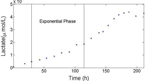
Figure 6. Concentration profile of Lactate excretion over time for Cultivation 1. Solid lines represent the time range defined. ... 14

Figure 7. First steps applied in the medium concentrations in order to calculate the extracellular fluxes. ... 14

(10)

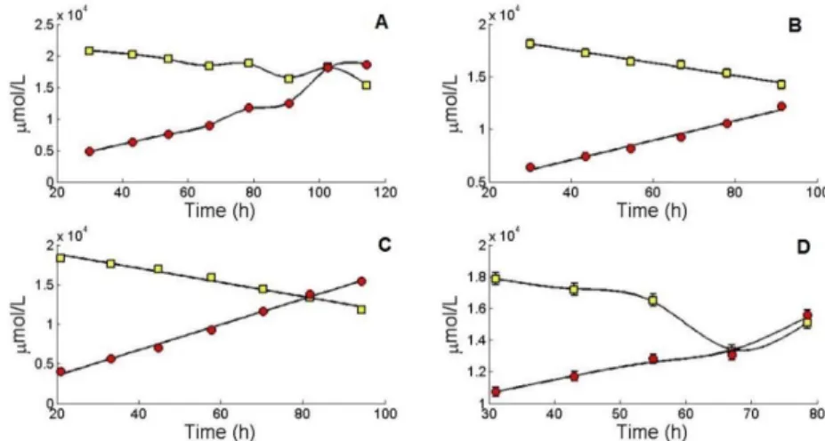
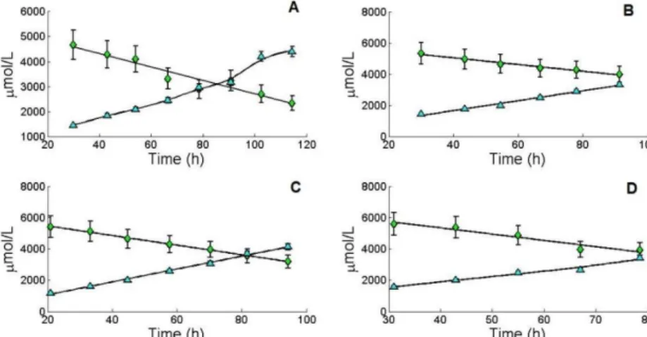
x Figure 9. Concentration values for ammonia release and glutamine uptake during the exponential phase of MDCK suspension cells with respective standard deviations. (A) Represents the first cultivation; (B) represents the second cultivation; (C) represents the third cultivation; (D) represents the fourth cultivation; gln ( ), NH3 ( ). ... 16

Figure 10. Concentration values for the uptake of pyruvate during the exponential phase of MDCK suspension cells. Dark blue represents the first cultivation; red represents the second cultivation; light blue represents the fourth cultivation. ... 16

Figure 11. Biomass concentration during the exponential phase of MDCK suspension cells for all cultivations. The solid lines represent the model fit. Cultivation 1 is represented in dark blue and has a final cell density of 9.24 g/L; Cultivation 2 is represented in red and has a final cell density of 8.88 g/L; Cultivation 3 is represented in yellow and has a final cell density of 11.50 g/L; Cultivation 4 is represented by light blue and has a final cell density of 8.28 g/L. ... 17

Figure 12. Overview of all the steps performed in the experimental data in order to evaluate the cell metabolism. ... 18

Figure 13. Consistency index (h) over time for each cultivation with test function (χ2 (0.95, 8) = 15.50). (A) Cultivation 1; (B) Cultivation 2; (C) Cultivation 3; (D) Cultivation 4. ... 23

Figure 14. Metabolic flux distribution for all cultivations. (A) Cultivation 1; (B) Cultivation 2; (C) Cultivation 3; (D) Cultivation 4. ... 24

Figure 15. Modelling error obtained for each LV with single cross validation technique for the validation set. ... 25

Figure 16. Correlation between predicted fluxes and measured fluxes. ... 27

Figure 17. Prediction of the specific biomass growth rate (µ). Solid blue line represents the measured flux and solid black line represents the predicted flux. ... 27

Figure 18. 2D score plot and 3D score plot from the PLS model. Cultivation 1 is represented in dark blue; Cultivation 2 is represented in red; Cultivation 3 is represented in yellow and; Cultivation 4 is represented in light blue. ... 28

(11)

xi Figure 20. Elasticities of each intracellular flux with respect to each compound present in the medium for the final time point for all cultivations (order of representation C1, C2, C3 and C4). ... 32

Figure 21. Elasticity for the biomass growth rate with respect to each component at the initial time point (left) and the final time point (right). ... 33

Figure 22. Pathway regulation by glucose, pyruvate, methionine and histidine for C1. 33 Figure 23 X loadings and Y loadings for 3 latent variables. (1) Gln, (2) NH3, (3) Glc, (4) Lac, (5) Glu, (6) Pyr, (7) Arg, (8) Asn, (9) Ala, (10) Thr, (11) Gly, (12) Val, (13) Ile, (14) Leu, (15) Met, (16) His, (17) Phe, (18) Asp, (19) Cys, (20) Tyr, 21 (Trp). ... 34

Figure 24. Optimal concentration for the continuous optimization. ... 35

Figure 25. Initial optimal concentration for the batch optimization. ... 35

Figure 26. Comparison between the optimal concentrations obtained for the continuous system and the initial optimal concentrations for the batch system. ... 36

(12)

xii

LIST OF TABLES

Table 1. Cultivations considered for MFA and PLS modeling ... 4

Table 2. Smoothing parameters attributed for each compound present on each cultivation ... 5

Table 3. Final cell density (g/L), biomass growth rate (h-1) and duplication time (h) for all cultivations during the exponential phase. ... 18

Table 4. Average extracellular fluxes (µmol/cell/h) and respective standard deviations calculated using a Monte Carlo approach during the time range considered for each cultivation. ... 19

Table 5. Average intracellular fluxes estimated by MFA (µmol/cell/h) during the time range considered for each cultivation. ... 20

Table 6. Training model decomposition results in terms of % of explained variance over number of latent variables. ... 26

Table 7. PLS model decomposition results in terms of % of explained variance over number of latent variables. ... 26

Table 8. Comparison of the biomass growth rates (h-1_{) and duplication time (h) obtained}

experimentally and with the batch and continuous optimizations. ... 35

Table 9. Comparison between the average experimental concentrations used in the cultivations and the optimal concentrations obtained for the continuous optimization and batch optimization (µmol/L). ... 37

(13)

xiii

ACRONYMS

MDCK – Madine Darby Canine Kidney

MFA – Metabolic Flux Analysis

PLS – Partial Least Squares

Gln - Glutamine

NH3 - Ammonia

Glc - Glucose

Lac- Lactate

Glu- Glutamate

Pyr - Pyruvate

Arg - Arginine

Asn - Asparagine

Ala - Alanine

Thr - Threonine

Gly - Glycine

Val - Valine

Ser - Serine

Pro - Proline

Ile - Isoleucine

Leu - Leucine

Met - Methionine

His - Histidine

Phe - Phenylalanine

Asp - Aspartate

Cys - Cysteine

Tyr - Tyrosine

Trp – Tryptophan

TCA – Tricarboxylic acid

(14)

xiv DNA – Deoxyribonucleic acid

RNA – Ribonucleic acid

WLS – Weighted Least Squares

LV – Latent variables

X – Independent variables

Y – Dependent variables

T – Scores for the independent variables

U – Scores for the dependent variables

W – Loadings for the independent variables

Q – Scores for the dependent variables

B – Regression coefficient matrix

C1 – Cultivation 1

(15)

(16)

1

Introduction

Influenza constitutes a serious threat to public health. According to sources [1-4], seasonal influenza epidemics affect between 5 and 15% of the world population causing cases of severe illness and about 500.000 deaths every year. The probability that a pandemic influenza outbreak occurs and the concern that comes with it, has led to intensive efforts in the scientific community to increase the production of influenza vaccines [5-7].

Although many alternatives have been developed to control diseases caused by the influenza virus, vaccination remains the most effective prevention strategy [3, 5, 8]. However, antigenic shifts of the virus occur frequently, wherefore new vaccines are needed every season [3, 9]. It takes 3-4 months to prepare a suitable vaccine if a high seed virus is available, whereas the pandemic only takes approximately 3 months for spreading through all continents [6]. Therefore, the development of the vaccine manufacturing process must yield a fast process, which ensures constant high-quality in large quantities.

The traditional approach to produce vaccines against influenza virus uses embryonated chicken eggs [3, 5, 6, 8, 10]. This approach presents considerable drawbacks [11]. For instance, several months are needed to produce chicken flocks capable of producing embryonated eggs. Different studies have also shown that the composition of hemagglutinin changes when the virus is passed to the chicken eggs, leading to: 1) undesired immune responses; 2) the need of an extensive manufacturing control throughout the process due to the inherent microbial burden in eggs; and 3) the difficulties associated with the scale-up processing in a short period of time [4, 8, 12].

Over the past years, a main focus consisted in developing cell culture systems for influenza virus replication. Many cell lines, like African Green Monkey (Vero) and Madine Darby Canine Kidney (MDCK) cells, have been proposed as host cells for influenza vaccine production. Both of these mammalian cell lines can yield high virus titers, show good reproduction of influenza strains and similar characteristics [3, 5, 11-13].

In this study, we focus on MDCK cells. MDCK cells can grow in suspension, which brings more benefits in terms of production costs when compared to adherent cells, due to the elimination of complex processing steps associated with microcarriers [8, 14]. Additionally, these cells have been reported to grow on chemically defined culture media, which diminishes batch-to-batch variations and the risk of contaminations. MDCK cells are also resistant to the toxic effects of trypsin supplementation and, as described before, they are highly permissive for propagation of influenza viruses [1, 7, 10, 11, 15].

During MDCK cultivations, four characteristic process phases are distinguished, namely adaptation phase, exponential growth phase, inhibition phase and confluent phase. During the adaptation or “lag” phase cells are not growing because they are adapting to the culture conditions. In the exponential growth phase the cells grow at maximum specific growth rate. The inhibition phase results in the decrease of the specific growth rate and finally in the confluent phase the specific growth rate approaches to zero due to the lack of nutrients [16].

(17)

2 (number of cells per unit volume) is observed. The infected cells start to produce virus particles, which first accumulate inside the cells and then start budding from the host cells. The released virions then infect other cells, which have been uninfected to this stage. The produced virus can then be separated from the cells/culture by chromatography [2, 13, 17].

Despite having a cell line that can grow in suspension and the respective techniques to isolate the virus, infect the host cells and collect the final product, one of the main challenges that still remains is to ensure high influenza yields and good quality in a short period of time.

One way to overcome this problem is to increase the yield in high cell density cultures. As mentioned before, cell density represents the number of cells per unit volume. In theory, the higher the cell density, the higher the amount of cells per unit volume, therefore more cells are available to be infected at time of infection leading to high virus titers in less time. Distinct strategies are used to reach high cell densities such as genetic modifications of the host cells, improvement of the medium composition and control and analysis of the process [18].

Notwithstanding the existing strategies there are problems that appear when in high cell density conditions that still remain unsolved. For example, it has been observed that from a certain density, the cells start to slow down their growth even though a high number of cells is present in the culture, the so called high cell density effect which was also reported for insect cell lines [6, 19, 20]. In this scenario, specific rates of glucose and glutamine consumption decrease significantly and also apoptosis occurs [9]. It is assumed by many that this effect is due to depletion of nutrients; accumulation of toxic compounds; cell-to-cell contact [18, 21]. Yet, what actually causes it still is not completely known.

Optimization of medium composition and process conditions are some of the strategies used to try to solve these inconveniences. This optimization is often made by trial-and-error processes and by new configurations and modifications of bioreactors [22]. For instance, different process strategies, such as fed-batch or perfusion cultivations, can be used to prevent the occurrence of the high-cell density effect [6, 23]. Albeit, considerable time, equipment and reagents have to be used, in order to achieve the optimal conditions, augmenting the whole process costs and more importantly development time [24].

For these reasons, our goal is to develop an optimization strategy that can:

1) Reduce costs, time and equipment needed;

2) Sustain growth of MDCK suspension cells to high cell densities without affecting the specific productivity of the cells;

3) Yield a fast process, ensuring constant high-quality in large quantities.

The idea behind our study is that the extracellular environment of a cell has an impact on the cell regulation and such on the intracellular flux distribution. Using knowledge from systems biology one could study the importance of the medium composition towards an increase in the biomass growth rate.

To do so, mathematical modelling, an approach used by systems biology is going to be explored [25]. Mathematical models allow the description of the dynamics of the

system in study. Based on these models, one can predict the system’s behavior at any

(18)

3 These models can be unstructured and structured. In the first case, intracellular phenomena is not considered whereas in the second case many assumptions are made so that the model looks as realistic as possible. We will focus on structured models. These try to have as much features as they can, different state variables are used to

model the system’s behavior in different cellular compartments. This means that for each

part of the system, the functional mechanism is comprehended and structural connectivity is analyzed [17, 26].

In this particular case, several modelling studies have been made to capture the dynamics of influenza infections [26]. Most these studies focus on the metabolism and growth of the host cell and also the metabolism and kinetics of the influenza infection cycle. The aim of these models is to understand the interactions between the viruses and the host cells and to determine, which parameters impact the most on virus yields.

The model used in this work was based on the metabolic network developed by Wahl et all. It was constructed based on annotated sequences of Canis familiaris, genome databases, metabolic reconstruction and augmented by physiological data reported in literature and obtained experimentally. This model takes two compartments into account, cytosol and mitochondria, as well as transport reactions [16]

Herein, our goal is to sustain growth of MDCK cells to high cell densities by optimizing the medium composition, both for a batch and a continuous system. Besides the mathematical model, two methods are going to be explored. The first one, Metabolic

Flux Analysis (MFA) is going to be used to estimate the cell’s fluxome and the second

one, Partial Least Squares (PLS) will be used to find a regression model between the

medium concentrations and the cell’s fluxome, in particular focusing on the biomass

(19)

4

Materials and Methods

The data of four cultivations of MDCK suspension cells, grown under different conditions and used in this work came from the Max Planck Institute, Magdeburg, Germany.

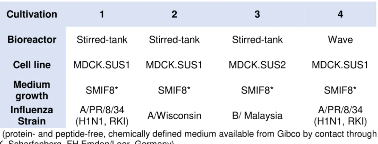
Table 1. Cultivations considered for MFA and PLS modeling

Cultivation 1 2 3 4

Bioreactor Stirred-tank Stirred-tank Stirred-tank Wave

Cell line MDCK.SUS1 MDCK.SUS1 MDCK.SUS2 MDCK.SUS1 Medium

growth SMIF8* SMIF8* SMIF8* SMIF8*

Influenza Strain

A/PR/8/34

(H1N1, RKI) A/Wisconsin B/ Malaysia

A/PR/8/34 (H1N1, RKI)

*_{(protein- and peptide-free, chemically defined medium available from Gibco by contact through}

K. Scharfenberg, FH Emden/Leer, Germany).

For each cultivation data for the biomass, substrates, products, time points and standard deviations were given. Cell numbers in suspension were determined by trypan blue dye exclusion method with ViCell XR Cell Counter from Beckman Coulter. Concentrations of glucose, lactate, glutamine, glutamate and ammonia in the supernatant were measured by Bioprofile 100 plus from IUL instruments. The concentrations of amino acids were measured using anion exchange chromatography (Dionex AAS equipment).

Treatment and Data Analysis

The first step consisted in making a functional representation of the concentration data using cubic smoothing splines.

Cubic smoothing splines are a form of interpolation where the interpolant is a piecewise polynomial called spline [27, 28]. As they are described by several

polynomials, they can make a more realistic description of the data and avoid Runge’s

phenomenon, an oscillation problem that occurs at the edges of an interval when using polynomial interpolation with polynomials with high degree [29]. For that reason, spline interpolations are preferred over polynomial interpolations.

The spline function (1) has a smoothing parameter, p, that can be chosen from the interval [0 – 1] and depending on its value it describes the data more roughly (p=0) (because the objective function for parameter identification contains the second derivative D2_𝑓as a regulation term), or it can act as a ‘natural' cubic spline interpolant

(20)

5 The objective function for parameter identification of the smoothing spline reads,

𝑝 ∑𝑛𝑗=1𝑤(𝑗)|𝐶𝑖(𝑗) − 𝑓(𝑡(𝑗))|2+ (1 − 𝑝) ∫ 𝛽(𝑥)|𝐷2𝑓(𝑥)|2 𝑑𝑥 (1)

where j = [1, …, n] is the number of points at which concentration data are available; Ci

represents the experimental data for each concentration; w is the weight of each point Ci,j, the default value for the weight is one; t represents the time of each entry j; β is the

piecewise constant weight function; D2_ƒ_{denotes the second derivative of}_ƒ_.

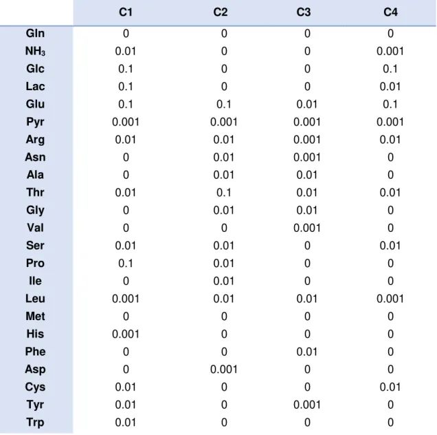
The following table contains the smoothing parameters, p, attributed to each compound for each cultivation when applying cubic smoothing splines.

Table 2. Smoothing parameters attributed for each compound present on each cultivation

Parameter estimation was made by using an algorithm (csaps; MATLAB, the Mathworks, 2013).

C1 C2 C3 C4

Gln 0 0 0 0

NH3 0.01 0 0 0.001

Glc 0.1 0 0 0.1

Lac 0.1 0 0 0.01

Glu 0.1 0.1 0.01 0.1

Pyr 0.001 0.001 0.001 0.001

Arg 0.01 0.01 0.001 0.01

Asn 0 0.01 0.001 0

Ala 0 0.01 0.01 0

Thr 0.01 0.1 0.01 0.01

Gly 0 0.01 0.01 0

Val 0 0 0.001 0

Ser 0.01 0.01 0 0.01

Pro 0.1 0.01 0 0

Ile 0 0.01 0 0

Leu 0.001 0.01 0.01 0.001

Met 0 0 0 0

His 0.001 0 0 0

Phe 0 0 0.01 0

Asp 0 0.001 0 0

Cys 0.01 0 0 0.01

Tyr 0.01 0 0.001 0

(21)

6 Figure 1 serves to explain how this ascription was made. Whenever a compound showed linear behavior the p value attributed was equal to zero, as it is demonstrated by the second and third cultivations (red and yellow). The more oscillations a compound showed the greater the p value. In the first cultivation (dark blue), lactate showed more oscillation, therefore a p value equal to 0.1 was assigned, whereas in the fourth cultivation (light blue) since the oscillation was smoother, a p value equal to 0.01 was given. Following this criteria the smoothing parameters were appointed.

When applying this type of interpolation, the concentrations of the experimental data start to depend not only from time but also from the smoothing parameter (2). As our approach is a differential one, the functions obtained for each concentration with the spline interpolation were differentiated over time (3), and using material balance equations, the extracellular rates, 𝑣(𝑡) were calculated (4 -5),

𝑐 = 𝑓(𝑡, 𝑝) (2)

𝑑𝑐 𝑑𝑡 =

𝑑𝑓(𝑡,𝑝) 𝑑𝑡 (3)

−𝑑𝑐_𝑑𝑡= 𝑣 ∗ 𝑋𝑣 (4)

−𝑑𝑐_𝑑𝑡∗_𝑋𝑣1 = −𝑑𝑓(𝑡,𝑝)_𝑑𝑡 ∗_𝑋𝑣1 = 𝑣(𝑡) (5)

where 𝑋_𝑣 is the viable cell concentration.

Note that, in the case of ammonia (6) and glutamine (7), different material balance equations had to be considered because it is known that a spontaneous

(22)

7 decomposition has influence on the formation or/and consumption of the compounds [30, 31]. The considered equations were,

( −dfammonia(t,p)_d𝑡 + 𝑘 ∗ [𝑎𝑚𝑚𝑜𝑛𝑖𝑎]) ∗_𝑋𝑣1 = 𝑣𝑎𝑚𝑚𝑜𝑛𝑖𝑎(𝑡) (6)

( −dfGln(t,p)_d𝑡 − 𝑘 ∗ [𝐺𝑙𝑛]) ∗_𝑋𝑣1 = 𝑣𝐺𝑙𝑛(𝑡) (7)

Metabolic Flux Analysis (MFA)

MFA: Calculation of the intracellular flux distributions

MFA is a constraint based mathematical method that permits to quantify intracellular fluxes if enough measured fluxes are calculated and given a metabolic network. The following assumptions are based on general MFA theory [32-35].

As mentioned before, the metabolic network used was developed by Wahl et. all [16]. The metabolic pathways considered were glycolysis, the pentose phosphate pathway, the TCA cycle, the glyoxylate shunt, cellular respiration, biosynthesis, the degradation of amino acids, the biosynthesis of biomass and an ATP consumption reaction. Two mechanisms of membrane transport were taken into account. The first between the extracellular medium and the cytoplasm and the second between the cytoplasm and the mitochondria. The biomass components considered were proteins, lipids, DNA, RNA and carbohydrates. The biomass composition was determined from experimental data and from literature [16].

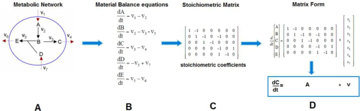
Figure 2. Schematic representation of Metabolic Flux Analysis first steps to calculate intracellular fluxes. (A) Development of a metabolic network of a certain system, (B) Formulation of the respective material balance equations for each metabolite present in the model, (C) Creation of a stoichiometric matrix based on stoichiometric coefficients, (D) Representation of the resulting data into a matrix form.

(23)

8 𝑑𝑐

𝑑𝑡= 𝐴 ∗ 𝑣 − 𝜇 ∗ 𝑐 (8)

where A is an n x m matrix of stoichiometric coefficients, v an m-dimensional flux vector, µ is the specific growth rate (h-1_{) and c is the concentration of each metabolite (µmol/L)}

(Figure 2).

It is assumed that the intracellular concentrations of the different metabolites rapidly adjust to new levels, even if a perturbation is observed in the extracellular environment by the cells, wherefore quasi-steady state can be assumed [36]. This means that there is no metabolite accumulation over time. Also the fluxes v are usually much greater than the product µ*c, wherefore the latter term can be dropped and so equation (8) turns into,

0 = 𝐴 ∗ 𝑣 (9)

The system can be separated into measured and unmeasured fluxes to, 0 = 𝐴𝑘∗ 𝑣𝑘+ 𝐴𝑢∗ 𝑣𝑢 (10)

where the first term in the right side represents the known part (which includes the measured fluxes, 𝑣_𝑘) and the second term in the right side represents the unknown part (which includes the intracellular fluxes, 𝑣_𝑢).

Since the metabolic model comprises 134 reactions and has 71 metabolites, at least 63 fluxes (degrees of freedom) needed to be measured to yield a determined system. In such case, the equation to calculate the intracellular fluxes, 𝑣_𝑢, would be,

𝑣𝑢 = − 𝐴−1𝑢 ∗ 𝐴𝑘∗ 𝑣𝑘 (11)

However, after some considerations, 21 fluxes were set to zero based on assumptions made by Sidorenko et al. [13], another 11 fluxes were set to zero based on the metabolism of amino acids and because no data regarding virus production was considered, other 14 fluxes were set to zero. Additionally, 24 extracellular fluxes were calculated from the experimental data. So in total 70 fluxes, 𝑣_𝑘, were considered.

As described by Klamt et al [37], the system can then be classified based on the number of measured fluxes in terms of determinacy and redundancy,

 Undetermined if rank(𝐴_𝑢) < number of 𝑣_𝑢, where there are not enough linearly independent constraints for computing all rates of 𝑣_𝑢 uniquely;

 Determined if rank(𝐴_𝑢) ≥ number of 𝑣_𝑢, where there are enough linearly independent constraints for computing all rates of 𝑣_𝑢 uniquely;

 Redundant if rank(𝐴_𝑢) < m;

 Not redundant if rank(𝐴_𝑢) = m, with m equal to the number of metabolites present in the metabolic network.

In this case, as there are more measured fluxes than degrees of freedom, and consequently there are more equations available than the minimum needed for determinations of the unknown fluxes the system can be classified as determined and redundant and instead of using equation (11), Moore-Penrose pseudo-inverse matrix was used to solve the system,

(24)

9

MFA: Data accuracy

After the unknown fluxes were calculated, the accuracy of both known and unknown fluxes was checked using redundant measurements, R. If the system assumed that the biochemistry behind the metabolic model was correct and there were no errors in the measurements one should verify,

0 = 𝑅 ∗ 𝑣𝑘 (13) where,

𝑅 = 𝐴𝑘− 𝐴𝑢∗ 𝐴𝑢#∗ 𝐴𝑘 (14)

However, it is most common that experimental data sets present noise or/and in some cases, systematic errors. So equation (13) can be transformed to,

𝑒 = 𝑅𝑟𝑒𝑑∗ 𝑣𝑘 (15)

where 𝑅_𝑟𝑒𝑑 is the reduced redundancy matrix containing only the independent rows of R. With this equation one could then analyze the magnitude of the errors of the data set.

MFA: Data consistency

To evaluate the consistency of the data and model, the consistency index, h (16) was calculated,

ℎ = 𝑒𝑇_{∗ 𝑌}−1_{∗ e}₍₁₆₎ where,

𝑌 = 𝑅𝑟𝑒𝑑∗ 𝑌𝑏∗ 𝑅𝑟𝑒𝑑𝑇 (17)

For that, Monte Carlo method was applied to generate 1000 data matrices based on the standard deviations of the experimental data. This procedure gave an approximation of the correct variance-covariance matrix, 𝑌_𝑏 which was assumed to be diagonal meaning that the measurements are uncorrelated. Monte Carlo simulations are important tools when it comes to estimate model parameters and to perform sensitivity analysis [38].

It is known that when the measurements are uncorrelated, the consistency index is χ2 _{distributed [26].}

The comparison between h and the χ2_{test function provides an idea of how}

consistent is the experimental data with the assumed biochemistry. For this, reduced redundancy measurements were used as the degrees of freedom for statistical hypothesis testing at a 95% confidence level.

Consistent results should obey this condition h < χ2_{. If at a high confidence level}

one obtains a consistency index greater than the value of the χ2 _{distribution, than there}

(25)

10

MFA: Data reconciliation

Finally, to obtain a better estimation for both known and unknown fluxes, Weighted Least Squares (WLS) method was applied according to the following equations,

𝑣𝑘,𝑐𝑜𝑟𝑟 = (𝐼 − 𝑌𝑏∗ 𝑅𝑟𝑒𝑑∗ (𝑅 ∗ 𝑌𝑏∗ 𝑅𝑟𝑒𝑑)−1∗ 𝑅) ∗ 𝑣𝑘 (18)

𝑣𝑢,𝑐𝑜𝑟𝑟 = −𝐴#𝑢∗ 𝐴𝑘∗ 𝑣𝑘,𝑐𝑜𝑟𝑟 (19) where I is the identity matrix.

Partial Least Squares (PLS)

PLS: Overview

With both extracellular concentrations and cell’s fluxome calculated with material

balance equations and MFA, respectively, the PLS method was applied to verify how these two variables relate with each other and also to determine the optimal concentrations to reach a high biomass growth rate for both a batch and a continuous system.

PLS is a statistical regression technique highly suited for analyzing high-dimensional data [39].

It differs from conventional regression methods because besides being able to analyze data with many noise, it can efficiently examine the structural relationship between independent variables, X, and dependent variables, Y even when there are more variables in X than (independent) observations [40-43]. This feature is of most interest since the goal of this work is to understand the impact of the medium concentrations (independent variables) on the flux distribution (dependent variables).

Usually, the dependent variables are difficult to obtain or because the techniques used are time-consuming or because they are expensive, whereas independent variables are easy and cheap to obtain [39].

PLS has the particularity of making a regression model so that in the future only independent variables are needed to predict the dependent variables, turning this method into a valuable tool.

(26)

11

PLS: Pretreatment and Cross Validation

Before doing any type of regression analysis and because data sets differ in range and size, a pretreatment of the data was made. This is usually performed by scaling the data. That way each variable can have the same weight when there is an absence of knowledge about the relative importance of the variables. This scaling consists in center each variable by subtracting their averages and by dividing them by its standard deviation, the so called, auto-scaling [41, 49].

The accuracy of the predictions depend on the number of latent variables. This number tells us how good the model is in a way that it consistently precisely predicts the intracellular flux distribution, Y, with new medium concentrations, X. If one uses a low number of LV, information can be lost, but since data is never noise free, some variables will only add noise, so a high number of LV is also not desirable [50]. In order to create a valid PLS model with optimal prediction power, a cross validation technique was applied to determine the optimal number of latent variables [41, 42].

In this case, single cross validation technique was applied. With this technique, part of the data, in this case 1/3 of it, was removed from both independent set and dependent set and used as validation set. The remainder that forms the training set was used to develop several training models in which each model was based on one LV. In order to identify which LV gave a better prediction power, one to many LV were tested, so for instance the first training model was based on 1LV, the second was based in 2LV and so on and so forth. For each of the training model, a prediction of the validation set was made and the respecting modelling errors were calculated. These errors were calculated based on the difference between the actual values of the validation set (measured values) and the values predicted by the training model (observed values). The sum of squares of the errors was then calculated as the sum of squares of all squared errors. The model with the lowest error was selected as the best and, consequently the number of LV [50, 51].

(27)

12

PLS: PLS model

The PLS model was built using the complete data set for both Y and X and the number of LV estimated with the cross validation technique. With the algorithm npls (Copyright (C) 1995-2006 Rasmus Bro & Claus Andersson; Copenhagen University, DK-1958 Frederiksberg, Denmark, rb@life.ku.dk) the best model parameters values i.e., scores, loadings and the regression coefficient matrix were calculated. With such parameters and with the algorithm npred (Copyright (C) 1995-2006 Rasmus Bro & Claus Andersson; Copenhagen University, DK-1958 Frederiksberg, Denmark, rb@life.ku.dk), new input sets were used to make flux predictions.

With the PLS model established, it was finally possible to evaluate the impact of the medium concentration into each flux distribution and to elaborate strategies for the optimizations proposed.

PLS: Optimization for a continuous system

Figure 4. After the selection of the inputs through the PLS model, new predictions were made. Being the biomass growth rate, the rate of interest a mathematical maximization function, fmincon (MATLAB, the Mathworks, 2013) was applied in order to determine the optimal medium concentrations that resulted in a maximization of the biomass growth rate.

When performing a continuous operational mode, fresh medium is constantly added and spent medium is collected so the extracellular environment is inalterable over time [18]. This means that given a specific set of inputs or concentrations the intracellular rates will also be constant including the biomass growth rate. Therefore, optimal concentrations that would result in a maximum biomass growth rate would lead to high cell densities.

Using the PLS model, several sets of medium concentrations based on the experimental data were used as inputs and new predictions were made. The selection of the input was made by evaluating which one had the best prediction of the biomass growth rate.

(28)

13

PLS: Optimization for a Batch system

In this case, since the extracellular concentrations change over time the intracellular fluxes also change so a different approach had to be considered. In this case, the goal is to maximize the biomass concentration at the end of the batch, tf (Figure 5). Again the set of concentrations was selected based on the performance it had on the biomass growth rate. A time range and an additional value corresponding to the initial biomass had also to be considered. New fluxes were predicted by the PLS model and by multiplying their value with the initial biomass the derivatives of the concentrations were calculated. Next, with solver function (ode45; MATLAB, the Mathworks, 2013) integration of the derivatives was made in order to calculate the concentration values over time. Finally, the maximization function was used once again to determine the optimal concentrations that contributed to a maximum value of the biomass concentration.

(29)

14

Results and discussion

In this work, the impact of the medium concentrations on the flux distribution is studied and an optimization strategy is proposed in order to reach high cell densities for both a batch and a continuous system.

For that, calculation of the cell fluxome is made using classical metabolic flux analysis, which is then linked to the extracellular environment using a PLS model.

Since MFA is based on the quasi steady-state assumption, the intracellular metabolite concentrations should be constant over time (see Materials and Methods). That said, the time range considered was comprehended from moments after the exponential phase had begun until moments before the infection had been made. During this interval, it is expected that the quasi steady-state assumption holds (example in Figure 6).

Figure 6. Concentration profile of Lactate excretion over time for Cultivation 1. Solid lines represent the time range defined.

Spline interpolation

Figure 7. First steps applied in the medium concentrations in order to calculate the extracellular fluxes.

(30)

15 the time and by applying material balance equations the extracellular flux values were calculated (Figure 7).

Before estimating the intracellular fluxes with MFA, a detailed analysis of the cell metabolism was made based on the evaluation of each medium concentration, in order to see whether the cell was behaving as expected or not.

MDCK Metabolism

Because the same cell line and medium (SMIF8) were used in all cultivations, a similar behavior in terms of metabolism was expected. (Note that the cell line used in C3, MDCK.SUS2, derives from the cell line used in the other cultivations).

However, since the cultivations were not performed at the same time, and since the medium composition changes along the time, the initial concentrations were not the same resulting into a different metabolism by the cell in each cultivation, i.e. different flux distributions.

Moreover, C4 was operated in a distinct operational system, namely a wave reactor, which according to Lohr et al also influences the cell metabolism [15].

Carbon source metabolism

The primary carbon sources for ATP production are glucose and glutamine. They are also responsible for the production of waste products. According to the literature, the metabolism of these two components leads to the production of ammonia and lactate, components known to inhibit the cell growth. Ammonia results from the metabolism of amino acids, mainly from glutamine degradation, and lactate is synthesized from the conversion of glucose to pyruvate during the glycolytic pathway [52]. Figure 8 and figure 9 demonstrate the metabolism of these compounds.

(31)

16 Looking at the representations, it seems that most of the glucose up taken by the cell is transformed to lactate, as expected. Comparing all cultivations, C1, presents the highest lactate concentration compared to the other cultivations.

Figure 9. Concentration values for ammonia release and glutamine uptake during the exponential phase of MDCK suspension cells with respective standard deviations. (A) Represents the first cultivation; (B) represents the second cultivation; (C) represents the third cultivation; (D) represents the fourth cultivation; gln ( ), NH3 ( ).

In the case of glutamine consumption and ammonia excretion, results also seem to be in accordance to what is expected, as most of the glutamine is converted to ammonia. Starting concentrations of glutamine are close to 6000 µmol which according to V. Lohr et. al. [15] the risk of reaching inhibiting ammonia concentrations is high. Again, C1 presents the highest ammonia concentration compared to the other cultivations. C1 had the higher initial concentration of glucose (20780.97 µmol/L) when compared to the other cultivations (18134.54 µmol/L for C2; 18315.47 µmol/L for C3; and 17868.49 µmol/L for C4) so a higher concentration of lactate was expected, however C4 had the higher initial concentration of glutamine (5600.94 µmol/L) when compared to the other cultivations (4672.29 µmol/L for C1; 5320.69 µmol/L for C2; and 5417.59 µmol/L for C3) so higher concentrations of ammonia were expected for this cultivation. It might be that, in C1 other pathways than the usual are contributing for the production of ammonia leading to such high values.

(32)

17 Pyruvate is an intermediate of lactate production [11], so a decrease over time is expected as it is shown in Figure 10. Data not shown for C3 as not enough measurements were made.

Metabolism of essential and non-essential amino acids

Essential amino acids (e.g., histidine, isoleucine, leucine, methionine, phenylalanine, threonine, tryptophan and valine) were consumed by the cell in all cultivations, as expected. In contrast to the essential amino acids, part of the non-essential amino acids were consumed whilst others were released. Arginine, cysteine, tyrosine and aspartate concentrations showed a decrease over time, while alanine and glycine concentrations increased. Asparagine concentration was almost constant during the considered time. Glutamate concentration showed not only a decrease over time but also several oscillations, which might affect the calculation of both extracellular and intracellular fluxes. Due to problems in the experimental data from proline and serine measurements could not by analyzed. For a better understanding see Annex 1.

Biomass synthesis

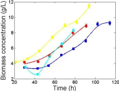
Since our goal is to understand how the extracellular environment affects the cell regulation (i.e., flux distribution) in order to reach high cell densities, both viable biomass concentration and biomass growth rate were evaluated during the exponential phase to be compared with the future results (Figure 11).

Figure 11. Biomass concentration during the exponential phase of MDCK suspension cells for all cultivations. The solid lines represent the model fit. Cultivation 1 is represented in dark blue and has a final cell density of 9.24 g/L; Cultivation 2 is represented in red and has a final cell density of 8.88 g/L; Cultivation 3 is represented in yellow and has a final cell density of 11.50 g/L; Cultivation 4 is represented by light blue and has a final cell density of 8.28 g/L.

Biomass growth rates were calculated with a linear regression model (data not shown). The first three cultivations resulted in similar growth rates ≈ 0.014 h-1_{, which}

(33)

18 biomass growth rate (0.022 h-1_{) resulting in a duplication time of 31 hours and 51}

minutes.

Table 3. Final cell density (g/L), biomass growth rate (h-1) and duplication time (h) for all cultivations during the exponential phase.

C1 C2 C3 C4

Duration of the

exponential phase (h) 84.5 61.25 73.24 47.5

Final cell density (g/L) 9.24 8.88 11.50 8.28

Biomass growth rate

(𝒉−𝟏) 0.014 0.014 0.014 0.022

Duplication Time 49h 51 min 49h 51 min 49h 51 min 31h 51 min

Observing Table 3, a few considerations can be outlined. Since C1 has the longest exponential phase, higher biomass concentrations were expected. However, C3, which shows the second longest phase, presents higher values. As told before, more lactate and ammonia were produced in C1 so there might be occurring some inhibition affecting the cell growth, even though both cultivations show the same biomass growth rate [53, 54].

C4 has almost half of the duration of C1 and yet their final cell density is similar. This can be explained by the fact that C4 has a higher biomass growth rate and also because C4 is operated in a wave bioreactor. These types of operational systems have already proven to reach higher cell densities and lower duplication times when compared to stirred-tank bioreactors [15].

Metabolic Flux Analysis

(34)

19 As mentioned before, MFA is a constraint based-model that permits the calculation of the flux distribution (see Materials and Methods). At this point, the extracellular fluxes were estimated from the medium concentrations using spline approximations and material balance equations. Also, a metabolic network had already been selected and the constraints defined (Figure 12).

Extracellular flux distribution

Firstly an analysis of the extracellular fluxes was made. A positive signal means that the reactions are carried in the direction of the arrow and the negative signal means that the reactions are carried out in the opposite direction of the arrow.

Highest flux values are registered for glucose and lactate. Since glucose is the main source of ATP and because the cell does not function without it, a high rate for the consumption of this compound is expected and since lactate is the resulting product from the consumption of glucose, a high lactate rate is also expectable.

Regarding the other elements, most of them seem to have similar rates. C4 presents high flux values for most of the compounds, meaning that in this case, the cell metabolism should be more active, which, as seen before, is expected since this cultivation is operated in a wave bioreactor.

The direction of the fluxes also seem to be in accordance with the literature, except for glutamate which appears to be in the opposite direction. As seen in the Materials and Methods section, one of the MFA constraints is the quasi steady-state assumption, which signifies that the metabolite concentrations should be constant over time. As mentioned before, glutamate shows several oscillations which might be affecting the calculation of the fluxes.

Table 4. Average extracellular fluxes (µmol/cell/h) and respective standard deviations calculated using a Monte Carlo approach during the time range considered for each cultivation.

Reaction C1 C2 C3 C4

Gln 0.33 ATP_c ==>

GLN_c 3.04 ± 1.10 1.29 ± 2.06 2.49 ± 1.26 5.82 ± 3.68

NH3 <==> NH3_c -4.06 ± 1.69 -2.98 ± 0.45 -4.05 ± 0.36 -4.81 ± 1.14

Glc Glc → Glc_c 12.20 ± 9.08 10.82 ± 1.40 13.54 ± 0.96 15.28 ± 10.77

Lac <==> Lac_c -29.61 ± 6.92 -16.63 ± 1.12 -24.38 ± 0.85 -21.53 ± 5.82

Glu ATP_c ==>

GLU_c -1.33 ± 0.35 -0.54 ± 0.31 -0.32 ± 0.18 -2.07 ± 0.48

Pyr 0.33 ATP_c ==>

Pyr_c 2.17 ± 0.07 2.41 ± 0.08 0.00 ± 0.00 3.14 ± 0.11

Arg 0.33 ATP_c ==>

ARG_c 0.36 ± 0.34 0.61 ± 0.31 0.54 ± 0.18 0.80 ± 0.49

Asn 0.33 ATP_c ==>

ASN_c 0.01 ± 0.25 0.46 ± 1.04 0.18 ± 0.63 0.71 ± 0.65

Ala ALA_c ==> 2.37 ± 0.21 2.71 ± 1.12 5.66 ± 1.91 2.77 ± 0.48

Thr 0.33 ATP_c ==>

(35)

20

Gly GLY_c ==> 0.36 ± 0.13 0.14 ± 0.44 0.34 ± 0.61 0.02 ± 0.24

Val 0.33 ATP_c ==>

VAL_c 0.55 ± 0.07 0.37 ± 0.09 0.53 ± 0.21 0.96 ± 0.16

Ile 0.33 ATP_c ==>

ILE_c 1.06 ± 0.22 1.16 ± 0.79 1.00 ± 0.19 2.00 ± 0.52

Leu 0.33 ATP_c ==>

LEU_c 0.98 ± 0.22 1.30 ± 0.28 1.05 ± 0.31 2.29 ± 0.27

Met 0.33 ATP_c ==>

MET_c 0.15 ± 0.09 0.15 ± 0.12 0.17 ± 0.08 0.42 ± 0.19

His 0.33 ATP_c ==>

HIS_c 0.12 ± 0.10 0.10 ± 0.04 0.13 ± 0.03 0.26 ± 0.08

Phe 0.33 ATP_c ==>

PHE_c 0.13 ± 0.07 0.22 ± 0.10 0.04 ± 0.38 0.40 ± 0.16

Asp ATP_c ==>

ASP_c 1.88 ± 0.00 2.69 ± 0.00 3.78 ± 0.00 4.07 ± 0.00

Cys 0.33 ATP_c ==>

CYS_c 0.06 ± 1.62 0.08 ± 2.33 0.09 ± 1.69 0.21 ± 4.17

Tyr 0.33 ATP_c ==>

TYR_c 0.10 ± 0.09 0.10 ± 0.02 0.14 ± 0.01 0.33 ± 0.11

Trp 0.33 ATP_c ==>

TRP_c 0.04 ± 0.13 0.03 ± 0.03 0.05 ± 0.06 0.09 ± 0.05

Intracellular flux distribution

Secondly, the MFA model performed the estimation of the intracellular fluxes. Here, a detailed analysis was made (Table 5).

Table 5. Average intracellular fluxes estimated by MFA (µmol/cell/h) during the time range considered for each cultivation.

No. Reaction C1 C2 C3 C4

Glycolysis

66 Glc_c ==> G-6P_c 12.20 10.82 13.54 15.28

2 G-6P_c <==> F-6P_c 13.73 6.21 11.49 7.61

3 F-6P_c <==> GAP_c 12.27 4.23 9.59 5.00

55 GAP_c <==> PGA_c 22.61 5.87 16.68 6.57

56 PGA_c <==> PEP_c 22.61 5.87 16.68 6.57

57 PEP_c ==> Pyr_c 45.19 22.26 29.79 30.70

Pentose Phosphate Pathway (PPP)

60 R-5P_c <==> F-6P_c + GAP_c -0.73 -0.99 -0.95 -1.31 61 R-5P_c <==> GAP_c + S-7P_c -0.73 -0.99 -0.95 -1.31 62 GAP_c + S-7P_c <==> F-6P_c -0.73 -0.99 -0.95 -1.31

Anaplerotic Reactions

5 Pyr_m ==> A-CoA_m -1.18 -1.57 -1.52 -1.77

6 Mal_m <==> Pyr_m -23.07 -13.39 -6.27 -21.54

68 Mal_c <==> Pyr_c 8.90 12.04 11.57 15.84

(36)

21 TCA cycle

7 A-CoA_m + OAA_m ==> Cit_m 7.56 8.92 8.40 11.12

71 Cit_m <==> a-Ket_m 0.54 -0.55 -0.73 -1.40

10 a-Ket_m ==> S-CoA_m 1.51 6.30 8.43 8.14

104 S-CoA_m <==> Fum_m 8.73 13.87 16.12 16.67

9 Fum_m <==> Mal_m 8.73 13.87 16.12 16.67

8 Mal_m <==> OAA_m 7.56 8.92 8.40 11.12

72 Mal_c <==> OAA_c 16.91 8.41 4.44 14.03

74 Cit_c ==> OAA_c + A-CoA_c 7.02 9.48 9.13 12.53

Amino acid degradation

11 GLU_m <==> a-Ket_m 7.16 12.44 13.18 13.66

12 GLN_c <==> GLU_c 1.24 -1.77 -0.18 0.47

16 ALA_c <==> Pyr_c -3.45 -4.63 -7.46 -6.04

18 ASP_c <==> OAA_c -1.35 -1.50 -0.46 -2.42

42 ARG_c <==> GLU_c 2.00 1.78 2.14 0.91

43 ASN_c <==> ASP_c -0.43 -0.25 -0.54 -1.05

45 ILE_c ==> S-CoA_m + A-CoA_m 2.99 3.56 3.33 4.54

46 LEU_c ==> A-CoA_m 1.38 1.58 1.51 1.86

48 MET_c ==> S-CoA_m 1.02 0.63 1.01 0.12

50 PRO_c <==> GLU_c -7.32 -1.33 -1.10 -1.56

51 THR_c ==> Pyr_c 1.03 0.92 1.11 0.11

52 TRP_c ==> A-CoA_m 0.80 1.10 1.04 1.39

53 VAL_c ==> S-CoA_m 3.21 3.38 3.34 3.88

77 GLY_m <==> SER_m -3.00 -4.12 -4.05 -6.02

78 SER_c <==> Pyr_c -3.74 -5.96 -7.51 -3.85

80 CYS_c ==> Pyr_c 1.41 1.42 1.63 1.42

Other reactions

13 Pyr_c <==> Lac_c 29.61 16.63 24.38 21.53

79 NADH_m <==> NADPH_m 15.92 0.96 -6.90 7.88

Lipid Biosynthesis

87 CH 0.18 0.24 0.23 0.32

88 PC 0.68 0.92 0.88 1.21

89 PE 0.26 0.35 0.33 0.46

90 PS 0.03 0.03 0.03 0.05

91 PG 0.07 0.09 0.09 0.12

92 PI 0.09 0.13 0.12 0.17

93 SM 0.08 0.11 0.11 0.15

Respiration reactions

75 FADH2_m ==> ATP_m 18.22 24.51 26.54 28.58

(37)

22 Membrane Transport (c – m)

58 Pyr_c <==> Pyr_m 20.87 10.91 3.64 19.67

73 Mal_c + Cit_m <==> Mal_m + Cit_c 7.02 9.48 9.13 12.53

59 a-Ket_m <==> a-ket_c 6.18 5.59 4.02 4.12

86 Mal_m <==> Mal_c 31.27 27.82 23.12 39.62

76 ATP_m <==> ATP_c 35.92 98.48 127.62 94.57

82 GLU_c <==> GLU_m 7.16 12.44 13.18 13.66

103 SER_c <==> SER_m 3.00 4.12 4.05 6.02

102 GLY_c <==> GLY_m -6.00 -8.23 -8.10 -12.05

84 NH3_c <==> NH3_m -4.16 -8.32 -9.13 -7.64

70 CO2_c <==> CO2_m 22.58 10.24 0.97 19.73

Membrane transport (m – c)

22 <==> CO2_c -11.87 -20.53 -26.42 -21.90

25 ==> O2_c 15.58 29.86 35.60 31.04

64 ATP_c ==> 13.26 9.57 63.87 -77.66

81 Urea_c <==> 2.00 1.78 2.14 0.91

Observing the flux values related to glycolysis, it seems that glucose is effectively converted to pyruvate (reaction 57). Pyruvate can then be carried from the cytoplasm to the mitochondria and undergo to anaplerotic reactions or it can be converted to lactate. Although there is some pyruvate being transported to the mitochondria (reaction 58), most of it is converted to lactate as indicated by the highest fluxes (reaction 13). Concerning PPP, flux values were low and stayed constant along the reactions (reactions 60 to 62).

The anaplerotic reactions are partly active. More activity is observed for the cytosolic reactions (reaction 68 and 69). As seen before, part of the pyruvate formed in the cytoplasm is transported to the mitochondria (reaction 58) and then converted to malate (reaction 6). Malate is transported to the cytoplasm (reaction 86) and metabolized again to pyruvate (reaction (68) and to oxaloacetate (reaction 72). Curiously the reaction carried out by pyruvate dehydrogenase operates in the opposite direction (reaction 5), demonstrating some inconsistency thought the magnitude of these flux values is relatively low in relation to other pyruvate fluxes. Since this occurs, no acetyl-CoA is produced.

Despite acetyl-CoA is not being produced during anaplerotic reactions, some activity is detected in the TCA cycle. In this case, the main precursors of this compound are isoleucine, leucine and tryptophan (reaction 45, 46 and 52).

Concerning the amino acid degradation and lipid biosynthesis, similar fluxes are observed for every cultivation, except for the reaction responsible for the production of glutamate from glutamine (reaction 12). In this case, only in C1 and C4 glutamine is converted to glutamate and C1 presents the highest conversion rate, meaning that this might be the pathway contributing for the high levels of ammonia as the latter compound is released in this reaction.

(38)

23 The highest flux values are observed for ATP reactions (reaction 64 and 76).

Looking carefully, arginine degradation (reaction 42) seems to be responsible for the synthesis of urea (reaction 81).

Overall the cell is behaving as expected in all cultivations and not much discrepancies are observed when comparing the fluxes. Even though the consumption of glucose is similar for all cultivations, a much higher excretion of lactate is observed for C1 due to high conversion rates of pyruvate. In this case, there might be some other pathways contributing for the high conversion rate and because of that, more waste product is excreted affecting the biomass growth. As expected, due to a high extracellular activity, cultivation 4 shows, in most of the cases, a high intracellular activity when comparing with the other cultivations.

Consistency Index

In order to validate the MFA model, a consistency test was made, i.e. the consistency index (h value) was calculated along the cultivations, (Figure 13). It can be seen that all cultivations present an h value lower than the corresponding χ2_value,

meaning that the assumed biochemistry behind the metabolic network is consistent with the measured extracellular fluxes, validating the model (see Materials and Methods).

Figure 13. Consistency index (h) over time for each cultivation with test function (χ2 (0.95, 8) = 15.50). (A) Cultivation 1; (B) Cultivation 2; (C) Cultivation 3; (D) Cultivation 4.

Overview of the flux distribution

To get an impression of the flux distribution for each cultivation, a 3-D analysis was made (Figure 14).

(39)

24

Figure 14. Metabolic flux distribution for all cultivations. (A) Cultivation 1; (B) Cultivation 2; (C) Cultivation 3; (D) Cultivation 4.

Partial Least Squares

Depending on the environment the cell will behave in a specific way, with a characteristic phenotypic trait, expressed as a result of the intracellular flux distribution.

(40)

25

Number of latent variables

The first step in order to create a PLS model, was to determine the number of latent variables that would best decompose both sets of variables and, consequently result in a model with best predictive power. This was possible using cross validation techniques.

Cross validation is often used to validate a model. There are several cross validation techniques that can be used to serve this purpose. In this case, single cross validation technique was applied as seen in the Materials and Methods section.

The principal behind this technique is that the optimal number of LV corresponds to the minimum modelling error obtained for the estimation of the validation set.

Figure 15 shows the plot of the modelling error against the number of LV for the validation set when applying this technique. In this case, the minimum error found for the validation set corresponds to a number of LV equal to 11.

Figure 15. Modelling error obtained for each LV with single cross validation technique for the validation set.

What was seen is that as the number of LV increases, the error of the validation set also increases (data not shown). This means that with a high number of LV the predictions would only get worse as probably only noise or irrelevant data was being included in the model, affecting the predictions. Herein, the goal was to obtain a model based on the number of LV that could include all relevant data and at the same time minimize redundant data.

(41)

26

Table 6. Training model decomposition results in terms of % of explained variance over number of latent variables.

Latent Variables Variance X (%) Variance Y (%)

1 57.98 10.22

2 79.34 18.54

3 86.54 25.62

4 90.47 35.90

5 93.75 45.03

6 95.35 53.76

7 98.47 57.28

8 99.01 62.78

9 99.18 67.78

10 99.49 69.41

11 99.61 73.68

PLS model

Having identified the number of LV, the PLS model was built. In this case the resulted model explained almost 70% of the variance in Y (Table 7).

Table 7. PLS model decomposition results in terms of % of explained variance over number of latent variables.

Latent Variables Variance X (%) Variance Y (%)

1 49.31 6.60

2 74.07 12.42

3 83.72 21.41

4 87.58 34.07

5 92.03 43.85

6 95.21 47.91

7 97.69 51.86

8 98.27 58.01

9 98.69 60.93

10 99.17 65.20

11 99.39 67.77

(42)

27 by the observation that the greatest deviations seem to have a cyclic behavior, which is an artifact coming from greater or lower measured concentration value.

Figure 16. Correlation between predicted fluxes and measured fluxes.

Also very important is to analyze the model’s specific biomass growth predictions. Although the model is capable to describe the general trend of biomass growth fairly well (Figure 17), it is not very precisely describing biomass growth. One cannot forget that our model can only explain almost 70% of the Y data.

Figure 17. Prediction of the specific biomass growth rate (µ). Solid blue line represents the measured flux and solid black line represents the predicted flux.

The metabolic state of each cell, as the name implies has to do with the type of metabolism which the cell performs face to the conditions it finds. These conditions can range from the composition of the medium, the concentration of each component present in the medium to the cell's own needs.

(43)

28 It is clear that when a 3-dimensional plot is made, additional information is considered and different results are obtained when compared to a 2-dimensional plot. In both cases, the cultivation that stands out is cultivation 3 (Figure 18). In the 2-dimensional plot, while C1, C2 and C4 are close together, C3 stays more distant. On the other hand, on the 3-dimensional plot while C1, C2 and C4 present some oscillations, C3 has a more linear behavior. This means that C3 is in a different metabolic state which might be an influence of the medium composition since this cultivation has the same operating system as C1 and C2. The only thing different is the cell line that it is used, which as said before, should lead to no differences in terms of metabolism, since it derives from the cell line used in C1 and C2. Yet, as no pyruvate was considered for this cultivation (due to absence of measurements) it might be possible that the PLS model considers this cultivation to be in a distinct metabolic state. Not only pyruvate is known to be the intermediate of lactate production but it also has a huge role in the anaplerotic reactions which then affect all the other metabolic pathways such as the TCA cycle. Also, a much higher flux of the production of alanine was observed for this cultivation (Table 4).

This indicates that the PLS model can clearly identify that differences in the medium culture affect the intracellular flux distribution, in this case translated by differences in metabolic states.

Figure 18. 2D score plot and 3D score plot from the PLS model. Cultivation 1 is represented in dark blue; Cultivation 2 is represented in red; Cultivation 3 is represented in yellow and; Cultivation 4 is represented in light blue.

To evaluate the impact of each component on each flux distribution, more precisely on the biomass growth rate, elasticities were evaluated in a form of a matrix map for each cultivation in the beginning and in the final time points considered (Figure 19 and Figure 20). The elasticities present sensitivities of the fluxes with respect to each component present in the extracellular medium and therefore with their concentrations. They are obtained by multiplying both loading sets (dependent and independent) with the regression coefficient matrix of the PLS model.