Todos os direitos reservados.
É proibida a reprodução parcial ou integral do conteúdo
deste documento por qualquer meio de distribuição, digital ou
impresso, sem a expressa autorização do
REAP ou de seu autor.
Time-dependent or state-dependent pricing?
Evidence from a large devaluation episode
Celio Feltrin Jr
Bernardo Guimaraes
TIME-DEPENDENT OR STATE-DEPENDENT PRICING?
EVIDENCE FROM A LARGE DEVALUATION EPISODE
Celio Feltrin Jr
Bernardo Guimaraes
Celio Feltrin
Escola de Economia de São Paulo Fundação Getúlio Vargas (EESP/FGV) Rua Itapeva, nº 474
01332-000 - São Paulo, SP - Brasil
Bernardo Guimarães
Escola de Economia de São Paulo Fundação Getúlio Vargas (EESP/FGV) Rua Itapeva, nº 474
01332-000 - São Paulo, SP - Brasil
Time-dependent or state-dependent pricing? Evidence from a large
devaluation episode
∗Celio Feltrin Jr† Bernardo Guimaraes‡
June 2014
Abstract
State-dependent and time-dependent price setting models yield distinct implications for how frequency and magnitude of price changes react to shocks. This note studies pricing behavior in Brazil following the large devaluation of the BrazilianReal in 1999 to distinguish between models. The results are consistent with state-dependent pricing.
Keywords: state-dependent pricing, time-dependent pricing, currency devaluation, frequency of price changes.
Jel Classification: E31, E32.
1
Introduction
Are patterns of price adjustment best captured by time-dependent or state-dependent models of price setting? The answer to this question has important implications for the real effects of monetary policy. This paper explores the distinct predictions of price-setting models on how the frequency and magnitude of price adjustment react to shocks in order to distinguish between models.
In order to understand the implications of time-dependent and state-dependent price setting, consider a positive shock to the desired prices of goods (the prices that would be charged in the absence of frictions). In the simplest state-dependent models (e.g., Caplin and Spulber (1987)), a firm raises the price of its good whenever the difference between the desired and current price hits a constant threshold. Hence a positive shock to desired prices raises the frequency of price changes but the magnitude of price changes is not affected. In recent models of state-dependent price setting, shocks might have some effect on the magnitude of price changes, but the response of the frequency of price adjustment to shocks is the key feature of these models.1
∗We thank Cristine Pinto, Mauro Rodrigues Jr, Vladimir Teles and seminar participants at the Sao Paulo School of Economics
– FGV for helpful comments. We also thank IBRE-FGV and, especially, Solange Gouvea for the data. Celio Feltrin Jr gratefully acknowledges financial support from CAPES. Bernardo Guimaraes gratefully acknowledges financial support from CNPq.
†Sao Paulo School of Economics – FGV. ‡Sao Paulo School of Economics – FGV.
1
Models with time-dependent pricing yield the opposite prediction. In models that follow Calvo (1983), the frequency of price changes is exogenously given. In models with endogenous time-dependent pricing (e.g., Bonomo and Carvalho (2004)), firms optimally choose the time of the next price change when they adjust prices. In both cases, a shock that raises desired prices will not affect how long it will take for the next price change, but will raise the magnitude of the price increase when it happens.2
The Brazilian devaluation of 1999 allows us to distinguish between time-dependent and state-dependent models. Until January 1999, Brazil had a pegged exchange rate regime. The peg was then abandoned and between January 13th and February 1st, the price of 1 dollar increased from 1.2 to around 2 Reais. This very large change resulted from incremental currency depreciations in the second half of January.3
Firms in the tradable sector thus experienced a sequence of shocks to their desired prices in this period. In a world with state-dependent pricing, we would observe a large increase in the frequency of price changes for these firms. In contrast, in a world with time-dependent pricing, the frequency of price changes would not react to these shocks, but the magnitude of price changes would be affected. Non-tradable goods (services) can be used as a control group.
Using a large data set on consumer prices in Brazil from 1998 and 1999, we estimate patterns of pricing behavior for different groups of items. In the group of tradable goods, the probability of a price change dramatically increases in the second half of January. In contrast, there is no observable change in the magnitude of a devaluation. No significant effect is observed in the group of non-tradable goods. The results thus corroborate the strong predictions of state-dependent models.
This paper complements previous empirical work on this topic. Klenow and Kryvtsov (2008) contrast the implications of different models to the data on hazard rates and sizes of price changes. Gagnon (2009) shows that when inflation is above a certain threshold, higher inflation corresponds to shorter price spells. Midrigan (2010) notes that in models with state-dependent pricing, firms are more likely to change prices if idiosyncratic and aggregate shocks are positively correlated, and explores the sectoral variation in the correlation between idiosyncratic and aggregate shocks. Guimaraes, Mazini and Mendon¸ca (2014) study how the frequency and magnitude of price adjustments react to inflation shocks, but their identifica-tion relies of differences between expected and observed inflaidentifica-tion. The main distinguishing feature of this paper is the use of a large shock to desired prices of a group of goods, which allows for a clean identification and enables us to distinguish between state-dependent and endogenous time-dependent models. One caveat is that it is not clear whether the patterns
2
A simple correlation between inflation and frequency of price adjustment is not enough to test these predictions. Models of state-dependent pricing imply a positive correlation between inflation and frequency of adjustment, but so do models with endogenous time-dependent pricing. Hence a large shock is needed for this prediction to be explored.
3
While the results are specific to the Brazilian case, the test proposed in this paper could be applied to other countries that have experienced large currency devaluations in the last decades.
of price adjustment in scenarios of large devaluations can be generalized to normal times. The structure of this paper is the following. Section 2 describes the data, Section 3 presents the methodology and Section 4 presents the results.
2
Data
We use data collected by IBRE-FGV to compute the consumer price index.4 Products are
divided in seven major expenditure classes (food, housing, clothing, health and personal care, education, reading and Recreation, transport and miscellaneous expenditure). Prices are collected in 12 Brazilian cities and prices of different goods are collected in different days of a month. Anitem refers to a particular product sold in a specific reseller. An observation is the price of an item at a given date – we have accurate information on the date the price was collected.
Items were classified as commodities, industrialized goods and non-tradables. The non-tradable category is mostly comprised by services, which are not significantly affected by exchange rate fluctuations.5 In contrast, desired prices of industrialized goods are
signifi-cantly influenced by shocks to the exchange rate.6 The group of commodities is composed
mostly by food and prices in this category are not very sticky.
Since our objective is to understand the impact of the large exchange rate devaluation of January 1999, we use data from January 1998 to December 1999 (from one year before to one year after the shock). There are over one million obsevations in the sample and about 30 thousand items. As usual in this literature, items with regulated prices were excluded from the sample – there is a relatively large number of items whose prices are controlled by the Brazilian government. A few outliers were also excluded. Outliers were defined as prices increases greater of 900% or more and price decreases of 90% or more, which are likely to be typing mistakes.
3
Methodology
In order to distinguish between models, we estimated the behaviour of the frequency and average magnitude of positive price changes and checked how they were affected by the large exchange rate devaluation of January 1999. We will show results for non-tradables and industrialized goods.7
A time series of observations was created for each item in the sample. There is a lot of variation in the number of observations for each of these individual time series. For example,
4
Using this data set, Gouvea (2007) shows the main stylized facts about price setting in Brazil.
5
More specifically, the group of non-tradables comprises: food away from home; housing (rents); domestic services; recreation and culture; education, health care, medical and laboratory expenses; communication services; and public transportation
6
The group of industrialized goods comprises: cleaning, hygiene and beauty products; furniture and decoration; housing appliances; petrol; vehicles; home textiles; telephone and electronic goods; tobacco and beverages; clothing; pharmacy.
7
an item may have its price collected every 10 days, while another will have prices collected every 30 days and only in 1998. In order to avoid the problems of having too many items covering only a specific part of the sample, those with less than 10 observations were excluded from the sample.8 A data spell is defined by two consecutive collection dates and the price
of the item at those dates. So the number of data spells for a specific item is the number of observations for that item minus one.
The probability (or frequency) of a price change was estimated by maximum likelihood. Let λt by the probability of a price change at date t and λ the vector of λt for all t. Then
the probability function of a price change for each data spell can then be written as:
f(yk, λ) = (1−yk)πn+ykπc (1)
whereyk is a binary variable equat to 1 when there is a price change in the k th
data spell of a particular item and equal to 0 otherwise,πc is the probability of observing a price change
in a data spell betweenτ and T,
πc = 1− T
Y
t=τ
(1−λt)
and πn = 1−πc is the probability of no price change in this period.
The likelihood function for one item is given by:
L(λ, yk) = m
Y
k=1
f(λ, yk) (2)
wheremis the total number of data spells for an item. In practice, it is simpler to work with the log-likelihood function. Adding up the log-likelihood function values for all items in a group, we have the final value of the log-likelihood function. The objective is then to find the vector of probabilities of price changes (λ) that maximizes the log-likelihood function.
In principle, we could estimate the probability of a price change for each day in the sample. However, given the large size of the data set and the large number of parameters to be estimated, that would be computationally very costly. We thus decided to restrict λt to
be the same for all t in the first 15 days of each month and, analogously, in the remaining days of each month. Since the whole period comprises 2 years, we ended up with a total of 48 estimates.
If daily data were available, it would be possible to calculate the daily average magnitude of price changes by simply taking the mean of price changes for each day of the sample. The available dataset does not allow us to know when exactly a price change took place. Hence we estimated the average magnitude of price changes in a given day by taking the average of price changes of all data spells that (i) presented a price change and (ii) included that given day.
8
Results are unaffected if the lower bound on the number of observations is changed.
4
Results
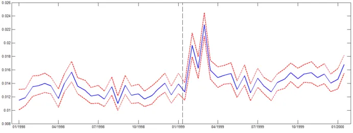
We start by showing results for non-tradable goods. They are expected to show little (or no) reaction to the currency devaluation shock and thus can be seen as a control group for this experiment. Figures 1 and 2 show the average magnitude and the probability of a positive price change from January 1998 till January 2000, respectively. In all figures, the vertical dotted line depicts the moment the exchange rate started to devalue (01/13/1999). The dotted lines are confidence intevals (estimates plus and minus two estimated standard errors), corresponding to a 5% confidence level. The results show that the pricing pattern of non-tradable goods is not significantly affected by the currency devaluation.9
Figure 1: Mean Size of Positive Price Changes: Non-Tradables
Figure 2: Probability of a Positive Price Change: Non-Tradables
Figure 3 shows the probability of a positive price change for industrialized goods. There is a clear spike following the devaluation shock, showing that the frequency of price changes
9
for industrialized goods strongly reacted to the devaluation. The probability of a positive change does not show any strong variation before January 1999, it swings between 1.1% and 1.4% a day for the whole year of 1998. Right after the devaluation, the probability goes up to around 2% a day.
Figure 3: Probability of a Positive Price Change: Industrialized goods
Figure 4 shows the magnitude of positive price changes for goods in the group of industri-alized goods. Interestingly, the devaluation episode seems to have no effect on the magnitude of price increases. If anything, there is a fall in the magnitude of price changes, but that fall is small and a similar pattern is observed in 1998.
Figure 4: Mean Size of Positive Price Changes: Industrialized goods
Differently from what time-dependent pricing models would predict, and in accordance to the predictions of state-dependent pricing models, the frequency of positive price changes was strongly affected by the devaluation shock of January 1999, while the magnitude of a devaluation was not significantly affected.10 Results thus match the strong predictions of a
10
A similar pattern is found in the group of commodities: the magnitude of price changes shows no discernible reaction, while the frequency of price changes shows a clear spike right after the devaluation episode.
simple Ss model along the lines of Caplin and Spulber (1987).
References
[1] Bonomo, Marco and Carvalho, Carlos V., 2004, “Endogenous Time-Dependent Rules and Inflation Inertia”,Journal of Money, Credit and Banking 36, 1015-1041.
[2] Calvo, Guillermo, 1983, “Staggered Contracts in a Utility Maximizing Framework”,
Journal of Monetary Economics 12, 383-98.
[3] Caplin, Andrew and Daniel Spulber, 1987, “Menu Costs and the Neutrality of Money”,
Quarterly Journal of Economics 102, 703-25.
[4] Gagnon, Etienne, 2009, “Price Setting During Low and High Inflation: Evidence from Mexico”, Quarterly Journal of Economics 124, 1221-1263.
[5] Gertler, Mark and John Leahy, 2008, “A Phillips Curve with an Ss Foundation”,Journal of Political Economy 116, 533-72.
[6] Golosov, Mikhail and Robert Lucas, 2007, “Menu Costs and Phillips Curves”, Journal of Political Economy 115, 171-199.
[7] Gouvea, Solange, 2007, “Price Rigidity in Brazil: Evidence from CPI Micro Data”, Working Paper 143, Banco Central do Brasil.
[8] Guimaraes, Bernardo; Mazini, Andre and Mendon¸ca, Diogo, 2014, “State-dependent or time-dependent pricing? Evidence from firms’ response to inflation shocks”, Working paper.
[9] Klenow, Peter and Kryvtsov, Oleksiy, 2008. “State-Dependent or Time-Dependent Pric-ing: Does It Matter for Recent U.S. Inflation?”, Quarterly Journal of Economics 123, 863-904.
A
Appendix
A.1 The devaluation of Brazilian Real
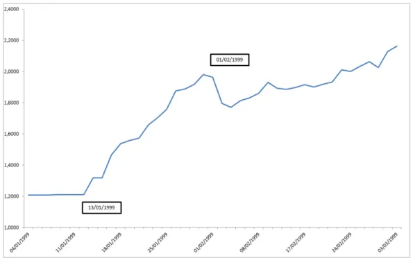
Between 1995 and January 1999, Brazil had a pegged regime: the currency was depreciating at an approximately constant rate of 0.6% a month. Figure 5 shows the Brazilian exchange rate in the first two months of 1999. The initial devaluation happened on the 13th
of January.
Figure 5: Exchange Rate: Beginning of 1999
The Brazilian government then tried to keep the devaluation at a level close to 10%, but that did not last more than 2 days. In the following 2 weeks, it gradually became clear the government had given up intervening in the foreign exchange market and a major devaluation took place.
A.2 Data: some descriptive statistics
Most items in the data set are in the group of tradables. In the tradable group, the majority of items are commodities. Items differ regarding the frequency of price collection. While non-tradables and industrialized goods have their prices collected, in average, every 26 and 28 days, respectively, commodities have a mean time of price collection of 12 days. In consequence, in terms of number of observations, tradables represent more than 90% of the whole sample. Nevertheless, there are almost 4000 non-tradable items and more than 8000 items in the group of industrialized goods.
Figure 6: Descriptive Statistics - Period Jan/98 till Jan/00
A.3 Commodities
The results for commodities are qualitatively similar to those from industrialized goods. Figure 7 shows the frequency of positive price changes in the group of commodities. Before January 1999, the probability of a price change in one day is roughly between 2% and 2.5%. Right after the devaluation shock, this probability raises to approximately 3%. Prices of commodities are in general very flexible. As in the case of industrialized goods, the average
Figure 7: Probability of a Positive Price Change: Commodities