Imperfectly Credible Disin
fl
ation under Endogenous
Time-Dependent Pricing
∗
Marco Bonomo
Graduate School of Economics, Getulio Vargas Foundation and CIREQ
Carlos Carvalho
Department of Economics
Princeton University
May 2006
Abstract
The real effects of an imperfectly credible disinflation depend critically on the extent of price rigidity. Therefore, the study of how policymakers’ credibility affects the outcome of an announced disinflation should not be dissociated from the analysis of the determinants of the frequency of price adjustments. In this paper we examine how the policymaker’s credibility affects the outcome of an announced disinflation in a model with endogenous time-dependent pricing rules. Both the initial degree of price ridigity, calculated optimally, and, more notably, the changes in contract length during disinflation play an important role in the explanation of the effects of imperfect credibility. We initially evalute the costs of disinflation in a setup where credibility is exogenous, and then allow agents to update beliefs about the “type” of monetary authority that they face. We show that, in both cases, the interaction between the endogeneity of time-dependent rules and imperfect credibility increases the output costs of disinflation.
JEL classification: E31; E52
1
Introduction
Lack of credibility has, for a long time, been pointed out as an important ingredient in explaining real effects of disinflation (e.g. Sargent, 1983). It arises when a monetary
authority that is serious about disinflating faces distrust from the private sector. Yet, price
rigidity is necessary for an imperfectly credible disinflation to have real effects. If prices
are fullyflexible, monetary policy essentially has no real effects, and the lack of credibility
does not matter.1 Furthermore, the real effects of an imperfectly credible disinflation will
depend on the extent of price rigidity.2
Consider an economy during an imperfectly credible disinflation in which individual
prices are fixed for very short periods of time. Then, the price optimally set by each agent
will tend to be very similar to the price that would be set under full credibility, since there is relatively little uncertainty about the monetary policy regime in the very short run. Therefore, the real effect of imperfect credibility will not be very important. However, the same will not be true for an economy where prices arefixed for long periods. Since policy
uncertainty tends to build up with time, there will be a much higher probability that the monetary authorities renege during this longer time period. Thus, the difference between the individual prices set during an imperfectly credible and a perfectly credible disinflation
becomes relevant, entailing important aggregate effects. As a result, credibility tends to have a more important role when the time period during which individual prices are kept
fixed is longer.
In this paper, our objective is to analyze how the policymaker’s credibility affects the outcome of an announced disinflation. For the reasons just outlined, this endeavor should
not be dissociated from the analysis of the determinants of the time interval between indi-vidual price adjustments. Therefore, we base our analysis on a model in which the period between individual adjustments, or contract length, is chosen optimally. This affects the impact of an announced disinflation. More importantly, changes in the contract lengths
during a disinflation, which can only be analyzed in a framework with endogenous pricing
rules, play an important role in the explanation of the effects of imperfect credibility. Credibility affects the costs of disinflation through a direct and an indirect effect on
prices. The direct effect is through the expectation of the optimal price during a given
1In standard models with one equilibrium. Of course, in a model with multiple equilibria, credibility,
as sunspots, may move the economy from one equilibrium to another.
2This applies to models where information about the optimal price is not continuously observed.
contract length, and appears in other models (e.g. Ball 1995, and Erceg and Levin 2003). The magnitude of this effect hinges on the duration of price contracts, as we argued before. Our approach allows us to calculate the optimal contract length corresponding to any initial inflationary steady state, and therefore to evaluate such direct effect appropriately.3
The indirect effect arises in our model with endogenous rules because changes in contract length during the disinflation also affect the individual prices chosen. With abrupt policy
shifts, as it happens with the announcement of a new disinflationary policy, this effect
becomes important.
The pricing rules are derived under the assumption that the price setter cannot obtain new information nor adjust prices based on her old information unless she incurs a lump sum cost, as in Bonomo and Carvalho (2004).4 As a result, optimal pricing rules are
endogenous time-dependent rules, where at each adjustment date the price setter chooses ex-ante when to adjust again. In choosing the optimal contract length, the price setter accounts for her beliefs about the likelihood of the disinflation being abandoned before
the next planned adjustment date.
We model imperfect credibility as a discrepancy between private agents’ beliefs about the likelihood that the monetary authority abandons the disinflation, and the objective
likelihood. For tractability, we assume that price setters believe that disinflation will be
abandoned with some constant hazard.
We examine initially the case where, despite price setters’ beliefs, the policymaker never reneges. We evaluate the output effects under exogenous and endogenous pricing rules. Our exogenous rules feature contract lengths which are chosen optimally for the inflationary environment which prevailed before the disinflation announcement. Thus, we
appropriately measure the direct effect of credibility by comparing the output effects of disinflation under perfect and imperfect credibility. As Ball (1995) points out, imperfect
credibility increases disinflation costs because agents believe that there is some probability
that the stabilization will be abandoned before their next adjustment date, and therefore set higher prices than in the full credibility case.
In order to assess the indirect effect, we examine the case in which pricing rules are endogenous, and compare it with the exogenous pricing rules case. We find that
endo-geneity of time-dependent rules increases the costs of imperfectly credible disinflation,
generating a larger recession when the stabilization is never abandoned. The intuition underlying the result is simple. With endogenous rules, price setters optimally choose
3When a contract length is chosen arbitrarily in a disin
flation exercise, the direct effect of credibility
will reflect this arbitrary choice.
4Ball, Mankiw, and Romer (1988) derive optimal contract lengths for inflationary steady states in a
longer contract lengths while the stabilization is maintained, and this raises the probabil-ity of abandonment occurring before the next adjustment date. Therefore, the difference between individual prices set under perfect and imperfect credibility becomes more im-portant. Endogeneity of pricing rules and imperfect credibility interact to generate an additional effect on top of the effects entailed by the endogeneity of rules under perfect credibility (Bonomo and Carvalho, 2004), and by imperfect credibility under exogenous rules (Ball, 1995).
The initial assumption that a disinflation is maintained indefinitely while the
discrep-ancy between agents’ beliefs and the resolve of the monetary authority remains unaltered, although useful for gaining insight in a simpler framework, is not plausible. It also gener-ates the unrealistic result that a certain level of recession goes on indefinitely. One should
expect that the monetary authority gains credibility through time, as agents update their beliefs about the resolve of the monetary authority by observing that disinflation
con-tinues. We handle this issue by endogenizing the evolution of agents’ beliefs through Bayesian learning. The result is a more realistic output path in which the monetary au-thority gains credibility, and the recession is gradually eliminated. Moreover, the main result of the paper, that endogeneity of pricing rules and lack of credibility interact to generate higher disinflation costs, continues to hold.5
The literature that links imperfect credibility and price rigidity explicitly starts with Ball (1995), who argues that both ingredients are necessary to explain the costs of
disin-flation. He focuses on average effects of disinflation when agents’ beliefs are in fact correct
(i.e. they know the distribution of abandonment times). Erceg and Levin (2003) try to explain the output costs during the Volcker disinflation in a model where agents have
to learn about a structural change in the interest rate rule. Both papers use exogenous pricing rules. Nicolae and Nolan (2006) model a credibility problem similar to ours, but have limited endogeneity of pricing rules: either prices are adjusted every period or every other period. They also introduce learning, but avoid Bayesian updating and, instead, ex-periment with alternative ad-hoc learning schemes.6 Finally, Almeida and Bonomo (2002)
and Golosov and Lucas (2005) analyze the effect of imperfect credibility using models of
5In an earlier version we also analyzed an alternative approach to reconcile agent’s beliefs with the
true probability that the monetary authority will renege. We followed Ball (1995) in assuming that the public’s beliefs reflect the objective probability that the monetary authority will renege. In this case
abandonment may occur at any date, and the outcome in which the disinflation is carried out to the end
is only a rare event. We calculated the effect of each possible abandonment realization and evaluated the average effect by weighting each individual path according to its likelihood. We found that endogeneity of pricing rules also increases the average costs of disinflation when agents’ beliefs are correct.
6Theyfind that imperfect credibility matters only under what they label “concave learning.” Bayesian
endogenous, state-dependent pricing rules. However, since price setters observe monetary policy continuously, imperfect credibility only has effect through the changes in pricing rules, and the real output effects are muted.7
The remaining part of the paper is organized as follows. In section 2 we present the model, and derive the optimal time-dependent rule under imperfectly credible disinflation.
Section 3 reports the aggregate effects obtained in our simulations of full and partial disinflation. Section 4 endogenizes credibility by assuming that agents use Bayes’ rule to
learn about the type of monetary authority that they face. The last section concludes.
2
The model
We depart from a model with a continuum of producers/consumers (yeoman farmers), each of whom produces a single variety of a consumption good, and derives utility from consuming a Dixit-Stiglitz composite of different varieties. Production entails disutility, which we assume to be subject to individual shocks. Those shocks can be interpreted either as a technological shock, or as a shock to preferences over labor/leisure. Each yeoman farmer is a price setter, and faces uncertainty over realizations of her revenue due to both the individual shock to disutility of producing and the conjunction of nominal price rigidity and staggering.8 All agents are, however, ex-ante identical, and we assume that
there exist state contingent markets which allow them to insure against such individual risks. As a result, they receive equal fractions offirms’ revenues. Under these assumptions
all agents face the same budget constraint at any point in time. As is now common in the literature, we assume a cashless economy (e.g. Woodford 2003).
In the appendix we develop the model from fundamentals, and derive the following loglinear expression for the frictionless optimal individual price of agent i,pit:
pit= (1−γ)pt+γ(Yt−ytn) +eit, (1)
wherept is the (log) aggregate price level,Yt is the (log) nominal aggregate demand,ytnis
the (log) natural output rate. Theeit’s are mutually independent zero mean idiosyncratic
7There is another line of investigation about the effects of imperfect credibility on disinflation, which
is to explain the determinants of policymakers’ choices of monetary policy and of the initial gap between the public’s beliefs and the policymaker’s resolve to disinflate. Those models usually assume that prices
are rigid for only one period, and rely on the discretionary nature of monetary policy. A recent example is Westelius (2005). Backus and Driffill (1985a,b) provided earlier contributions.
8Individual shocks to disutility of producing will make agents choose different production levels, which
components of the individual shocks to the disutility of producing (see appendix).
In (1), 1−γ is the degree of strategic complementarity in price setting, and is re-lated to primitive parameters such as the elasticity of substitution between varieties (see appendix). Individual prices are strategic complements (substitutes) if γ <1(>1).9
In order tofind the aggregate price in a frictionless equilibrium, we integrate (1) across
all agents:
pt=Yt−ytn.
Thus, aggregate output and individual prices are given by yn
t and pit = pt +eit,
respectively.
For simplicity, in the subsequent sections we abstract from aggregate shocks, which implies that natural output is constant. Thus, all variation of the output level will be attributed to output gap variation as a result of price rigidity.
2.1
Optimal time-dependent pricing rule
Gathering and processing information about the optimal price, and making price ad-justments are costly activities. We assume that agents can neither observe the stochastic components of their optimal frictionless price process nor adjust prices based on its known components without incurring a utility cost. Every time an agent decides to get informa-tion and/or adjust its price she loses a small fracinforma-tion of her lifetime utility. So, the optimal pricing policy amounts to choosing a sequence of information gathering/adjustment times and prices to be set at those times. In the appendix, we show that a suitable approx-imation to this optimal pricing problem can be characterized by the following Bellman equation:10
Vt= min
zt,τt
Et
∙Z τt
0
(zt−(pit+s−pit))2e−ρsds+e−ρτt(F +Vt+τt)
¸
. (2)
Here, F is the fraction of utility that is lost at each adjustment,11 τt denotes the time
until the next adjustment, and zt denotes the discrepancy between the price set at t,xit,
and its frictionless optimal level:12
zt≡xit−pit. (3)
9Ball and Romer (1990) argued that the possible strategic complementarities in price setting re flect
rigidities of desired relative prices to changes in quantities.
10We drop theisubscript from choice variables to simplify notation.
11To be precise, it is the fraction of utility that is lost, normalized by the concavity of the profit
function. See the appendix for a formal definition.
12We will refer toz
The first order conditions are:
zt∗ = ρ 1−eρτ∗t
Z τ∗
t
0
e−ρsEt(pit+s−pit)ds, (4)
and
Et £
zt∗−¡pit+τ∗t −pit
¢¤2
−ρF −ρEtVt+τ∗t +
∂EtVt+τ∗
t
∂t = 0. (5)
Equations (2), (4), and (5) fully characterize the optimal pricing rule, as long as the second order conditions are satisfied.
2.2
In
fl
ationary steady state
In analyzing disinflations we start from an inflationary steady state characterized by a
constant rate of inflation. Letµbe the constant growth rate of nominal aggregate demand.
If we differentiate equation (1), and use the assumption of contant natural output rate and the fact that in steady state all prices grow at the same rate, we obtain:
dpit =µdt+deit. (6)
Realistically we think ofei as being a very persistent, but stationary process.13
How-ever, modeling it as a mean-reverting process would add a new state variable to the model without changing the main insights. Thus, we adopt the Brownian motion as a convenient approximation of its short run dynamics, that is:
deit =σdWit,
where Wit’s are mutually independent standard Brownian motions.
Given these assumptions, the Bellman equation (2) becomes time invariant:14
Vµ = min
z,τ Et
∙Z τ
0
(z−(pit+s−pit))2e−ρsds+e−ρτ(F +Vµ) ¸
, (7)
where Vµ represents the value function for the steady state problem with nominal
aggre-13If it were non-stationary, individual variables could deviate arbitrarily from their steady state values
in the long run, undermining the validity of our approximations.
14In steady state, the value function and the optimalz andτ will be the same for all agents, because
gate demand growth rate equal to µ. The first order conditions (4) and (5) become:15
z∗ = ρ 1−e−ρτ∗
Z τ∗
0
Et(pit+s−pit)e−ρsds; (8)
Et[z∗−(pit+τ∗−pit)]2−ρ(Vµ+F) = 0. (9)
Manipulating (6), (7), (8), and (9), we arrive at the following equations, which define τ∗
implicitly, and z∗:
ρ Rτ∗
0
µ µ2³h1
ρ − e−ρτ∗
1−e−ρτ∗τ∗
i
−s´2+σ2s
e−ρsds+F
1−e−ρτ∗ =µ 2
µ
1
ρ −
e−ρτ∗
1−e−ρτ∗τ∗ −τ∗
¶2
+σ2τ∗;
z∗ =µ µ
1
ρ −
e−ρτ∗
1−e−ρτ∗τ∗
¶ .
Based on the above pair of equations, one can show that the optimal contract length is decreasing in |µ| and σ, increasing in F, and is not affected by the degree of strategic
complementarity, 1−γ. In addition, higher idiosyncratic uncertainty makes the optimal
contract length less sensitive to inflation (Bonomo and Carvalho 2004).
In our simulations, we set σ = 3% and calibrate F in such a way that with µ= 3%,
σ = 3% and ρ = 2.5% a year, agents choose to keep prices fixed for a year. As a result
we set F = 0.000595. This adjustment interval seems to be a reasonable characterization of price setting behavior in low inflation environments. It is consistent with thefindings
of Dhyne et al. (2005) for the Euro area, and with earlier evidence for the U.S. economy (e.g. Carlton, 1986 and Blinder et al., 1998), although it is longer than the average length reported by Bils and Klenow (2004) for the U.S. economy.
In order to check the robustness of our calibration, we also computed the optimal contract length for high and very high inflation rates. The model performs well when
confronted with the Israeli experience reported by Lach and Tsiddon (1992),16 and it also
fits the Brazilian hyperinflation experience of the 80’s (Ferreira, 1994). With inflation
rates of 77% per year the model predicts contract lengths of 2.6 months, against 2.2 months reported by Lach and Tsiddon (1992), and with annual inflation of 210% the
theoretical contract length goes down to 1.68 months, against 1.38 months reported by Ferreira (1994).
2.3
Optimal pricing rule under imperfectly credible disin
fl
ation
In this subsection we derive optimal pricing rules during disinflation. In general, this
requires solving both an optimization and an aggregation problem simultaneously. This is because the optimal rule depends on the expected path for the aggregate price level, which in turn results from the aggregation of the individual pricing rules. In the absence of strategic complementarities (γ = 1) these problems can be solved sequentially.
We simplify the analysis by assuming away strategic complementarities. This is a common assumption in state-dependent pricing models, where aggregation can be cum-bersome (e.g. Caplin and Leahy 1991, Almeida and Bonomo 2002, and Golosov and Lucas 2005). In terms of primitives of our model this obtains if, for instance, utility is logarithmic in consumption and the disutility of production is linear.17
The dynamic program formulated in (2) encompasses imperfect credibility in general, which enters the problem through the expectations operator. It is more realistic to assume that agents believe that there is some probability that the new disinflation policy will be
abandoned, than to assume full credibility. We model imperfect credibility by positing that in each finite time interval agents attribute a constant probability of abandonment.
Thus, from the agents’ perspective, the growth rate of nominal aggregate demand after the announcement changes with the first arrival of a Poisson process with constant rate
h. In case of abandonment, agents believe that the old policy is resumed and maintained forever.18
Despite agents’ beliefs, we assume in this section that the monetary authority never reneges. Therefore, after the stabilization policy is launched at t= 0, the actual process
for Yt is given by:
dYt = µ0dt;
Y0 = 0,
where µ0 is the targeted growth rate for nominal aggregate demand. We refer to the case
of µ0 = 0 as “full disinflation,” while µ > µ0 > 0 corresponds to a “partial disinflation.”
17For a thorough discussion of how strategic complementarity relates to primitives in general
equilib-rium models see Woodford (2003, ch. 3). See also Huang and Liu (2002).
18We abstract from issues of recurring regime changes, as discussed in Cooley et al. (1984). In this
case, optimal contract lengths during the inflationary steady state should also incorporate the possibility
We implicitly assume that the monetary authority sets its policy instruments so as to generate the postulated disinflation path for nominal aggregate demand.
However, nominal aggregate demand according to agents’ beliefs,Yb
t, evolves as:
dYtb = (µ0+ (µ−µ0) 1{Nt>1})dt; Y0b = 0,
whereNtis a Poisson counting process with constant arrival rateh, and1{·}is the indicator
function.
With this formulation we can interpreth as a measure of credibility, with high values
representing low credibility. The subjective probability that stabilization will last until time T is given by e−hT. Thus, for example, if h = 0.5, the subjective probability that
the stabilization will continue after one year is 61%. The polar cases of perfect and no credibility correspond to h= 0 and h=∞, respectively.
The problem of an agent while the stabilization has not been abandoned may be written as:
Vh = min
z,τ £
Gh(z, τ) +e−ρτ¡F +e−hτVh+¡1−e−hτ¢Vµ¢¤, (10)
where
Gh(z, τ) ≡ e−hτ
∙Z τ
0
³
(z−µ0s)2+σ2s´e−ρsds ¸
+ (11)
Z τ
0
" Rr
0
¡
(z−µ0s)2+σ2s¢e−ρsds+ Rτ
r ¡
(z−µ(s−r)−µ0r)2 +σ2s¢e−ρsds #
he−hrdr.
In (10), Gh(z, τ) is the expected cost due to deviations from the frictionless optimal
price during the next interval of length τ, starting with the discrepancy z. Observe that
if abandonment occurs during the next contract, agents will not learn of it until the new adjustment date,19’20 when the new contract will be set under conditions identical to the
inflationary steady state. This results in the cost functionVµ. In (11), thefirst line of the
expression refers to the subjective probability that the stabilization will be kept during the next contract multiplied by the cost in this case. The second line is the discrepancy cost if abandonment occurs at time t+r weighted by the (subjective) likelihood of this
19In Bonomo and Carvalho (2004), agents are allowed to reevaluate their pricing policies when the
disinflation is announced. They conclude that the changes in the results can be important for high
but not for low inflation environments. We conjecture that a similar conclusion obtains with respect to
abandonment under imperfect credibility, for the same reasons outlined in that paper.
20Furthermore, it seems reasonable to assume that the news of abandonment does not become freely
event.
The first order conditions are derived in a straightforward way:21
z∗ = ρ 1−e−ρτ∗
Z τ∗
0
∙
µ0s+ (µ−µ0)
µ
s− 1−e−
hs h
¶¸
e−ρsds; (12)
(z∗−µ0τ∗)2
+σ2τ∗+he−hτ∗(V
µ−Vh)−ρF −ρ ¡
e−hτ∗V h+
¡
1−e−hτ∗¢V µ
¢
(13)
+
Z τ∗
0
((µ0−µ) (τ∗−r))2he−hrdr+ 2 (µ0−µ) (z∗−µ0τ∗)
Z τ∗
0
(τ∗−r)he−hrdr = 0.
From (12), (13), (10), (11) and (7), we obtain a nonlinear equation in τ∗, which can
be solved numerically.
Figure 1 shows the optimal contract length as a function of the credibility level in a full disinflation, for two levels of initial inflation (µ= 0.1and µ= 0.2). As expected, the
higher h is (the lower the credibility level), the shorter the contract length is.
3
Aggregate results
3.1
Aggregation methodology
With endogenous pricing rules, contract lengths change during disinflation, and the
dis-tribution of adjustments times changes accordingly. Aggregation requires tracking those changes, and must be done numerically. Knowledge of the optimal contract length at each point in time enables us to relate the relevant distribution for aggregation at each moment to distributions at preceding times. We proceed recursively until we arrive at the known inflationary steady state distribution, which we assume to be uniform.
3.2
Results
We start by illustrating how optimal contract lengths might be relevant for the direct effect of imperfect credibility, in Figures 2 and 3. In Figure 2, we compare the output effects of perfectly and imperfectly credible disinflations,fixing the same arbitrary contract
length for two different initial inflation rates.22 It is apparent that the direct effect is
more important for higher inflation rates. The reason is that, given the same contract
length, agents set higher prices because of the risk of facing higher inflation in case the
21Again, the second order conditions are satisfied.
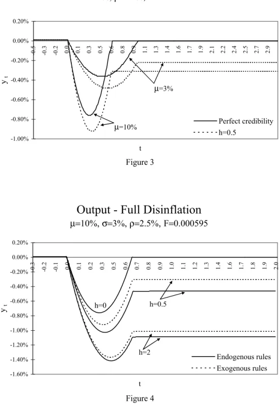
stabilization is abandoned before their next adjustment date. In Figure 3, on the other hand, contract lengths are fixed at the optimal level for each initial inflation rate. The
relation between inflation and the direct effect of imperfect credibility is now unclear. The
reason is that contract lengths are shorter for higher initial inflation rates and so, despite
the fact that inflation would be higher in the case of abandonment, the probability that
this event happens before the next adjustment date is now smaller.
These results illustrate how important it is to use the appropriate contract length to evaluate the direct effect of imperfect credibility. Therefore, in all of our subsequent ex-periments, we fix the contract length under exogenous rules at the optimum for the initial
inflationary steady state. In our view, this is the right assumption for the experiments
we analyze, which are unexpected disinflations. We start from an inflationary steady
state which is expected to last, and so it makes sense to use contract lengths which are compatible with that steady state. This allows us to properly assess the indirect effect of imperfect credibility, by appropriately taking the direct effect into account.
Figure 4 depicts the output effects of a full disinflation with our baseline calibration
for two levels of credibility (h = 0.5, and h = 2), with both endogenous and exogenous
rules. The case of perfect credibility (h = 0) is presented for comparison purposes. As
expected, with imperfect credibility the recession generated is larger. It is clear that endogeneity of pricing rules reinforces this result. This happens because contract lengths increase after disinflation. With perfect credibility, as shown in Bonomo and Carvalho
(2004), in the case of full disinflation and no strategic complementarities, the output costs
of disinflation are the same with endogenous or exogenous rules. The reason is that every
agent which adjusts after disinflation is announced knows that the aggregate component
of their optimal price will remain constant. Then, individual prices are set taking into account only the idiosyncratic component of the optimal price, and contract lengths have no aggregate impact. With imperfect credibility this result ceases to be true, since agents attribute some probability that the monetary authority will abandon the stabilization before their next adjustment, in which case inflation will resume. With endogenous rules,
prices are fixed for a longer interval when compared with the exogenous rules case, which
implies a higher (subjective) probability of abandonment before the next price adjustment. Therefore, prices are set at higher levels and the recession is larger. This is a result of the interaction between imperfect credibility and endogeneity of contract lengths.
If credibility is lower contract lengths increase less after the disinflation is announced,
In Figure 5 we explore the role of idiosyncratic uncertainty. In the case of a perfectly credible full disinflation, idiosyncratic shocks are required for optimal contract lengths to
befinite after the announcement. Otherwise, with zero inflation and no uncertainty, there
would be no reason to collect information or change prices.23 With imperfect credibility,
however, this is no longer the case, since the possibility of abandonment leads agents to chose finite contract lengths irrespective of idiosyncratic uncertainty. The lower σ
is, the more optimal contract lengths are sensitive to inflation.24 So, when σ = 0 the
differences between the endogenous and the exogenous rules cases are amplified, because
agents choose relatively longer contract lengths. This comparison is illustrated in Figure 5, against our benchmark value σ = 3%.
These results on the effects of different levels of credibility and idiosyncratic uncer-tainty illustrate important general features of the interaction between imperfect credibility and endogeneity of contract lengths, which also apply to the other results that we present. To avoid having too many simulations, however, we chose to illustrate them only through the previous experiments.
A partial disinflation presents some qualitative differences when compared to a full
disinflation. The reason is that, with nominal rigidity in individual prices, the expected
discrepancy while there is no individual price adjustment only remains constant when the inflation drift is zero. So, in contrast with the full disinflation case, in a partial disinflation
a longer contract length will induce agents to set higher prices even with full credibility. With partial disinflation and imperfect credibility, continuing inflation and the
probabil-ity of reneging interact with the contract length to affect pricing decisions. Given the optimally chosen longer contract length, firms incorporate both the (higher) probability
of abandonment and ongoing inflation when setting their prices. As a consequence, the
recession tends to be larger.
Figure 6 shows the result of a partial disinflation under imperfect credibility for both
exogenous and endogenous rules. As expected, the endogenous rule model generates a larger recession, but also output cycles. These cycles result from gaps in the new distribution of adjustment times, which are generated by the sudden increase in contract lengths.25
23This issue does not arise when in
flation is always strictly positive, in which case idiosyncratic
uncer-tainty can be dispensed with. Conlon and Liu (1997) explore this fact in a menu cost model with a two dimensional optimal pricing rule.
24This is true both in the inflationary steady state, and during disinflation.
25Note that those gaps also occur in the case of full disinflation. However, they cause no output
4
Disin
fl
ation with learning
The results analyzed so far correspond to a situation in which the monetary authority never reneges, but nevertheless agents continue to believe that there is always the same probability of abandonment. Thus, the recession continues indefinitely, which is clearly
unrealistic.
This result arises from the conjunction of two assumptions: initial beliefs that do not correspond to the true type of the monetary authority,26 and lack of updating of such
beliefs as disinflation evolves.
Discrepancies between agents’ beliefs and the actual type of the monetary authority capture the essence of the problem faced by a monetary authority that is really serious about disinflating, but has low credibility. Lack of updating of beliefs, on the other hand,
is clearly an extreme and unrealistic assumption, which we drop in this section.
We analyze how credibility evolves during disinflation, and how this interacts with
price setting and with endogeneity of time-dependent rules to determine the output costs of disinflation. Initially, all agents hold the same beliefs about the type of the monetary
authority that they face. After the disinflation is announced, every time an agent collects
information she also updates her beliefs about the type of the monetary authority, taking into account whether or not disinflation has been abandoned. Updating is done according
to Bayes’ rule.
In the next subsection we present the framework with learning, and derive the optimal pricing rule. We then specialize to the case of a monetary authority who is fully committed to disinflate, but initially lacks credibility. We compare the costs of disinflation under both
endogenous and exogenous pricing rules.
4.1
Optimal pricing rule
We assume that there are two possible types for the monetary authority, characterized by the constant hazard rate for the Poisson process according to which it reneges:27 h > h > 0. We assume that when the disinflation policy is announced at t = 0, agents
have the same belief about the type of monetary authority they face. We denote by πthe prior probability of the monetary authority being of type h.
At any time t > 0, whenever agents update their information sets, they observe
whether disinflation has been abandoned and, conditional on no abandonment, form the
26We interpret has indexing the possible behavioral types that the monetary authority can assume.
For instance, a monetary authority that never reneges is of type h= 0.
posterior πt, according to Bayes’ rule:28
πt ≡ Pr{h=h|Nt= 0}
= Pr{h=h, Nt = 0}
Pr{h=h, Nt = 0}+ Pr©h=h, Nt= 0ª
= πe
−ht
πe−ht+ (1−π)e−ht.
While there is no abandonment, the optimization problem of an agent adjusting/collecting information at time t is given by:
Vtπ = min
zt,τt
"
πtGh(zt, τt) + (1−πt)Gh(zt, τt) + e−ρτt³F +³π
te−hτt + (1−πt)e−hτt ´
Vπ t+τt +
³
1−³πte−hτt + (1−πt)e−hτt ´´
Vµ ´
# .
(14) We solve the above problem numerically, as described in the appendix.
4.2
Results
We focus on the case of a monetary authority that is fully committed to disinflate (i.e., of
type h= 0) but faces a credibility problem at the time of the disinflation announcement
(h >0, π <1).
Figure 7 presents the path for the optimal contract length during a full disinflation.
When the disinflation is announced att= 0, agents who get to collect information and ad-just at that time choose tofix prices for longer periods when compared to the inflationary
steady-state, and therefore optimal contract lengths jump. As the disinflation evolves, the
monetary authority gains credibility and agents who adjust subsequently choose progres-sively longer contracts. In the limit, ast→ ∞, agents end up believing that the monetary authority is actually not going to renege, and so optimal contract lengths approach their optimal zero inflation level.
The paths for output under both endogenous and exogenous pricing rules are presented in Figure 8. They share the general features of the full disinflation case without learning
(Figure 4), with one noticeable exception: now, as credibility builds up, output reverts towards the steady state level. Once more, the recession is larger under endogenous pricing rules.
The differences between these results and the ones for a full disinflation without
learn-28Agents also update their beliefs when they learn that the disinflation has been abandoned. However,
ing hinge on the process of updating of beliefs. According with our assumptions, every time an agent collects information she also updates her beliefs about the type of the monetary authority she faces. Because agents choose different contract lengths and are staggered in terms of their information collection/adjustment times, at each point in time there is an endogenously determined distribution of beliefs, which can be represented by
{πi t}
1
i=0, where πit ≡ Pr{h=h|Nti = 0}, and ti represents the time when agent i last
collected information and adjusted her price.
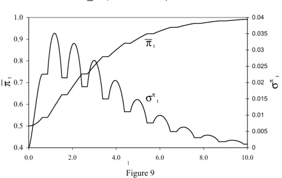
We summarize the evolution of this distribution of beliefs during disinflation by its
mean (πt ≡ R01π
i
tdi) and standard deviation (σπt ≡ qR1
0 (πit−πt)
2
di), which we present
in Figure 9. When the disinflation is announced all agents hold the same belief, given
by the common prior π. As disinflation evolves, agents who get to adjust update their
beliefs upwards, and therefore the average belief increases at the same time asσπ
t starts to
indicate dispersion in the corresponding distribution. This process continues for a while, with beliefs becoming more dispersed as agents choose longer contracts and update at different times, until a point in which the tendency reverts and beliefs start to converge, albeit non-monotonically. Meanwhile, the average belief increases steadily towards unity.
5
Conclusion
The role of credibility in monetary disinflations depends critically on the extent of price
rigidity. This paper evaluates the effect of imperfect credibility of the disinflation policy
in a model in which the time period between individual price adjustments is chosen optimally ex-ante. As a result we are able to evaluate both the direct effect of credibility, for a given frequency of price adjustments, and the indirect effect, which is engendered by the endogeneity of price setting rules. The latter is important, as the effects of imperfect credibility and endogeneity of pricing rules interact. When the model is augmented with learning, it generates a realistic output pattern for the disinflation process. Those results
References
[1] Almeida, H. and M. Bonomo (2002), “Optimal State-Dependent Rules, Credibility and Inflation Inertia,” Journal of Monetary Economics 49: 1317-1336.
[2] Backus, D. and J. Driffill (1985a), “Rational Expectations and Policy Credibility Following a Change in Regime,” Review of Economic Studies 52: 211-221.
[3] Backus, D. and J. Driffill (1985b), “Inflation and Reputation,”American Economic Review 75: 530-538.
[4] Ball, L. (1995), “Disinflation with Imperfect Credibility,”Journal of Monetary Eco-nomics 35: 5-23.
[5] Ball, L. and G. Mankiw (1994), “Asymmetric Price Adjustment and Economic Fluc-tuations,” Economic Journal 104: 247-261.
[6] Ball, L., N. G. Mankiw and D. Romer (1988), “The New Keynesian Economics and the Output-Inflation Trade-off,” Brookings Papers on Economic Activity 1: 1-65.
[7] Ball, L. and D. Romer (1990), “Real Rigidities and the Non-Neutrality of Money,”
Review of Economic Studies 57: 183-203.
[8] Bils, M. and P. Klenow (2004), “Some Evidence on the Importance of Sticky Prices,”
Journal of Political Economy 112: 947-985.
[9] Blinder, A., E. Canetti, D. Lebow, and J. Rudd (1998), Asking about Prices: A New Approach to Understanding Price Stickiness, Russel Sage Foundation.
[10] Bonomo, M. and C. Carvalho (2004), “Endogenous Time-Dependent Rules and
In-flation Inertia,” Journal of Money, Credit and Banking 36: 1015-1041.
[11] Caplin, A. and J. Leahy (1991), “State-Dependent Pricing and the Dynamics of Money and Output,” Quarterly Journal of Economics 106: 683-708.
[12] Caplin, A. and D. Spulber (1987), “Menu Costs and the Neutrality of Money,” Quar-terly Journal of Economics 102: 703-726.
[13] Carlton, D. (1986), “The Rigidity of Prices,” American Economic Review 76:
[14] Conlon, J. and C. Liu (1997), “Can More Frequent Price Changes Lead to Price Iner-tia? Nonneutralities in a State-Dependent Pricing Context,”International Economic Review 38: 893-914.
[15] Cooley, T., S. Leroy and N. Raymon (1984), “Econometric policy evaluation: note,”
American Economic Review 74: 467-70.
[16] Dhyne, E., L. Álvarez, H. Le Bihan, G. Veronese, D. Dias, J. Hoffman, N. Jonker, P. Lünnemann, F. Rumler and J. Vilmunen (2005), “Price Setting in the Euro Area: Some Stylised Facts from Individual Consumer Price Data,” ECB Working Paper Series no. 524.
[17] Erceg, C. and A. Levin (2003), “Imperfect Credibility and Inflation Persistence,”
Journal of Monetary Economics 50: 915-944.
[18] Ferreira, S. (1994), “Inflação, Regras de Reajuste e Busca Sequencial: Uma
Abor-dagem sob a Ótica da Dispersão de Preços Relativos,” M.A. Dissertation, PUC-Rio.
[19] Golosov, M. and R. Lucas (2005),“Menu Costs and Phillips Curves,” mimeo.
[20] Huang, K. and C. Liu (2002), “Staggered Price-Setting, Staggered Wage-Setting, and Business Cycle Persistence,” Journal of Monetary Economics 49: 405-433.
[21] Lach, S. and D. Tsiddon (1992), “The Behavior of Prices and Inflation: An Empirical
Analysis of Disaggregated Price Data,” Journal of Political Economy 100: 349-389.
[22] Mankiw, G., and R. Reis (2002), “Sticky Information Versus Sticky Prices: A Pro-posal to Replace the New Keynesian Phillips Curve,”Quarterly Journal of Economics
117: 1295-1328 .
[23] Nicolae, A. and C. Nolan (2006), “The Impact of Imperfect Credibility in a Transition to Price Stability,” Journal of Money, Credit, and Banking 38: 47-66.
[24] Reis, R. (2006), “Inattentive Producers,” forthcoming in the Review of Economic Studies.
[25] Sargent, T. (1983), “Stopping Moderate Inflations: The Methods of Poincare and
Thatcher,” in: Dornbusch, R. and M. Simonsen (eds.), Inflation, Debt and Indexa-tion, MIT Press, Cambridge, MA.
[27] Taylor, J. (1980), “Aggregate Dynamics and Staggered Contracts,” Journal of Polit-ical Economy 88: 1-23.
[28] Westelius, N. (2005), “Discretionary Monetary Policy and Inflation Persistence,”
Journal of Monetary Economics 52:477-496.
Appendix A
Here we derive the frictionless optimal price in an general equilibrium framework with both aggregate and idiosyncratic shocks.
Each yeoman farmer, indexed byi, maximizes the following utility function:29
Et0
∙Z ∞ 0
e−ρ(t−t0)[u(Ct)−v(Yit, εit)]dt ¸
,
where
Ct≡
∙Z 1 0
Citθ−θ1di
¸ θ θ−1
,
with θ > 1, and Pt is defined by
Pt≡
∙Z 1 0
Pit1−θdi ¸ 1
1−θ
, (15)
subject to the corresponding (continuum of) budget constraints:
dAt =
µ itAt+
Z 1
0
PjtYjtdj−
Z 1
0
PjtCjtdj+Tt 
dt, fort ≥t0,
and a no-Ponzi condition:
lim
s→∞A(s)e
−Utsirdr ≥0.
In the above equations, εit is an individual shock to the disutility of producing good i, Cit is the consumption of goodi,Pit is its price, Yit its supply,it is the net interest rate
on financial wealthAt, andTt is the net lump-sumflow transfer from the government.
Individual shocks are decomposed as
εit =εt+ξit,
where εt is the aggregate shock given by εt ≡ R1
0 εitdi, and ξit is an idiosyncratic shock.
We assume that idiosyncratic shocks have the same law of motion for all agents, and are mutually independent.
29We assume thatu(·)is strictly concave and increasing, and that v(·, ε
it)is strictly increasing and
It is straightforward to show that, in this setting, the demand for an individual product has the following familiar relation with aggregate demand:
Cit =
µ Pit
Pt ¶−θ
Ct. (16)
Underflexible prices, each producer chooses the supply of its good to maximize utility.
The corresponding first order condition is:
µ Yt Yit
¶1
θ
= θ
θ−1s(Yit, Yt, εit), (17)
where we have used the equilibrium condition Yt = Ct, and s(Yit, Yt, εit) is the implicit
real marginal cost of producing Yit:
s(Yit, Yt, εit) = vy(Yit, εit)
uc(Yt) .
In this economy a flexible price equilibrium is characterized by a valid equation (17)
for each i andYt given by:30
Yt≡
∙Z 1 0
Y θ− 1
θ
it di ¸ θ
θ−1
. (18)
We define the level of natural output Yn
t as the aggregate output level corresponding to the flexible price equilibrium. This is similar to the standard concept in the literature
(e.g. Woodford, 2003, chapter 3). However, notice that here each individual output level in general differs from Yn
t due to the existence of idiosyncratic shocks.
Proceeding analogously as in Woodford (2003), we define the steady state level of
production,Y, as the output level in the symmetricflexible price equilibrium whenεit= 0
for all i. So, it satisfies:
1 = θ
θ−1s
¡
Y , Y ,0¢.
In order to obtain a more explicit characterization of theflexible price equilibrium we
loglinearize both sides of equation (17) around steady state levels and rearrange to get:
b yit =
1−θλ
1 +θωbyt− θ
1 +θω it, (19)
30Equations (17) and (18) de
fine implicitly a functionΨ:³{Yjt}j6=i , εit
´
→Yit. For a given realization
εit, defineΨit
³
{Yjt}j6=i
´
≡Ψ³{Yjt}j6=i, εit
´
. For given realizationsεitfor alli, an equilibrium is afixed
wherebyit ≡log¡Yit
Y ¢,
b
yt≡log¡Yt
Y ¢,
it ≡
∂logs(Y ,Y ,0)
∂εi εit=
∂logvy(Y;0)
∂εi εit,ω≡
∂logs(Y ,Y ,0)
∂logyi =
∂logvy(Y ,0)
∂logyi , and λ≡ −
∂loguc(Y)
∂logY .
Loglinearizing (18), and using (19), we obtain a relation between the natural output rate and the aggregate shock:
b
ytn=−(ω+λ)−1 t, (20)
where ybn t ≡log
³Yn t
Y ´
, and t≡
∂logvy(Y;0)
∂εi εt.
In order to derive a relation between the individual optimal price and the output gap, we first loglinearize the demand function:31
b
yit =byt−θ(pit−pt), (21)
where pit ≡logPit, and pt≡logPt.
Then, we substitute (21) into (19) to get:
pit−pt=
ω+λ
1 +θωybt+
1 1 +θω it.
Finally, we decompose itinto its aggregate and idiosyncratic components and use (20)
to replace t, obtaining:
pit−pt =γ(yt−ynt) +eit, (22)
where yt≡logYt, yn
t ≡logYtn,eit≡ 1+1θω( it− t), and γ ≡ ω+λ
1+θω >0.
Since our focus is on the supply side of the model, we take (log) nominal aggregate demand{Yt}t=0 to be an exogenous process. Substituting yt≡Yt−ptinto (22) we arrive
at an expression for the frictionless optimal price:
pit= (1−γ)pt+γ(Yt−ytn) +eit. (23)
Appendix B
Here we formulate the original optimal price setting problem and show that an ap-proximation leads to the problem presented in the main text. We assume that agents can neither observe the stochastic components of their optimal price process nor adjust prices based on its known components without incurring a utility cost. Every time an agent decides to get information and/or adjust its price she loses a small fraction of her lifetime utility. To solve for the optimal price setting policy, we make the usual assumption that she maximizes intertemporal profits, valued with the pricing kernel obtained from the first order conditions for optimal consumption. The optimal pricing policy amounts to
choosing a sequence of adjustment times (tj’s) and prices to be set at those times (Xtj’s)
to maximize such intertemporal profits.
LetVit0e be the value function associated with the production activity of agenti
imme-diately after incurring the information/adjustment cost at a time t0, but before choosing
Xt0:
e
Vit0 = max
{tj},{Xtj},j≥1,Xt0 Et0
"̰ Y
j=1
1−e−ρ(tj−t0)Fe
!
ϕ³{tj}∞j=0,©Xtj
ª∞
j=0
´#
, (24)
where tj is a time of adjustment/information gathering, Xtj is the price chosen at time
tj, ande−ρ(tj−t0)Fe denotes the fraction of utility that is lost due to adjustment attj. The
function ϕ(·,·) is given by:
ϕ³{tj}∞j=0,©Xtjª∞j=0´ ≡
∞
X
j=0
e−ρ(tj−t0)uc
¡ Ctj
¢
uc(Ct0) ×
tj+1Z−tj
0
e−ρsuc ¡
Ctj+s
¢
uc¡Ctj
¢ Π¡Xtj, Ptj+s, Ytj+s, εitj+s
¢ ds,
where
Π(X, P, Y, ε) = X
P µ
X P
¶−θ Y −v
õ X P
¶−θ Y, ε
! .
For comparison purposes we define the frictionless value functionVeit∗as the value
func-tion associated with the producfunc-tion activity when there are no adjustment/informafunc-tion costs:
e
Vit∗ =Et
∞
Z
0
e−ρ(s−t)uc(Ct+s)
It is convenient to reestate (24) as an equivalent problem in terms of the difference between the frictionless value function and the value function with frictions:
Vit0 ≡ logVeit0∗ −logVeit0
= min
{tj},{Xtj},j≥1,Xt0
⎧ ⎪ ⎪ ⎪ ⎪ ⎪ ⎪ ⎪ ⎨ ⎪ ⎪ ⎪ ⎪ ⎪ ⎪ ⎪ ⎩ log µ Et0 ∞ R 0
e−ρ(s−t0)uc(Ct0+s) uc(Ct0)
Π(Pit0+s, Pt0+s, Yt0+s, εit0+s)ds 
−P∞
j=1
log(1−e−ρ(tj−t0)Fe)
−log à Et0 ∞ P j=0
e−ρ(tj−t0)
tj+1R−tj
0
e−ρs uc(Ctj+s)
uc(Ct0)
Π¡Xtj, Ptj+s, Ytj+s, εitj+s
¢ ds ! ⎫ ⎪ ⎪ ⎪ ⎪ ⎪ ⎪ ⎪ ⎬ ⎪ ⎪ ⎪ ⎪ ⎪ ⎪ ⎪ ⎭ ' min
{tj},{Xtj},j≥1,Xt0
⎧ ⎪ ⎪ ⎪ ⎪ ⎪ ⎪ ⎨ ⎪ ⎪ ⎪ ⎪ ⎪ ⎪ ⎩ ⎡ ⎢ ⎢ ⎢ ⎢ ⎢ ⎢ ⎣ ∞ P j=0
e−ρ(tj−t0)Fe+Et0 ∞
P j=0
e−ρ(tj−t0)
tj+1R−tj
0
e−ρs×
⎧ ⎪ ⎪ ⎨ ⎪ ⎪ ⎩ log ∙
uc(Ctj+s)
uc(Ct0)
Π¡Pitj+s, Ptj+s, Ytj+s, εitj+s
¢¸
−log
∙
uc(Ctj+s)
uc(Ct0)
Π¡Xtj, Ptj+s, Ytj+s, εitj+s
¢¸ ⎫ ⎪ ⎪ ⎬ ⎪ ⎪ ⎭ ds ⎤ ⎥ ⎥ ⎥ ⎥ ⎥ ⎥ ⎦ ⎫ ⎪ ⎪ ⎪ ⎪ ⎪ ⎪ ⎬ ⎪ ⎪ ⎪ ⎪ ⎪ ⎪ ⎭ = min
{tj},{Xtj},j≥1,Xt0 Et0
∞
X
j=0
e−ρ(tj−t0)
⎧ ⎪ ⎪ ⎪ ⎨ ⎪ ⎪ ⎪ ⎩
e−ρ(tj+1−tj)Fe+
tj+1R−tj
0
e−ρs× "
log¡Π¡Pitj+s, Ptj+s, Ytj+s, εitj+s
¢¢
−log¡Π¡Xtj, Ptj+s, Ytj+s, εitj+s
¢¢ # ds ⎫ ⎪ ⎪ ⎪ ⎬ ⎪ ⎪ ⎪ ⎭ ' min
{tj},{xtj},j≥1,xt0 Et0
∞
X
j=0
e−ρ(tj−t0)
⎧ ⎨ ⎩e
−ρ(tj+1−tj)Fe+
tj+1Z−tj
0
e−ρsαtj+s
¡
xtj −pitj+s
¢2
ds
⎫ ⎬ ⎭,
where xt≡logxt, αtj+s≡ −12
∂2logΠ(p
itj+s,Ptj+s,Ytj+s,εitj+s)
∂x2 >0.
The last step follows from a second order approximation aroundxtj =pitj+s, for alls.
If αtj+s=α, a constant, and defining F ≡ h
F
α, this is equivalent to:
min
{tj},{xtj}
Et0
∞
X
j=0
e−ρ(tj−t0)
⎡ ⎣
tj+1Z−tj
0
e−ρs¡xtj−pitj+s
¢2
ds+e−ρ(tj+1−tj)F
⎤ ⎦
Using the definition of discrepancy (3), and rewriting the above problem in recursive
Appendix C
Here we present the solution method for (14). The corresponding first order conditions are:
z∗t = ρ 1−e−ρτ∗t
Z τ∗
t
0
"
µ0s+ (µ−µ0)
à s−
Ã
πt1−e− hs
h + (1−πt) Ã
1−e−hs h
!!!#
e−ρsds;
(25)
(z∗t −µ0τ∗t)2+σ2τt∗+³πthe−hτ∗t + (1−πt)he−hτ∗t
´ ³
Vµ−Vtπ+τ∗
t
´
+ (26)
³
πte−hτ∗t + (1−πt)e−hτ∗t
´∂Vπ t+τ∗
t
∂t −ρ ³
F +Vµ+³πte−hτt∗+ (1−πt)e−hτ∗t
´ ³ Vtπ+τ∗
t −Vµ
´´
+
Z τ∗
t
0
((µ0−µ) (τ∗t −r))2³πthe−hr+ (1−πt)he−hr´dr+
2 (µ0−µ) (z∗
t −µ0τ∗t) Z τ∗
t
0
(τ∗t −r)³πthe−hr+ (1−πt)he−hr ´
dr= 0.
Equations (25), (26), and (14) characterize zt∗, τ∗t and Vπ t+τ∗
t. To solve this set of
equations, wefirst pickT large enough, such that, for t > T, Vπ
t can be taken as
approx-imately constant. This is justified: conditional on no abandonment, the probability that
the monetary authority is of typeh keeps increasing, and the problem becomes more and
more similar to the one analyzed in section (2.3), with h = h. Formally, lim
t→∞πt = 1,
32
which implies that lim
t→∞V
π t+τ∗
t = Vh. So, we solve the set of equations moving backwards
in time. For each t we findz∗
t, τ∗t and use them to computeVtπ, which will then be used
to find z∗, τ∗ at earlier times. Alternatively, to avoid numerical derivatives, one can use
(25), and (14) tofindτ∗
t with a grid search, instead of using (26). This is the method we
adopted.
32Just rewriteπ
t as 1
1+(1−ππ)e−(h−h)t
Obs: Contract lengths are fixed at the level corresponding to the optimum for µ=3%. Figure 1
Figure 2
Optimal Contract Length - Full Disinflation
σ=3%, ρ=2.5%,F=0.0005950.2 0.3 0.4 0.5 0.6 0.7 0.8 0.9 1 1.1 1.2
0.0 1.0 2.0 3.0 4.0 5.0 6.0 7.0 8.0 9.0 10.0
τ
∗
h µ=10%
µ=20%
Direct Effect - Arbitrary Contract Lengths
Different Initial Inflation Rates - Full Disinflation
σ=3%,ρ=2.5%, F=0.000595
-1.80% -1.60% -1.40% -1.20% -1.00% -0.80% -0.60% -0.40% -0.20% 0.00% 0.20%
-0
.5
-0
.3
-0
.2 0.0 0.1 0.3 0.5 0.6 0.8 0.9 1.1 1.3 1.4 1.6 1.7 1.9 2.1 2.2 2.4 2.5 2.7 2.9
t
y t
Perfect credibility h=0.5
µ=3%
Figure 4 Figure 3
Output - Full Disinflation
µ=10%, σ=3%,ρ=2.5%, F=0.000595-1.60% -1.40% -1.20% -1.00% -0.80% -0.60% -0.40% -0.20% 0.00% 0.20%
-0
.3
-0
.2
-0
.1 0.0 0.1 0.2 0.3 0.5 0.6 0.7 0.8 0.9 1.0 1.1 1.2 1.3 1.4 1.6 1.7 1.8 1.9 2.0
t
y t
Endogenous rules Exogenous rules
h=0 h=0.5
h=2
Direct Effect - Optimal Contract Lengths
Different Initial Inflation Rates - Full Disinflation
σ=3%,ρ=2.5%, F=0.000595
-1.00% -0.80% -0.60% -0.40% -0.20% 0.00% 0.20%
-0
.5
-0
.3
-0
.2 0.0 0.1 0.3 0.5 0.6 0.8 0.9 1.1 1.3 1.4 1.6 1.7 1.9 2.1 2.2 2.4 2.5 2.7 2.9
t
y t
Perfect credibility h=0.5
µ=3%
Figure 5
Figure 6
Output - Partial Disinflation
µ=10%, µ'=2%, h=0.5, σ=3%, ρ=2.5%, F=0.000595
-1.00% -0.80% -0.60% -0.40% -0.20% 0.00% 0.20%
-0
.3
2
-0
.1
5
0.03 0.20 0.38 0.55 0.72 0.90 1.07 1.25 1.42 1.59 1.77 1.94
y t
Endogenous rules
Exogenous rules
t
Output - Full Disinflation
µ=10%, h=0.5,ρ=2.5%, F=0.000595-1.25% -1.05% -0.85% -0.65% -0.45% -0.25% -0.05% 0.15%
-0
.3
-0
.2
-0
.1 0.0 0.1 0.2 0.3 0.5 0.6 0.7 0.8 0.9 1.0 1.1 1.2 1.3 1.4 1.6 1.7 1.8 1.9 2.0
t
y t
Endogenous rules Exogenous rules h=0
σ=3%
Figure 7
Figure 8
Optimal Contract Length with Learning
π=0.5, h=0.5, h=0, µ=10%, σ=3%, ρ=2.5%, F=0.000595
0.40 0.50 0.60 0.70 0.80 0.90 1.00 1.10 1.20
-5.0 0.0 5.0 10.0 15.0 20.0
τ
tt
Output - Disinflation with Learning
π=0.5, h=0.5, h=0, µ=10%, σ=3%, ρ=2.5%, F=0.000595
-1.00% -0.80% -0.60% -0.40% -0.20% 0.00% 0.20%
-1.0 0.0 1.0 2.0 3.0 4.0 5.0
y t
t
Figure 9
Evolution of Beliefs
π=0.5, h=0.5, h=0, µ=10%, σ=3%, ρ=2.5%, F=0.000595
0.4 0.5 0.6 0.7 0.8 0.9 1.0
0.0 2.0 4.0 6.0 8.0 10.0
π
t
0 0.005 0.01 0.015 0.02 0.025 0.03 0.035 0.04
σ
π
t
t