UNIVERSIDADE TÉCNICA DE LISBOA INSTITUTO SUPERIOR DE ECONOMIA E GESTÃO

(1)

UNIVERSIDADE TÉCNICA DE LISBOA

INSTITUTO SUPERIOR DE ECONOMIA E GESTÃO

Evaluation of ruin probabilities for surplus processes

with credibility and surplus dependent premiums

Maria de Lourdes Belchior Afonso

(Mestre)

Dissertação para obtenção do Grau de Doutor em Matemática Aplicada à Economia e Gestão

Orientação:

Doutor Alfredo Duarte Egídio dos Reis Doutor Howard Richard Waters

Júri

Presidente: Reitor da Universidade Técnica de Lisboa Vogais: Doutor João Tiago Praça Nunes Mexia

(2)

(3)

(4)

(5)

Acknowledgements

Apart from staring at 200 blank pages at the beginning of the writing process, this

is the most difficult part to write. There were many people, from the tallest (Nelson) to the shortest (Mariana), who supported me in several ways during the past three and half

years.

My first thoughts are for my supervisors Professor Alfredo Eg´ıdio dos Reis and Pro-fessor Howard Waters for their generous support, valuable guidance and specially for their

friendship during this project. Many thanks for having accepted me as a Ph.D. student.

I’ve increased my knowledge in so many different areas.

I would like to thank Professor Jo˜ao Tiago Mexia for introducing me to the academic

career. I am grateful to Centro de Matem´atica e Aplica¸c˜oes of FCT/UNL for the financial

support for my working visits to Heriot-Watt University and to present part of this work at the IME 2007 conference, to Funda¸c˜ao Calouste Gulbenkian for financial support to

present part of this work at the IME 2006 conference, to Faculdade de Ciˆencias e Tecnologia

and CEMAPRE-ISEG for allowing me to use their servers to run the C++ programs. I would also like to thank two people whom I know only through e-mail, Dr. Kenneth

Wilder of the University of Chicago for helping me to change his C++ random number

(6)

To my friends Ana Lu´ısa Batista, Carolann Waters, David Pontes, F´atima Miguens, Isabel Gomes, Gracinda Guerreiro, Pedro Corte Real, Rui Cardoso, Teresa Afonso, Vitor

Chagas and all the others who are not mentioned here, I thank you for your support and

specially for your friendship.

My utmost gratitude goes to my parents who encouraged me and made every possible

effort to support me in whatever way they could, without having the slightest idea of

the meaning of ruin theory or credibility theory. From all my heart I’m grateful to my daughter Mariana (who was born at the beginning of this project) and my husband Nelson,

to whom I proudly dedicate this work. They have taught me the meaning of unconditional

love.

Despite all the work involved in the project, the bad nights sleep, the extra white

hairs, all the chips, popcorn and chewing gum eaten, I must confess that I had much fun,

(7)

Resumo

´

E proposto um m´etodo para o c´alculo da probabilidade de ruina em tempo cont´ınuo e

horizonte finito para um processo de Poisson composto onde o pr´emio ´e constante ao longo

de cada per´ıodo de tempo (ano), mas depende da informa¸cão passada de indemniza¸cões agregadas anuais. Em fun¸cão disso, o prémio é ajustado anualmente, passando a ser

vari´avel de per´ıodo para per´ıodo.

Um dos grandes contributos deste trabalho é o facto da metodologia apresentada ser facilmente aplicável a carteiras de grande dimensão. O método é baseado na simula¸cão das

indemniza¸c˜oes agregadas anuais e no calculo da probabilidade de ru´ına dado um determi-nado montante de reserva no in´ıcio e no fim do per´ıodo. Este c´alculo da probabilidade de

ru´ına ´e aproximado de duas formas: primeiro usando um movimento Browniano adequado

e depois uma aproxima¸cão à distribui¸cão gama deslocada.

A coerˆencia dos resultados produzidos pelo modelo ´e testada comparando os resultados

produzidos para o modelo cl´assico de risco com o modelo-base e com os resultados exactos

obtidos por Wikstad (1971) e por Seal (1978), em tempo cont´ınuo e horizonte finito.

O método é aplicado a três modelos de risco diferentes em que o prémio é actualizado

no ´ınicio do ano. Para cada modelo as indemniza¸c˜oes agregadas seguem uma distribui¸c˜ao

(8)

No primeiro modelo o prémio é definido como fun¸cão do n´ıvel de reserva em algum momento anterior. O coeficiente de carga para o prémio anual é determinado em cada

caso de forma `a probabilidade em horizonte infinito, partindo da reserva incial considerada,

ser aproximadamente um valor pré-definido para o modelo clássico. Para tal, é utilizada a aproxima¸cão de De Vylder (1978). No segundo e terceiro modelos considera-se uma

carteira que satisfaz as hip´oteses dos modelos de credibilidade de B¨uhlmann e B¨

uhlmann-Straub sendo o pr´emio anual actualizado de acordo com estes modelos.

Palavras-Chave: _{Probabilidade de Ru´ına, Movimento Browniano,}

Apro-xima¸cão à Gama deslocada, Simula¸cão, Prémios dependentes da reserva, Prémios de

(9)

Abstract

In this dissertation we present a method for the numerical evaluation of the ruin

prob-ability in continuous and finite time for a classical risk process where the premium can change from year to year. A major consideration in the development of this methodology

is that it should be easily applicable to large portfolios. Our method is based on the simu-lation of the annual aggregate claims and then on the calcusimu-lation of the ruin probability for

a given surplus at the start and at the end of each year. We calculate the within-year ruin

probability assuming first a Brownian motion approximation and, secondly, a translated gamma distribution approximation for aggregate claim amounts.

We will check the accuracy of our method by comparing our results applied to the

classical risk process with the results of Wikstad (1971) and Seal (1978b) in finite and

continuous time. We also check its accuracy in the case of exponential and mixed expo-nential claim amounts by choosing a very long time horizon and comparing results with

exact results for infinite time ruin.

We apply our method to three different risk models where the premium is set at the start of each year but can change from year to year. For each model aggregate claims have

a compound Poisson distribution with either a fixed or a variable Poisson parameter for

(10)

probability of ultimate ruin from that time is approximately equal to a pre-determined value. We will use De Vylder’s (1978) approximation to achieve that. For the second

and third models we consider a portfolio of risks which satisfy the assumptions of the

B¨uhlmann or B¨uhlmann-Straub credibility models with the pure premium updated each year in accordance with these models.

Keywords:_{Ruin probabilities, Brownian motion approximation, translated gamma}

(11)

List of Tables

2.1 Values and estimates of ψ(u, n): Exponentially distributed claim

amounts. Seal (1978b). . . 16

2.2 Values and estimates of ψ(u, n): Exponentially distributed claim amounts. Wikstad (1971). . . 17

2.3 Values and estimates of ψ(u, n): Swedish fire insurance claim amounts. Wikstad (1971). . . 18

2.4 Values and estimates of ψ(u): Exponentially distributed claim amounts. Gerber (1979). . . 20

2.5 Values and estimates ofψ(u): Individual claim amounts being a mix-ture of exponentials. Gerber (1979). . . 21

3.6 Pairs (ζ, u): Lognormal claims, ω = 0.01. . . 26

3.7 Mean, variance and skewness: Exponential, lognormal and gamma. . 28

3.8 Exponential: Parameters for the power function for formula (3.19). . 30

3.9 Exponential: Safety loading obtained by De Vylder’s formulavs fitted power function. . . 30

3.10 Exponential: Values for ψ(u) calculated using De Vylder’s formula and safety loadings of Table 3.9. . . 31

3.11 Exponential: Estimates and standard deviations of ψ(u,10), T1 N1. . 31

3.15 Exponential: Statistical information for ruin cases, T1 N1. . . 35

3.16 Exponential: Statistical information for ruin cases, T1 N2. . . 36

3.17 Exponential: Correlation between yi and yi−1. . . 39

3.18 Lognormal: Parameters for the power function for formula (3.19). . . 45

3.19 Lognormal: Safety loading obtained by De Vylder’s formula vs fitted power function. . . 45

3.20 Lognormal: Values forψ(u) calculated using formula (3.18) and safety loading (3.19). . . 46

3.21 Lognormal: Estimates and standard deviations of ψ(u,10), T1 N1. . . 46

3.24 Lognormal: Estimates and standard deviations of ψ(u,10), T2 N2. . 47

3.25 Lognormal: Statistical information for ruin cases, T1 N1. . . 49

3.26 Lognormal: Statistical information for ruin cases, T1 N2. . . 50

3.27 Lognormal: Correlation between yi and yi−₁. . . 52

(14)

3.29 Gamma: Safety loading obtained by De Vylder’s formula vs fitted

power function. . . 57

3.30 Gamma: Values for ψ(u) calculated using formula (3.18) and safety loading (3.19). . . 58

3.31 Gamma: Estimates and standard deviations of ψ(u,10), T1 N1. . . . 58

3.35 Gamma: Statistical information for ruin cases, T1 N1. . . 61

3.36 Gamma: Statistical information for ruin cases, T1 N2. . . 62

3.37 Gamma: Correlation between yi and yi−₁. . . 64

3.38 Values of ψT G(u,10 000): λ = 1. . . 71

3.39 Values of ψT G(u,10 000): λ ∼U[0.8,1.2]. . . 71

3.40 Estimates of ruin probabilities for Michaud’s and for our methodologies. 72 4.41 B¨uhlmann: Distribution of Θ. . . 82

4.42 B¨uhlmann: Parameters for the power function for formula (3.19). . . 82

4.43 B¨uhlmann: Safety loading obtained by De Vylder’s formulavs fitted power function and respective values for ψ(u). . . 83

4.44 One run: Translated gamma parameters. . . 84

4.45 One run: Aggregate claims and credibility factor for year i. . . 85

4.46 One run: Pure premiums in year i. . . 86

4.47 One run: Premiums in year i. . . 87

4.48 One run: Surplus at the end of year i. . . 88

4.49 One run: Ruin probabilities ψT G(u(i−1),1, u(i)) and ψT G(u,10). . . 89

4.50 B¨uhlmann: Estimates and standard deviations of ψ(u,10), N1. . . 91

4.51 B¨uhlmann: Estimates and standard deviations of ψ(u,10), N2. . . 92

4.52 B¨uhlmann: Statistical information for ruin cases, N1 u= 250. . . 95

4.56 Bühlmann: Statistical information for ruin cases for the portfolio, N1. 99 4.57 Bühlmann: Statistical information for ruin cases for the portfolio, N2. 100 4.58 Bühlmann: Percentage of ruined risks due to ruined portfolio. . . 102

4.59 B¨uhlmann: Correlation betweenyi−1 and yi. . . 103

4.60 B¨uhlmann: Common ruin scenarios. . . 104

4.61 B¨uhlmann: Statistics for the credibility factor. . . 105

5.62 B¨uhlmann-Straub: Risk volume by case W, risk and year. . . 116

5.63 B¨uhlmann-Straub: Estimates and standard deviations of ψ(u,10), W1 per risk with equal surplus. . . 119

5.64 B¨uhlmann-Straub: Estimates and standard deviations of ψ(u,10), W1 per risk with rated surplus. . . 120

5.65 B¨uhlmann-Straub: Estimates and standard deviations ofψ(u,10), N1 W1. . . 122

5.66 B¨uhlmann-Straub: Estimates and standard deviations ofψ(u,10), N2 W1. . . 122

(15)

5.68 B¨uhlmann-Straub: Estimates and standard deviations ofψ(u,10), N2 W2. . . 123 5.69 B¨uhlmann-Straub: Estimates and standard deviations ofψ(u,10), N1

W3. . . 123 5.70 B¨uhlmann-Straub: Estimates and standard deviations ofψ(u,10), N2

W4. . . 125 5.73 Bühlmann-Straub: Statistical information for ruin cases, W1 N1. . . . 126 5.74 Bühlmann-Straub: Statistical information for ruin cases, W1 N2. . . . 127 5.75 Bühlmann-Straub: Statistical information for ruin cases, W2 N1. . . . 128 5.76 Bühlmann-Straub: Statistical information for ruin cases, W2 N2. . . . 129 5.77 Bühlmann-Straub: Statistical information for ruin cases, W3 N2. . . . 130 5.78 Bühlmann-Straub: Statistical information for ruin cases, W4 N1. . . . 131 5.79 Bühlmann-Straub: Statistical information for ruin cases, W4 N2. . . . 132 5.80 Bühlmann-Straub: Correlation betweenyi−₁ andy_i, for combinations

of W1, W2, N and P. . . 134 5.81 B¨uhlmann-Straub: Correlation betweenyi−1 andyi, for combinations

(16)

(17)

List of Figures

3.1 Fitted power function: Lognormal claims,ω = 0.01. . . 27

3.2 Cdf: Exponential, lognormal and gamma. . . 28

3.3 Exponential: ψ(u,10) for several values of initial surplus. . . 40

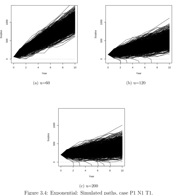
3.4 Exponential: Simulated paths, case P1 N1 T1. . . 42

3.7 Lognormal: ψ(u,10) for several values of initial surplus. . . 53

3.8 Lognormal: Simulated paths, case P1 N1 T1. . . 54

3.11 Gamma: ψ(u,10) for several values of initial surplus. . . 65

3.12 Gamma: Simulated paths, case P1 N1 T1 . . . 66

4.15 B¨uhlmann: Time axis. . . 83

4.16 B¨uhlmann: ψ(u,10) for several values of initial surplus. . . 104

4.17 B¨uhlmann: Statistics for the credibility factor. . . 105

4.18 B¨uhlmann: Simulated paths, case N1, u= 300. . . 106

5.19 B¨uhlmann-Straub: Evolution of the risk volume along the years by risk. . . 118

5.20 B¨uhlmann-Straub: ψ(u,10) for several values of initial surplus, W1. . 136

5.24 B¨uhlmann-Straub: Simulated paths, case W1 N2, u= 90. . . 138

5.25 B¨uhlmann-Straub: Simulated paths, case W2 N1, u= 90. . . 139

(18)

(19)

Chapter 1 Introduction

The aim of this thesis is to present a method for calculating the probability of

ruin in finite time for a compound Poisson risk process where the premium rate

is constant throughout the year but depends on the past aggregate annual claims

experience and hence changes each year.

Ruin theory has its roots in the beginning of the twentieth century when

fun-damental ideas were published by Lundberg (1903). Since then many studies have

dealt with the exact or approximate computation of ruin probabilities, mainly for

the classical risk process.

The problem of calculating the probability of ruin when the premium is a function

of the surplus level at the end of the year has been studied by many authors, in

most of the cases in infinite time. For example, Davidson (1969) let the safety

loading decrease with an increasing risk reserve. Taylor (1980) and Jasiulewicz

(2001) consider the case where the premium rate varies continuously as a function

of the surplus. Petersen (1989) illustrates with a simple numerical method how the

probability of ruin can be calculated when the general premium rate depends on the

reserve. Dickson (1991) considers the case where the premium rate changes when

the surplus crosses an upper barrier. More recently, Cardoso and Waters (2005)

presented a numerical method for calculating finite time ruin probabilities for the

same problem.

(20)

Mowbray (1914) raised the question of what premium should be used if the

individ-ual risk experience for a single contract is found to be insufficient. Whitney (1918)

suggested using a weighted average of the individual and collective premium as a

solution. Most authors have the opinion that it was B¨uhlmann who supplied a

the-oretical background to this problem in his papers B¨uhlmann (1967) and B¨uhlmann

(1969). B¨uhlmann and Straub (1970) recognised that contracts often have different

underlying risk exposures and extended B¨uhlmann’s model.

The problem of calculating the probability of ruin for a risk process where the

pre-mium is updated according to a credibility model was considered by Dubey (1977)

and Tsai and Parker (2004). The former contains some interesting theoretical

re-sults; the latter paper is focused on numerical results for a discrete time model where

the premium is updated according to the B¨uhlmann credibility model.

The use of simulation to estimate ruin probabilities is not new. Dufresne and

Gerber (1989) observe that the probability of ruin is related to the stationary

dis-tribution of a certain associated process and estimate it using simulation. Michaud

(1996) simulated the jumps and interjump times for two models in order to

approx-imate the probability of ultapprox-imate ruin. In his first model the surplus earns interest;

in his second model the premium depends on the level of the surplus.

Our method involves simulating the aggregate claims for each year, calculating

the premium to be charged each year given the past aggregate claim amounts, and

then calculating the within year probability of ruin assuming either a Brownian

motion approximation to the surplus process or a translated gamma distribution

approximation for aggregate claim amounts. The Brownian motion approximation

is well established, see for example Sections 8.6 and 8.7 of Klugman et al. (2004), and

should work well if the expected number of claims in each year is reasonably large.

The translated gamma approximation uses ideas which go back to Seal (1978a) and

which have recently been used by Dickson and Waters (2006). We would expect the

latter approximation to be better than the former since it is based on three rather

than two moments.

(21)

probabilities in finite time which we will use in the following chapters. Details of

the approximations and of our simulation procedure are given. We will check the

accuracy of our method by comparing our results applied to the classical risk process

with the results of Wikstad (1971) and Seal (1978b) in finite and continuous time.

We also compare our results with the results for ultimate ruin probabilities in cases

where claim amounts are exponentially distributed and where they are a mixture of

exponentials (Gerber (1979)).

In Chapter 3 we consider the problem of calculating the probability of ruin for

a risk process where the premium is set at the start of the year. We consider the

premium calculated according to the level of surplus at the beginning of the year.

In practice it may not be possible to achieve this since there may be some delay

between the end of the year and the new premium being introduced. For this reason

we consider the case where the premium in the coming year depends on the surplus

one year ago. We also consider the classical case where the premium depends on

the initial surplus and is constant throughout the remaining period. The premium

rate is set in each case so that the probability of ultimate ruin from that time is

approximately equal to a pre-determined value (0.005 or 0.01). We will use De

Vylder’s (1978) approximation to achieve that.

Chapter 4 is a step forward. We deal with the calculation of the probability of

ruin for a portfolio of risks where the premium for each individual risk is updated

each year based on the experience for all the risks according to the B¨uhlmann

cred-ibility model. In order to understand the impact of the credcred-ibility premium on the

ruin probability we will consider also the premium calculated using the conditional

expected value of the aggregate claim amount. The safety loading will be calculated

using the same approach as in the previous chapter. The methodology is similar to

the one used before with some minor adjustments.

In Chapter 5 we consider the B¨uhlmann-Straub credibility model. This model

allows for variation in exposure or size. In this chapter we will use a fixed safety

loading and compare the results using the B¨uhlmann-Straub credibility premium

with the ones using the conditional expected value of aggregate claims.

(22)

classical one (constant throughout the period) and a varying one.

Numerical examples are discussed at the end of each chapter. Figures and

statis-tics are shown to make it easier to understand the results. Some conclusions and

comments on further research are set out in Chapter 6.

Much of the work of Chapters 2 and 3 of this thesis is presented in the paper by

Afonso et al. (2007a), and the work of Chapters 4 and 5 is presented in the paper

(23)

Chapter 2 The basic algorithm

In this Chapter we set out our model and general procedure for the numerical

evaluation of the ruin probability in continuous and finite time for a classical risk

process where the premium can change from year to year. Our method is based on

the simulation of the annual aggregate claims and then on the numerical calculation

of the ruin probability for a given surplus at the start and at the end of each year. We

calculate the within-year ruin probability assuming first a Brownian motion process

approximation and, secondly, a translated gamma distribution approximation.

In Section 2.1 we set out our model and general procedure for calculating ruin

probabilities in continuous and finite time. In Sections 2.2 and 2.3 we give details of

the Brownian motion and the translated gamma approximations we use to calculate

the probability of ruin within each year, given the surplus at the start and at the

end of the year. Details of our procedure to simulate ruin probabilities are given

in Section 2.4. Wikstad (1971) and Seal (1978b) give values for the probability of

ruin in finite and continuous time for some examples of a classical risk process (with

constant premiums). In Section 2.5 we check the accuracy of our methodology

by applying it to these examples and comparing our values with theirs. We also

compare our results for a long period, say 1 000 years, with the results of Gerber

(1979) for the ultimate ruin probability when claim amounts have an exponential

(24)

also be found in Bowers et al. (1997) (Example 13.6.2). Finally in Section 2.6 we

set out some conclusions.

2.1 The model

With no loss of generality consider time to be measured in years. Consider a risk

process over an n-year period which is described by

U(t) = u+

i−₁

X

j=1

Pj+ (t−i+ 1)Pi−S(t), 0≤t ≤n (2.1)

wherei is such that t_∈[i₋1, i), i= 1,2, ..., n, and where

0

X

j=1

Pj = 0.

U(t) is the insurer’s surplus at time t, 0_≤t_≤n,

u is the insurer’s initial surplus (=U(0)) and is assumed to be known,

Pi is the premium charged in yeari, where year imeans time i−1 to i,

S(t) is the aggregate claims up to time t so that S(0) = 0.

We defineYi =S(i)−S(i−1),i= 1,2, . . . , nso thatYi is the aggregate claims in

year i. We assume that _{Yi}ni=1 is a sequence of i.i.d. random variables, each with

a compound Poisson distribution whose first three moments exist. This assumption

will be modified in Chapters 4 and 5 to allow the distribution of aggregate claims

to depend on the value of a risk parameter,θ, say.

{S(t)_}∞

t=0is assumed to be a compound Poisson process. The Poisson parameter,

and hence the expected number of claims each year, is λ.

We also assume that premiums are received continuously at a constant rate

throughout each year and that the initial premium,P1, is known. For i= 2, . . . , n,

we assume that Pi is a function of {Yj}i

−₁

j=1, the aggregate claims in the preceding

years and is updated at the beginning of the year.

Fori_≥2, the premiumPi and surplus level U(i) are random variables since they

(25)

a particular realisation of these variables, we will use the lower case letters pi and

u(i).

The probability of ruin in continuous time within n years is denoted by ψ(u, n) and defined as:

ψ(u, n)def= Pr(U(t)<0 for some t_∈(0, n])

Letψ(u(i₋1),1, u(i)) be the probability of ruin within year i, given the surplus

u(i₋1) at the start of the year and the surplusu(i) at the end. To approximate this probability we will use Brownian motion process and translated gamma distribution

approximations.

2.2 The Brownian motion process approximation

In this section we give an approximation, using a Brownian motion process with

drift, to calculate the ruin probability within one year, given the surplus at the start

and at the end of the year.

Definition 2.2.1 A continuous-time stochastic process _{W(s);s _≥0_} is a Brown-ian motion process with drift coefficientµ and variance per unit timeσ2 _if:

(i) W(0) = 0;

(ii) _{W(s);s_≥0_} has stationary and independent increments;

(iii) W(s) is normally distributed (with mean µsand variance σ2_s_).

Let_{W(s);s_≥0_}be a Brownian motion process. For the given valuesu(i₋1) and

pi, we approximate the surplus process, {U(t)}over the time interval i−1 ≤t≤ i

(26)

µ=pi−E[Yi] and σ2 = Var[Yi]

so that for 0_≤s (=t₋i+ 1)_≤1:

E[u(i₋1) +W(s)] =u(i₋1) +s(pi−E[Yi]) = E[U(t)|U(i−1) =u(i−1)]

Var[u(i₋1) +W(s)] =σ2s= Var[U(t)]_|U(i₋1) =u(i₋1)] Let T denote the time until ruin for this approximating process, so that:

T = inf(s >0 :u(i₋1) +W(s)<0)

with the convention that T = _∞ if ruin never occurs. Klugman et al. (2004), Corollary 8.25, show that the probability that ruin ever occurs, denoted

ψBM(u(i−1)), is:

ψBM(u(i−1)) = exp

µ

−2µu(_σi2−1)

¶

(2.2)

and in Corollary 8.27 show that the probability density of the time to ruin, given

that ruin occurs, denotedfT(s), is:

fT(s) =

u(i₋1)

√

2πσ2 s

−₃_/₂

exp³₋ (u(i−1)−µs)

2

2σ2_s

´

, s >0 (2.3) Hence, the probability density of the time to ruin, for finites, without conditioning on whether ruin occurs, is the product of (2.2) and (2.3), that is:

fT(s)ψBM(u(i−1)) =

u(i₋1)

√

2πσ2 s

−₃_/₂

exp³₋(u(i−1)−µs)

2_{+ 4}_µsu₍_i₋₁₎

2σ2_s

´ (2.4)

Klugman et al. (2004) also show (page 259) that, for 0< s <1, the conditional probability density of u(i₋1) +W(1) at y, given that T =s, denoted f(y_|T =s), is:

f(y_|T =s) = exp³yµ

σ2

´exp³₋ y2+µ2(1−_s₎2

2σ2₍₁−_s₎ ´

p

2πσ2₍₁₋_s₎ (2.5)

Hence, for 0 < T < 1, the joint probability density of u(i₋1) +W(1) and T is given by the product of (2.4) and (2.5) and the conditional probability density ofT, given thatu(i₋1) +W(1) =u(i), denotedfW(s), is the product of (2.4) and (2.5)

(27)

fW(s) =

exp³u(i)µ

σ2

´_u₍_i₋₁₎_s−3/2

2πσ2

1 √

1−sexp ³

−u(i)

2₊_µ2₍₁₋_s₎2

2σ2₍₁₋_s₎ −

(u(i−1)−µs)2

2σ2_s −

2µu(i−1)

σ2

´

n(u(i)−u(i−1), µ, σ2₎

where n(_·, µ, σ2_{) is the density function of the normal distribution.}

Finally, the probability of ruin in the year, given that the surplus at the end of

the year is u(i), is given by the integral of this last conditional density from s = 0 tos= 1. We denote this probability ψBM(u(i−1),1, u(i)), so that:

ψBM(u(i−1),1, u(i)) =

Z 1

s=0

fW(s)ds (2.6)

For now on we will use ψBM(u(i − 1),1, u(i)) as an approximation to

ψ(u(i₋1),1, u(i)).

2.3 The translated gamma distribution

approxi-mation

We now return to the (compound Poisson) surplus process, _{U(t)_} described in (2.1). We consider the time interval [i₋1, i) and we assume we know the history of the process up to time i₋1. Hence, the premium income in the year, pi, is known.

We are interested in ψ(u(i₋1),1, u(i)), the probability of ruin within the year given the starting and final values for U(t). We will develop a formula for

ψ(u(i₋1),1, u(i)) following methods in Dickson and Waters (2006, Section 3.2). Let ∆(u(i₋1),1, y) denote the probability that, starting from a surplus ofu(i₋1), ruin does not occur in the year and the surplus at the end of the year is greater

than y. Let f(_·, s) and F(_·, s) denote the density function and the distribution function of the aggregate claims in a time interval of length s. Then:

∆(u(i₋1),1, y) = Z ∞

y

(1₋ψ(u(i₋1),1, z))f(u(i₋1) +pi−z,1)dz

and so:

ψ(u(i₋1),1, y) = 1 + 1

f(u(i₋1) +pi−y,1)

d

(28)

Let δ(u(i₋1), t, y)dy denote the probability that, starting from initial surplus

u(i₋1), ruin does not occur before time t and the surplus at time t is between y

and y+dy. Then:

δ(u(i₋1), t, y) =₋ d

dy∆(u(i−1), t, y)

Using formula (3.13) from Dickson and Waters (2006):

δ(u(i₋1),1, y) = f(u(i₋1) +pi−y,1)−f(u(i−1) +pi−y,1−y/pi) exp(−λy/pi)

−pi

Z 1−y/p_i

s=0

f(u(i₋1) +pis, s)δ(0,1−s, y)ds

and formula (3.11) from the same reference:

δ(0, t, y) = y

pit

f(pit−y, t)

and writingy =u(i) we have:

ψ(u(i₋1),1, u(i)) =

R1−_u₍_i₎_/p_i

s=0 f(u(i−1) +pis, s)

u(i)

(1−_s₎f(pi(1−s)−u(i),1−s)ds

f(u(i₋1) +pi−u(i),1)

+f(u(i−1) +pi−u(i),1−u(i)/pi) exp(−λu(i)/pi)

f(u(i₋1) +pi−u(i),1)

(2.7)

Formula (2.7) is an exact expression for ψ(u(i₋1),1, u(i)), but it is not easy to evaluate it since it requires values of the pdf f(_·, s) for values of s from 0 to 1. Although these values can be calculated using well known recursive formulas, the

number of values required can be prohibitively large, particularly ifλ is large, and so some approximate method of calculation is required. To evaluate formula (2.7)

we assume that the probability densities can be approximated by the densities of

translated gamma random variables, matched by moments. This idea goes back at

least to Seal (1978a) and has been used more recently by Dickson and Waters (1993,

2006). It has its roots in Bohman and Esscher (1963, 1964).

Let H(s) be a random variable with a gamma distribution with parameters αs

and β (so that its mean is αs/β). Let fG(x;αs, β) be its probability density

(29)

constants. Then H(s) +κs has a translated gamma distribution with probability density function fG(x−κs;αs, β). Let α, β and κ be chosen so that H(1) +κ has

the same mean, variance and coefficient of skewness as S(1) (_≡Yi). Then it is well

known that H(s) +κs has a translated gamma distribution with parameters αs, β

and κs and hence the same first three moments as S(s). Let µ′

k denote the k-th

moment about zero of the individual claim amount distribution. We have:

α = 4λµ

′₃ 2

µ′₂ 3

β = 2µ ′

2

µ′

3

k = λ

µ

µ₋ 2µ

′₂ 2 µ′ 3 ¶ (2.8)

Hence, fG(x−κs;αs, β) can be regarded as an approximation for f(x, s) and we

can approximate formula (2.7) by replacing each compound Poissonpdf by thepdf

of H(s) +κs, with the appropriate value of s. In particular,we need to replace:

f(x, s) by fG(x−κs;αs, β)

exp(₋λt) by FG(−κt;αt, β)

For this last relationship, note that for the compound Poisson process exp(₋λt) is the probability of no claims in a time interval of length t. We approximate this by the probability that H(t) +κt is negative, which isFG(−κt;αt, β).

Our translated gamma approximation to ψ(u(i₋1),1, u(i)), which we denote by

ψT G(u(i−1),1, u(i)), is given by:

ψT G(u(i−1),1, u(i)) =

=

R1−u(i)

pi

s=0 fG(u(i−1) +pis−κs;αs, β)₍₁u−(i_s)₎fG(pi(1−s)−u(i)−κ(1−s);α(1−s), β)ds fG(u(i−1) +pi−u(i)−κ;α, β)

+ fG

³

u(i₋1) +pi−u(i)−κ(1−u_p(i_i));α(1−u_p(i_i)), β

´

FG

³ −κu_p(i)

i ;α

u(i)

pi , β

´

fG(u(i−1) +pi−u(i)−κ;α, β)

(2.9)

The advantage of using ψT G(u(i−1),1, u(i)) as an approximation to

(30)

gamma densities so that the former can be calculated far more quickly and easily

than the latter.

2.4 The simulation procedure

Our goal is to estimate ψ(u, n). To achieve this we will simulateN paths of the surplus process (2.1). Each path starts at u (= U(0)). We simulate the aggregate claims in each year and calculate the respective premium in order to calculate the

probability of ruin given the surplus at the start and at the end of each year. If the

surplus at the end of the year is negative, ruin has occurred, we stop this run, set

as an estimate for the probability of ruin the value 1 and we start another run.

We need to use numerical integration for the ruin probabilities within each year

using formulas (2.6) and (2.9). As we are going to use simulation we need to pay

at-tention to computer run time. We must pay atat-tention also to accuracy because some

of the values are very small and if we do not have a good numerical approximation

routine we may have errors bigger than the result itself. With that in mind we used

the adaptive Simpson quadrature presented in Section 3 of Gander and Gautschi

(2000) to numerically approximate the integrals in formulas (2.6) and (2.9).

Let ψ_{j BM}(u, n) and ψ_{j T G}(u, n), j = 1,2, . . . , N, denote the estimate of ψ(u, n) from thej₋th run for the Brownian motion and translated gamma approximations respectively. We will useψj·(u, n) as a generic notation for these two approximations. Our procedure for calculating ψj·(u, n) is as follows:

(i) Simulate the values of_{Yi}ni=1. To do this we assume eachYi is approximately

distributed asH(1) +κ, where H(1)_∼Γ(α, β), so that Yi follows a translated

gamma distribution with parameters α, β and κ defined as in (2.8).

(ii) From the simulated values of _{Yi}ni=1, say{yi}ni=1, calculate the premium each

year, say _{pi}ni=1, and the surplus at the end of each year, say{u(i)}ni=1

³

u(i) = u(i₋1) +pi−yi, 1≤i≤n

(31)

Note: The model (2.1) is a continuous one. In our simulation procedure pi is

known at the beginning of the year. It depends on the past simulated values of

yk, k = 1, ..., i−1. The first premium may not depend on the past simulated

values as we will see in Chapter 3.

(iii) Ifu(i)<0 for any i, i= 1,2, . . . , n, then we set the estimate of ψj·(u, n) from this simulation to 1 and we start another one.

(iv) Ifu(i)_≥0 for alli, i= 1,2, . . . , n, we calculateψ(u(i₋1),1, u(i)), using either a Brownian motion or translated gamma approximation.

(a) Brownian motion approximation:

We set µ=pi−E[Yi] andσ2 = Var[Yi] andψ(u(i−1),1, u(i)) is

approx-imated by (2.6).

(b) Translated gamma approximation:

If u(i₋ 1) +pi −yi ≥ pi then ruin cannot have occurred and we set

ψT G(u(i−1),1, u(i)) = 0. This particular situation will happen ifyi <0,

which can happen if κ < 0. If 0 < u(i₋1) +pi −yi < pi then the

probability of ruin, ψ(u(i₋1),1, u(i)), is approximated by (2.9).

(iv) Our estimate of the ruin probability withinnyears using the Brownian motion and translated gamma approximations is then:

ψ_{j BM}(u, n) = 1₋

n

Y

i=1

(1₋ψBM(u(i−1),1, u(i)))

ψ_{j T G}(u, n) = 1₋

n

Y

i=1

(1₋ψT G(u(i−1),1, u(i)))

(2.10)

(v) Carry out the next run up to a total ofN. The mean of ourN estimates, _{ψj·(u, n)}

N

j=1, is then our estimate ofψ(u, n) and

we can use the sample standard deviation of theN estimates to calculate approxi-mate confidence intervals for the estiapproxi-mate. We will denote our estiapproxi-mates ˆψBM(u, n)

and ˆψT G(u, n). In all the examples in this chapter and throughout we use 50 000

(32)

probability of ruin (see Section 3.3) we use the same 50 000 sets of simulated

aggre-gate annual claims. This makes it easier to compare results within each example.

This procedure was implemented in C++. For the generation of random

num-bers, in particular for the generation of _{yi}ni=1, we used the C++ random number

generator class code produced by Wilder (2006). The method for generating gamma

variables appears in Marsaglia and Tsang (2000).

2.5 Classical model - comparison with published

results

Our methodology for estimating the probability of ruin in finite and continuous

time is based on two approximations:

(i) We simulate the annual aggregate claims using a translated gamma

approxi-mation.

(ii) We estimate the within year probability of ruin, given the starting and final

surplus, using a Brownian motion or a translated gamma approximation.

We would expect both to be reasonable approximations if the expected number

of claims each year, λ, is large and the individual claim size distribution does not have too fat a tail. Note that if u = 0 we cannot use the Brownian motion ap-proximation for the within year probability of ruin since each simulation will give

ψBM(0,1, u(1)) = 1.

Wikstad (1971) and Seal (1978a) provide values of ruin probabilities in finite

and continuous time for some compound Poisson risk processes, in all cases with

a fixed premium rate. Gerber (1979) provides an exact formula to calculate ruin

probabilities in infinite time. We can test the accuracy of our method by applying

it to their examples. The ruin probabilities in their examples range from practically

zero to almost 1. Although the values of practical interest are probabilities of ruin

(33)

We use the procedure defined in Section 2.4 to obtain the estimates for ψ(u, n) and for ψ(u).

The classical surplus process (see for instance Bowers et al. (1997) or Klugman

et al. (2004)) is given by:

U(t) =u+ct₋S(t), 0_≤t_≤n

U(t) is the insurer’s surplus at time t, 0_≤t_≤n,

u is the insurer’s initial surplus (=U(0)) and is assumed to be known,

c is the premium charged in yeari,

S(t) is the aggregate claims up to time t, S(t) =

N(t)

X

i=1

Zi,

{Zi}∞i=1 is a sequence of i.i.d. random variables,

p(z) is the density function of Zi,

{S(t)_}∞

t=0 is assumed to be a compound Poisson process. The Poisson

param-eter, and the expected number of claims each year, is λ. Z1, Z2, ... are identically

distributed random variables and the random variables N, Z1, Z2, ... are mutually

independent.

The premiums are received continuously at a constant rate cper year (unit time) thus the total net premium in (0, t] is ct. The net premium has a positive loading,

ζ so thatc= (1 +ζ)E[S(1)], where ζ >0.

2.5.1 Seal’s results

Seal (1978b), Table (2.4), gives values of the probability of ruin in continuous and

(34)

exponentially distributed individual claims with mean 1/ν, with λ = 1 and ν = 1. The premiums are received continuously at a constant rate c= 1.1.

We set, in our model, the premium in each year pi constant and equal toc. The

drift and variance of the Brownian motion process are:

µ=pi−E[Yi] =

(1 +ζ)λ ν −

λ

ν = 0.1 and σ

2 _{= Var[}_Y

i] =

2λ

ν2 = 2. (2.11)

The parameters for the translated gamma approximationα, β and κ are given by:

α= 4λµ

′₃ 2

µ′₂ 3

= 2

3

32λ, β =

2µ′

2

µ′

3

= 2ν

3 and κ=λ µ

µ₋ 2µ

′₂ 2

µ′

3

¶

=₋ λ

3ν. (2.12)

Table 2.1 show the values from Seal (1978b) for selected cases and our estimates, ˆ

ψBM(u, n) and ˆψT G(u, n), of these values together with the standard errors of these

estimates.

n u ψ(u, n) ψT G(u, n) SD[ ˆψT G(u, n)] ψBM(u, n) SD[ ˆψBM(u, n)] ψ_ψT G₍_u,n(u,n₎) ψBM_ψ₍_u,n(u,n₎)

10 6 0.13688 0.13220 0.00147 0.14759 0.00152 0.96581 1.07827 8 0.06776 0.06658 0.00108 0.07453 0.00113 0.98265 1.09998 10 0.03190 0.03105 0.00075 0.03491 0.00079 0.97339 1.09439 50 6 0.36173 0.35583 0.00210 0.37853 0.00211 0.98370 1.04644 8 0.26015 0.25446 0.00192 0.27131 0.00194 0.97811 1.04288 10 0.18369 0.18062 0.00169 0.19291 0.00172 0.98328 1.05017 22 0.01562 0.01448 0.00052 0.01577 0.00054 0.92696 1.00951 44 0.00004 0.00004 0.00003 0.00004 0.00003 1.00000 1.07362

66 0 0.00000 0.00000 0.00000 0.00000 -

-600 22 0.11628 0.11757 0.00143 0.12186 0.00145 1.01112 1.04795 44 0.01348 0.01328 0.00051 0.01379 0.00052 0.98530 1.02280 66 0.00135 0.00162 0.00018 0.00172 0.00018 1.19859 1.27661

(35)

2.5.2 Wikstad’s results

Wikstad (1971) in his case IA considered exponentially distributed individual

claims with mean 1 and with one claim expected each year (λ= 1). Table 2.2 show the values from Wikstad, case IA, for selected cases and our estimates, ˆψBM(u, n)

and ˆψT G(u, n), of these values together with the standard errors of these estimates.

The parameters for the Brownian motion and translated gamma approximation

are the same as (2.11) and (2.12).

n ζ u ψ(u, n) ψT G(u, n) SD[ ˆψT G(u, n)] ψBM(u, n) SD[ ˆψBM(u, n)] ψ_ψT G₍_u,n(u,n₎) ψBM_ψ₍_u,n(u,n₎) 1 0.05 1 0.2420 0.23456 0.00174 0.39019 0.00149 0.96926 1.61237 10 0.0003 0.00052 0.00010 0.00049 0.00010 1.72405 1.61874 0.15 1 0.2342 0.22641 0.00171 0.36959 0.00148 0.96674 1.57811 10 0.0003 0.00040 0.00009 0.00036 0.00008 1.34985 1.21374 0.25 1 0.2268 0.21536 0.00166 0.34626 0.00147 0.94955 1.52674 10 0.0003 0.00038 0.00008 0.00033 0.00008 1.25846 1.10873 10 0.05 1 0.6376 0.62548 0.00176 0.78667 0.00111 0.98099 1.23379 10 0.0367 0.03487 0.00075 0.03621 0.00076 0.95014 0.98669 0.15 1 0.5882 0.57766 0.00176 0.73823 0.00118 0.98207 1.25507 10 0.0277 0.02832 0.00067 0.02808 0.00067 1.02244 1.01362 0.25 1 0.5414 0.52794 0.00174 0.68532 0.00124 0.97514 1.26584 10 0.0209 0.02011 0.00056 0.01897 0.00055 0.96216 0.90774 100 0.05 1 0.8433 0.84433 0.00091 0.91687 0.00050 1.00122 1.08724 10 0.3464 0.34440 0.00178 0.35470 0.00179 0.99422 1.02396 0.15 1 0.7451 0.74572 0.00100 0.84908 0.00061 1.00083 1.13956 10 0.1920 0.19103 0.00138 0.18271 0.00138 0.99494 0.95160 0.25 1 0.6510 0.65227 0.00099 0.77581 0.00064 1.00195 1.19173 10 0.1016 0.10191 0.00097 0.08426 0.00093 1.00307 0.82933

Table 2.2: Values and estimates of ψ(u, n): Exponentially distributed claim amounts. Wikstad (1971).

In Wikstad’s case IIA, he considered a compound Poisson surplus model where

individual claim amounts have the following distribution:

P(z) = 1₋0.0039793 exp(₋0.014631z)₋0.1078392 exp(₋0.19206z)₋0.8881815 exp(₋5.514588z) This is described by Wikstad as a ‘rather crude attempt’ to model Swedish

non-industrial fire insurance data from 1948-1951. He also describes the distribution as

(36)

Table 2.3 shows the values from Wikstad’s example IIA for selected cases and

shows our estimates, ˆψBM(u, n) and ˆψT G(u, n), of these values together with the

standard errors of these estimates. The drift and variance of the Brownian motion

process are:

µ=ζλ and σ2 = 43.0837λ.

α=λ/186, β= 2/179 and κ= 287λ/559.

n ζ u ψ(u, n) ψT G(u, n) SD[ ˆψT G(u, n)] ψBM(u, n) SD[ ˆψBM(u, n)] ψT G_ψ₍_u,n(u,n₎) ψBM_ψ₍_u,n(u,n₎ ) 1 0.05 1 0.0841 0.01758 0.00059 0.93296 0.00004 0.20907 11.09343

10 0.0190 0.00831 0.00041 0.01706 0.00042 0.43726 0.89781 100 0.0009 0.00108 0.00015 0.00108 0.00015 1.20000 1.20001 0.15 1 0.0832 0.01928 0.00061 0.92890 0.00005 0.23169 11.16462

10 0.0188 0.00935 0.00043 0.01787 0.00044 0.49736 0.95074 100 0.0009 0.00092 0.00014 0.00093 0.00014 1.02260 1.03123 0.25 1 0.0824 0.01871 0.00060 0.92469 0.00005 0.22706 11.22191

10 0.0187 0.00861 0.00041 0.01672 0.00042 0.46032 0.89425 100 0.0009 0.00094 0.00014 0.00094 0.00014 1.04478 1.04737 10 0.05 1 0.3964 0.13992 0.00155 0.99997 0.00000 0.35297 2.52264 10 0.1445 0.08276 0.00123 0.12480 0.00132 0.57271 0.86367 100 0.0094 0.01124 0.00047 0.01217 0.00049 1.19588 1.29486 0.15 1 0.3787 0.13062 0.00151 0.99989 0.00000 0.34491 2.64032 10 0.1374 0.07864 0.00120 0.11537 0.00128 0.57236 0.83965 100 0.0093 0.00876 0.00042 0.00950 0.00043 0.94205 1.02177 0.25 1 0.3623 0.12556 0.00148 0.99966 0.00000 0.34656 2.75922 10 0.1308 0.07575 0.00118 0.10892 0.00126 0.57915 0.83272 100 0.0092 0.00908 0.00042 0.00983 0.00044 0.98726 1.06806 100 0.05 1 0.6846 0.48304 0.00223 0.99999 0.00000 0.70557 1.46069 10 0.4625 0.38526 0.00218 0.45350 0.00213 0.83300 0.98053 100 0.0896 0.09109 0.00129 0.09867 0.00132 1.01666 1.10121 0.15 1 0.6377 0.44342 0.00222 0.99995 0.00000 0.69535 1.56805 10 0.4164 0.35476 0.00214 0.41399 0.00212 0.85196 0.99421 100 0.0833 0.08564 0.00125 0.09277 0.00129 1.02803 1.11365 0.25 1 0.5955 0.41706 0.00220 0.99981 0.00000 0.70035 1.67894 10 0.3780 0.33113 0.00210 0.38479 0.00209 0.87601 1.01797 100 0.0777 0.08090 0.00122 0.08783 0.00126 1.04117 1.13031

(37)

2.5.3 Gerber’s exact formula for infinite time ruin

probability

Gerber (1979) gives exact formulas for the ultimate ruin probabilities in the cases

where claim amounts are exponentially distributed and where they are a mixture

of exponentials. Although the aim of our research is to develop a model for the

calculation of finite time ruin probabilities, by choosing a very long time interval we

can test its accuracy by comparing values with exact values for infinite time ruin

probabilities.

Exponential claim amounts distribution

If the claim amount distribution is exponential with parameterν >0 the probability of ruin is an exponential function of the initial surplus measured in mean claim

amounts (see formula (3.14) Chapter 8 of Gerber (1979)).

ψ(u) = 1 1 +ζ exp

µ

−_{1 +}νζ_ζu

¶

, u_≥0 (2.13)

Table 2.4 shows the values of the probability of ruin in continuous and infinite

time for selected cases and our estimates ˆψBM(u,1 000) and ˆψT G(u,1 000), for the

compound Poisson risk process with exponentially distributed individual claims.

The premium is set constant and equals c = (1 +ζ)λ/ν = (1 +ζ)20 000, with

λ= 1 000 and ν = 0.05. We show also the standard errors of these estimates. The drift and variance of the Brownian motion process are:

µ= ζλ

ν and σ

2 ₌ 2λ

ν2.

α = 2

3

32λ, β =

2ν

3 and κ=−

λ

3ν.

Mixtures of exponential claim amounts distribution

If the claim amounts distribution is a mixture of exponentials of the form

p(z) = Pn−i

i=1 Aiνie−νiz, z > 0, νi > 0, Ai > 0, A1+. . .+An = 1 the probability of

(38)

ζ u ψ(u) ψT G(u,1000) SD[ ˆψT G(u,1000)] ψBM(u,1000) SD[ ˆψBM(u,1000)]

ψT G(u,1000)

ψ(u)

ψBM(u,1000)

ψ(u)

0.05 300 0.466230 0.467444 0.001315 0.473160 0.001293 1.00260 1.01486 500 0.289597 0.291546 0.001369 0.288694 0.001362 1.00673 0.99688 700 0.179882 0.182033 0.001249 0.177128 0.001242 1.01196 0.98469 900 0.111733 0.113708 0.001074 0.109278 0.001066 1.01768 0.97803 1100 0.069402 0.070960 0.000893 0.067671 0.000885 1.02245 0.97506 1300 0.043109 0.044273 0.000729 0.042056 0.000722 1.02701 0.97558 0.15 300 0.122912 0.122910 0.000407 0.105787 0.000366 0.99998 0.86067 500 0.033352 0.033448 0.000217 0.023904 0.000179 1.00286 0.71671 700 0.009050 0.009124 0.000110 0.005506 0.000087 1.00814 0.60844 900 0.002456 0.002500 0.000057 0.001304 0.000044 1.01795 0.53093 1100 0.000666 0.000691 0.000032 0.000321 0.000026 1.03656 0.48245 1300 0.000181 0.000197 0.000022 0.000089 0.000020 1.09083 0.49027 0.25 300 0.039830 0.039976 0.000126 0.023567 0.000081 1.00368 0.59171 500 0.005390 0.005463 0.000033 0.001953 0.000015 1.01340 0.36239 700 0.000730 0.000746 0.000008 0.000164 0.000003 1.02199 0.22537 900 0.000099 0.000102 0.000002 0.000014 0.000001 1.03127 0.14378 1100 1.34E-05 1.39E-05 5.43E-07 1.26E-06 9.48E-08 1.04382 0.09466 1300 1.81E-06 1.92E-06 1.31E-07 1.15E-07 1.50E-08 1.05982 0.06357 Table 2.4: Values and estimates ofψ(u): Exponentially distributed claim amounts. Gerber (1979).

ψ(u) = Cie

−_r_i_u

, u_≥0 (2.14)

were Ci is given by the solution of the equation

1 1 +ζ

ζ(MZ(r)−1)

1 + (1 +ζ)E[Z]r₋MZ(r)

=

n

X

i=1

Ciri

ri −r

(2.15)

We are going to compare the results of formula (2.14) with our model with time

n= 1 000.

Table 2.5 shows the values of the probability of ruin in continuous and infinite

time for selected cases and our estimates ˆψBM(u,1 000) and ˆψT G(u,1 000), for a

premium loading factor ζ = 2/5, for the compound Poisson risk process with dis-tribution of individual claims being the mixture of exponential of example 3.2 of

Gerber (1979) or more recently example 13.6.2 of Bowers et al. (1997):

g(z) = 3/2e−₃_z

+ 7/2e−₇_z

, z > 0

ψ(u) = 24 35e

−_u + 1

35e −₆_u

(39)

The premium is set constant and equalsc= (1 +ζ)λE[Z] = 5_×106_{, with} _λ_{= 1 000.}

We show also the standard errors of these estimates. The drift and variance of the

Brownian motion process are:

µ= 5ζλ

21 and σ

2 ₌ 58λ

441.

α = 195 112

308 025λ, β = 406

185 and κ= 589 11 655λ.

ζ u ψ(u) ψT G(u,1000) SD[ ˆψT G(u,1000)] ψ_BM(u,1000) SD[ ˆψBM(u,1 000)]

ψT G(u,1000)

ψ(u)

ψBM(u,1000)

ψ(u)

0.4 3 0.03414 0.03428 7.92E-05 0.01298 3.30E-05 1.00424 0.38016 4 0.01256 0.01272 3.94E-05 0.00305 1.10E-05 1.01286 0.24313 5 0.00462 0.00472 1.88E-05 0.00072 3.54E-06 1.02132 0.15566 6 0.00170 0.00175 8.74E-06 0.00017 1.12E-06 1.02945 0.09979

Table 2.5: Values and estimates ofψ(u): Individual claim amounts being a mixture of exponentials. Gerber (1979).

2.6 Comments on results

We can see from Section 2.5 that ψT G(u, n) is generally closer to ψ(u, n) than

ψBM(u, n). This is as expected since the former approximation is based on matching

three moments and the latter is based on matching only two.

The exception is Wikstad case IIA, Table 2.3. We have here an individual claim

size distribution which is “extremely skew”. In some examples (n = 10) the Brow-nian motion approximations works better than the translated gama approximation.

We can also observe that the results improve for large values of u. The case where

n = 1 is an extreme case since one claim is expected each year and for instance for u = 10 the probability that this claim on its own exceeds the initial surplus is 0.0192, which is almost the same as the probability of ruin over 10 years in each

case.

The standard errors of our estimates are almost identical for the two

(40)

source of randomness comes from the simulation of the aggregate annual claims and

the same simulations are used for the two approximations.

Our algorithm is quite fast. For instance the results forn = 600 of Table 2.1 took approximately 19 hours and results forn = 100 of Table 2.3 took approximately 20 hours in a Linux Server (Debian Stable) with 4 processors AMD Opteron of 64 bits

with 2 200Mhz and with 4GB RAM.

Since ψT G(u, n) generally produces more accurate values than ψBM(u, n), with

no significant difference in the standard errors, we will use the former approximation

throughout the rest of this thesis.

Now that we checked that our algorithm produces good results when compared

with the classical risk process, we will use it in the following chapters to calculate

the ruin probability in finite and continuous time in some cases where the premium

(41)

Chapter 3 Premium as a function of the

surplus

In this chapter we will consider the problem of calculating the probability of ruin

in continuous and finite time when the premium is a function of the surplus level.

We apply our method to a risk process where the premium at the start of each

year depends on the current or past levels of the surplus. The higher the surplus

the lower will be the premium. This way, the company can take advantage of a

greater surplus to lower its premium rates and try to be more competitive, as well

as benefiting its clients.

We will consider several cases of premium rating. We start by assuming the

classical case where the premium for the coming year depends on the initial surplus

and is constant throughout the remaining periods. Secondly, the premium in each

year depends on the surplus at the end of the preceding year, i.e. on the current

surplus. This is intuitively appealing but may not be practicable, since it requires

the insurer to determine and charge the new premium instantaneously. In practice

there may be some delay in setting a new premium rate so in a third case we

consider that the premium in the coming year depends on the surplus one year

ago. In all these cases, the higher the surplus, the lower will be the premium. The

(42)

time is always (approximately) equal to a pre-determined value. We do this using

De Vylder’s (1978) approximation; details are given in Section 3.1. In Section 3.2

we will consider different models for the claim number process. Some applications

are presented in Section 3.3. We will use three different claim amount distributions,

exponential, lognormal and gamma. We also consider the premium varying by layers

as in Michaud (1996). Some considerations and comments are set out in Section

3.4.

3.1 The model

Recall that _{Yi}ni=1 is the sequence of i.i.d. random variables for the aggregate

claims in one year, with a common distribution whose first three moments are known.

We assume that the premium at the start of each year depends on the level of the

surplus at a given moment. Fori_≥1 we write Pi, the premium rate to be charged

in thei-th year, ash(uτi), whereh is some function which we will specify below and

uτi takes one of three values:

uτi =u(0); oruτi =u(i−1); oruτi =u(max(i−2,0)).

In the first case,Pi is fixed throughout thenyears at a level depending on the initial

surplus; in the second case Pi depends on the surplus at the end of the preceding

year,i.e. at the current time. This is the most intuitively appealing case. However,

it may not be possible for an insurer to adjust the premium rate instantaneously as

this case requires. The last case allows for this by determining the premium as a

function of the level of surplus one year earlier.

Consider a risk process over a period ofn years and letµ′

k= E[Zik],k = 1,2,· · ·.

The Poisson parameter for the number of claims is, for now, λ, and the premium is calculated using the expected value principle:

Pi = (1 +ζ(uτi, ω))λµ

′

1, ζ >0 (3.17)

(43)

approximately some pre-determined level, ω, for example 0.01. We will use De Vylder’s (1978) approximation to achieve this. Let:

˜

a= 3µ ′

2

µ′

3

, λ˜= 9λµ ′

2 3

2µ′

32

, and P˜=Pi−λµ

′ 1+ ˜ λ ˜ a

Then De Vylder’s approximation to the probability of ultimate ruin given initial

surplusuτi, denoted ψDV(uτi), is given by:

ψDV(uτi) = ˜

λ

˜

aP˜ exp

(

−

Ã ˜

a₋ λ˜

˜

P

!

uτi

)

(3.18)

Given ω, a pre-determined value for ψDV(uτi), we can calculate numerically the corresponding value of ˜P hencePi and henceζ(uτi, ω).

Formula (3.18) does not give a closed form solution for Pi. Since we are going

to have to calculate the premium for each year of each (of many) simulations, it

is convenient to have a simple formula for the safety loading in terms of uτi. We achieve this by calculating the value ofuτi for a range of values of the safety loading using formula (3.18) and then fitting a power curve to these values using the tool

Add trendline of Excel. The fitted curve will be in the format:

ζ(uτi, ω) =Au

B

τi (3.19)

There are two points to note about this procedure:

(i) For small values ofuτi the De Vylder’s approximation can give uncomfortably large values for the premium loading factor. De Vylder (1978, page 118) says

that for very small values of u ‘the accuracy (of his approximation) is not so good’.

(ii) When ω is, for instance, 0.01 or 0.005 the upper bound for the safety loading will be 99 and 199 respectively. No insurer will apply such safety loadings.

For this reasons we consider an upper bound of 100% on the premium loading

factor, so that equation (3.17) will be:

Pi =h(uτi) =

³

1 + min¡AuB

τi,1

¢ ´

λµ′

1 (3.20)

(44)

Example: Lognormal claim amount

Let the individual claim amount have a lognormal distribution with parameters

µ = σ2_/_2, _σ2 _{= ln(4) and let the Poisson parameter} _λ _{= 1 000. The De Vylder’s}

approximation parameters are:

˜

a= 0.1875, ˜λ= 70.3125 and P˜i = 1 875.0.

Let the pre-determined probability of ultimate ruin be ω = 0.01. For each value of the safety loading we will find using De Vylder’s approximation the corresponding

u:ψ(u) = ω. Table 3.6 shows the results for ζ = 0.01,0.02, ...,1.50.

ζ u ζ u ζ u ζ u ζ u ζ u

0.01 940.19 0.26 53.12 0.51 34.67 0.76 27.86 1.01 24.12 1.26 21.68 0.02 479.60 0.27 51.76 0.52 34.29 0.77 27.67 1.02 24.01 1.27 21.60 0.03 326.03 0.28 50.50 0.53 33.92 0.78 27.48 1.03 23.89 1.28 21.52 0.04 249.21 0.29 49.31 0.54 33.56 0.79 27.30 1.04 23.78 1.29 21.44 0.05 203.09 0.3 48.21 0.55 33.21 0.8 27.13 1.05 23.67 1.3 21.36 0.06 172.33 0.31 47.17 0.56 32.87 0.81 26.95 1.06 23.56 1.31 21.28 0.07 150.33 0.32 46.20 0.57 32.55 0.82 26.79 1.07 23.45 1.32 21.21 0.08 133.82 0.33 45.28 0.58 32.23 0.83 26.62 1.08 23.35 1.33 21.13 0.09 120.97 0.34 44.41 0.59 31.93 0.84 26.46 1.09 23.24 1.34 21.06 0.1 110.68 0.35 43.59 0.6 31.63 0.85 26.30 1.1 23.14 1.35 20.98 0.11 102.24 0.36 42.82 0.61 31.34 0.86 26.14 1.11 23.04 1.36 20.91 0.12 95.21 0.37 42.08 0.62 31.06 0.87 25.99 1.12 22.94 1.37 20.84 0.13 89.24 0.38 41.38 0.63 30.79 0.88 25.84 1.13 22.84 1.38 20.77 0.14 84.13 0.39 40.72 0.64 30.53 0.89 25.69 1.14 22.74 1.39 20.70 0.15 79.68 0.4 40.09 0.65 30.27 0.9 25.55 1.15 22.65 1.4 20.63 0.16 75.79 0.41 39.48 0.66 30.02 0.91 25.41 1.16 22.55 1.41 20.56 0.17 72.35 0.42 38.90 0.67 29.78 0.92 25.27 1.17 22.46 1.42 20.49 0.18 69.28 0.43 38.35 0.68 29.55 0.93 25.13 1.18 22.37 1.43 20.42 0.19 66.54 0.44 37.82 0.69 29.32 0.94 25.00 1.19 22.28 1.44 20.36 0.2 64.06 0.45 37.32 0.7 29.09 0.95 24.87 1.2 22.19 1.45 20.29 0.21 61.81 0.46 36.83 0.71 28.87 0.96 24.74 1.21 22.10 1.46 20.23 0.22 59.77 0.47 36.37 0.72 28.66 0.97 24.61 1.22 22.02 1.47 20.16 0.23 57.90 0.48 35.92 0.73 28.45 0.98 24.49 1.23 21.93 1.48 20.10 0.24 56.18 0.49 35.49 0.74 28.25 0.99 24.36 1.24 21.85 1.49 20.03 0.25 54.59 0.5 35.07 0.75 28.05 1 24.24 1.25 21.76 1.5 19.97

Table 3.6: Pairs (ζ, u): Lognormal claims, ω = 0.01.

We plotted these values (dots) in Figure 3.1. We also show the fitted power

(45)

Figure 3.1: Fitted power function: Lognormal claims, ω= 0.01.

So the premium will be given by:

Pi =h(uτi) =

³

1 + min¡95.87145 u−1.44538

τi ,1

¢ ´

λµ′

1.

3.2 Claim number process

In all our numerical examples we will assume that the number of claims each

year has a Poisson distribution. However, we will use two different models for the

parameter of the Poisson distribution. These two models, which we will denote N1

and N2, are defined as follows:

N1 The Poisson parameter, denoted λ, is constant and equal to 1 000 each year. N2 The Poisson parameter in yearj, denotedλj, is a random variable and{λj}nj=1

is a set ofi.i.d. random variables, each with a U(800,1 200) distribution. In this case, the premium is calculated using the mean value ofλ, so that equation (3.20) will be:

Pi =h(uτi) = (1 + min(Au

B

τi,1))E[λ]µ

′

1 (3.21)

Model N1 is the classical model for claim numbers. However, Daykin et al. (1996)

suggest that this model may not capture the full variability of the claim

(46)

a superimposition of trends, cycles and short–term fluctuations’, and also that, ‘It

seems clear that business cycles are so common in general insurance, and their

impact so profound, that any risk theory model which claims to describe real–life

situations must permit the user to evaluate the impact of any cycles which may be

present.’ Their Figure 12.2.1 shows some examples of the variability of the claim

ratio (claims/premiums) for general insurance. Our model N2 is a simple attempt

to produce this variability through a variable Poisson parameter.

3.3 Numerical examples

In our applications in this section we will use three different individual claim size

distributions: exponential, lognormal and gamma with mean, variance and skewness

shown in Table 3.7 andcdf as in Figure 3.2.

Exponential Lognormal Gamma

Mean 1 1 1

Variance 1 3 3

Skewness 2 10.39 3.46

Table 3.7: Mean, variance and skewness: Exponential, lognormal and gamma.

(47)

3.3.1 Notation

Let us define the notation that will be used throughout this chapter and in some

cases throughout the thesis.

We will use two ‘target’ probabilities of ultimate ruin, which we label T1 and T2,

as follows:

T1 ψ(u) = 0.005; T2 ψ(u) = 0.01,

two cases for the Poisson parameter mentioned on Section 3.2:

N1 the Poisson parameter, denotedλ, is constant and equal to 1 000 each year. N2 the Poisson parameter in yearj, denotedλj, is a random variable and{λj}nj=1

is a set ofi.i.d. random variables, each with a U(800,1 200) distribution, and three cases for the premium:

P1 constant premium as a function of the initial surplus Pi =h(u(0));

P2 premium as a function of the surplus at the beginning of the year

Pi =h(u(i−1)), i≥1;

P3 premium as a function of the surplus of the year before

Pi =h(u(max(i−2,0)), i≥2.

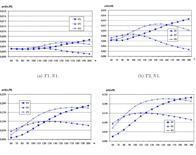
Given the conclusion in Section 2.6, in all our examples we only present results for

the translated gamma approximation obtained with 50 000 simulations for the tables

and 10 000 simulations for the figures. For each Poisson parameter the simulated set

of aggregate claims are the same in each simulation for the three cases of premium

and for the different surpluses. We present for selected cases our estimate of the

ruin probability, ˆψ(u, n), and the standard errors of the estimates for each initial surplus. The time period is 10 years (n = 10). Ten years has been chosen because it is a reasonable planning horizon in practice. The premium in each year is given

(48)

3.3.2 Exponential claim amounts

Consider that the individual claim amounts are exponentially distributed with

mean 1 (variance 1 and skewness 2).

Table 3.8 shows for each of the two target probabilities of ultimate ruin the values

of the parameters A and B to be used in formula (3.19).

target A B

T1 15.38387 ₋1.24137 T2 12.26914 ₋1.22917

Table 3.8: Exponential: Parameters for the power function for formula (3.19).

For the chosen initial surplus, Table 3.9 shows values of the safety loading

ob-tained using De Vylder’s approximation (ζ(uτi, ω)) and given by the fitted power function (AuB

τi). For small initial surpluses in Table 3.9 the fitted formula gives

values for the safety loading higher than the De Vylder’s formula. For higher initial

surpluses the fitted values are lower than De Vylder’s. The ruin probabilities will

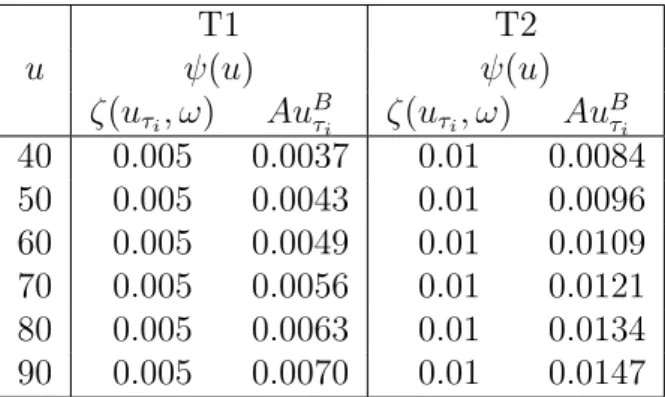
be affected by this as we can see in Table 3.10 for ψ(u) and with more impact in Tables 3.11 to 3.14 forψ(u,10) as we are dealing with finite time.

u T1 T2

ζ(uτi, ω) Au

B

τi ζ(uτi, ω) Au

B

τi

40 0.1481 0.1579 0.1263 0.1317 50 0.1158 0.1197 0.0992 0.1001 60 0.0950 0.0954 0.0816 0.0800 70 0.0806 0.0788 0.0693 0.0662 80 0.0700 0.0668 0.0603 0.0562 90 0.0618 0.0577 0.0533 0.0486

Table 3.9: Exponential: Safety loading obtained by De Vylder’s formula vs fitted power function.

Table 3.10 show the results for the (approximate) probability of ultimate ruin

UNIVERSIDADE TÉCNICA DE LISBOA INSTITUTO SUPERIOR DE ECONOMIA E GESTÃO