B. Klin, P. Soboci´nski (Eds.):
6th Workshop on Structural Operational Semantics (SOS’09) EPTCS 18, 2010, pp. 46–61, doi:10.4204/EPTCS.18.4
c
F. Bonchi, F. Gadducci & G. V. Monreale This work is licensed under the
Creative Commons Attribution License. Filippo Bonchi
Centrum voor Wiskunde en Informatica, Amsterdam, The Netherlands [email protected]
Fabio Gadducci
Dipartimento di Informatica, Universit`a di Pisa, Italy [email protected]
Giacoma Valentina Monreale Dipartimento di Informatica, Universit`a di Pisa, Italy
Reactive systems (RSs) represent a meta-framework aimed at deriving behavioral congruences for those computational formalisms whose operational semantics is provided by reduction rules. RSs proved a flexible specification device, yet so far most of the efforts dealing with their behavioural semantics focused on idem pushouts (IPOs) and saturated (also known as dynamic) bisimulations. In this paper we introduce a novel, intermediate behavioural equivalence: L-bisimilarity, which is able to recast both its IPO and saturated counterparts. The equivalence is parametric with respect to a setLof RSs labels, and it is shown that under mild conditions onLit is indeed a congruence. Furthermore,L-bisimilarity can also recast the notion of barbed semantics for RSs, proposed by the same authors in a previous paper. In order to provide a suitable test-bed, we instantiate our proposal by addressing the semantics of (asynchronous) CCS and of the calculus of mobile ambients.
1
Introduction
Reactive systems(RSs) [12] are an abstract formalism for specifying the dynamics of a computational device. Indeed, the usual specification technique is based on a reduction system, comprising a set of possible states of the device and a relation among them, representing the possible evolutions of the de-vice. The relation is often given inductively, freely instantiating relatively few rewriting rules: despite its ease of use, the main drawback of reduction-based solutions is poor compositionality, since the dynamic behaviour of arbitrary stand-alone terms can be interpreted only by inserting them in appropriate con-texts, where a reduction may take place. The theoretical appeal of RSs is their ability to distill labelled transition systems (LTSs), hence, behavioural equivalences, for devices specified by a reduction system. The idea underlying RSs is simple: whenever a device specified by a termC[P](i.e., a sub-termP
inserted into a unary contextC[−]) may evolve to a stateQ, the associated LTS has a transitionPC−→[−]Q (i.e., the statePevolves intoQwith a labelC[−]). If all contexts are admitted, the resulting semantics is called saturated, and the standard bisimilarity on the derived LTS is a congruence. However, it is unfeasible to check the bisimulation game under all contexts, and usually it suffices to consider a subset of contexts that guarantees that the distilled behavioural semantics is a congruence. Such a set, the “minimal” contexts allowing a reduction to occur, was identified in [12] by the notion ofrelative pushout: the resulting strong bisimilarity is a congruence, even if it often does not coincide with the saturated one. Several attempts have been made to encode various specification formalisms (Petri nets [15, 20], logic programming [6], etc.) as RSs, either hoping to recover the standard observational equivalences, whenever such a behavioural semantics exists (CCS [13], pi-calculus [14], etc.), or trying to distill a
∗Research partly supported by the EU within the FP6-IST IP 16004 SENSORIA(Software Engineering for Service-Oriented
meaningful new semantics. The results are often not fully satisfactory: bisimilarity via minimal con-texts is usually too fine-grained; while saturated semantics are often too coarse (the standard CCS strong bisimilarity is e.g. strictly included in the saturated one). As for process calculi, the standard way out of the empasse it to considerbarbs[16] (i.e., predicates on the states of a system) and barbed equivalences (i.e., adding the check of such predicates in the bisimulation game). The flexibility of the definition allows for recasting a variety of observational, bisimulation-based equivalences. Indeed, the method-ological contribution of [5] is the introduction of suitable notions of barbed saturated semantics for RSs. In this paper we move one step further, and we propose a novel behavioural equivalence for RSs, namely,L-bisimulation: a flexible tool, parametric with respect to a set of minimal labelsL. Also in this case the idea is very simple, and it just asymmetrically refines the standard bisimulation game. If the
minimal LTS has a transitionPC−→[−]Q, then a bisimilarP′has to react via a minimal transitionP′C−→[−]Q′, wheneverC[−]∈L; or it must ensure thatC[P′]may evolve intoQ′ (thus requiring no minimality for C[−]with respect to P′), otherwise. The associated bisimilarity is intermediate between the standard semantics (i.e., minimal and saturated) for RSs: indeed, it is able to recover both of them, by simply varying the setLand exploiting the so-called semi-saturated semantics. It can be proved that, under mild closure conditions on the setL,L-bisimilarity is a congruence; and moreover, it can be shown that barbed saturated semantics can be recast, as long asLsatisfies suitable barb-capturing properties.
With respect to barbed saturated semantics, L-bisimilarity admits a streamlined definition, where state predicates play no role. It is thus of simpler verification, and its introduction may have far reaching consequences over the usability of the RS formalism. However, as for any newly proposed semantics, its adequacy and ease of use have to be tested against suitable case studies. We thus consider a recently introduced, minimal context semantics for mobile ambients (MAs), as distilled in [4]; as well as two min-imally labelled transition systems for CCS and its asynchronous variant, reminiscent of those proposed in [3]. We show that in those cases, a setLof minimal labels can be identified, such thatL-bisimilarity precisely captures the standard semantics of the calculus at hand.
The paper is organized as follows. Section 2 recalls the basic notions of RSs, while Section 3 and Section 4 perform the same for MAs and (asynchronous) CCS, respectively. Section 5 presents the tech-nical core of the paper: the introduction ofL-bisimilarity for RSs, the proof that (under mild conditions onL) it is indeed a congruence, and moreover its correspondence with barbed semantics. Finally, Sec-tion 6 and SecSec-tion 7 prove that, suitably varying the setL, the newly definedL-bisimilarity captures the standard equivalences for MAs and for CCS and its asynchronous variant, respectively.
2
Reactive Systems
This section summarizes the main results concerning (the theory of) reactive systems (RSs) [12]. The formalism aims at deriving labelled transition systems (LTSs) and bisimulation congruences for a system specified by a reduction semantics, and it is centered on the concepts ofterm,contextandreduction rule: contexts are arrows of a category, terms are arrows having as domain 0, a special object that denotes groundness, and reduction rules are pairs of (ground) terms.
Definition 1(Reactive System). Areactive systemCconsists of
1. a categoryC;
2. a distinguished object0∈ |C|;
3. a composition-reflecting subcategoryDof reactive contexts; 4. a set of pairsR⊆S
I4
I2
C[−] @@
I3 d ^ ^ >>> 0 P _ _ ???? l ? ? I4 I2
C[−] @@
e//I5
gOO
I3 f o o d ^ ^ >>> 0 P _ _ ???? l ? ? I6 I2
e′ @@
e //I5
hOO
I3 f o o f′ ^ ^
>>> I4
I6
g′ @@
I5 g O O h o o
(i) (ii) (iii) (iv)
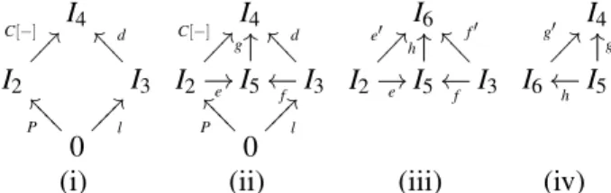
Figure 1: Redex Square and RPO
Intuitively, reactive contexts are those in which a reduction may occur. By composition-reflecting we mean thatd′◦d∈Dimpliesd,d′∈D. Note that the rules have to be ground, i.e., left-hand and right-hand sides have to be terms without holes and, moreover, with the same codomain.
The reduction relation is generated from the reduction rules by closing them under all reactive con-texts. Formally, thereduction relationis defined by takingP Qif there ishl,ri ∈Randd∈Dsuch
thatP=d◦landQ=d◦r.
Thus the behaviour of an RS is expressed as an unlabelled transition system. In order to obtain a LTS, we can plug a termP into some contextC[−]and observe if a reduction occurs. In this case we
have thatPC−→[−]. Categorically speaking, this means thatC[−]◦Pmatchesd◦lfor some rulehl,ri ∈R
and some reactive contextd. This situation is formally depicted by diagram (i) in Fig. 1: a commuting diagram like this is called aredex square.
Definition 2(Saturated Transition System). Thesaturated transition system(STS) is defined as follows
• states: arrows P: 0→I inC, for arbitrary I;
• transitions: P→C[−]SAT Q if C[P] Q.
Note thatC[P]stands forC[−]◦P: the same notation is used in Definitions 3 and 7 below, in order to allow for an easier comparison with the process calculi notation, to be adopted in the following sections.
Definition 3(Saturated Bisimulation). A symmetric relationR is asaturated bisimulationif whenever
PRQ then∀C[−]
• if C[P] P′then C[Q] Q′and P′RQ′.
Saturated bisimilarity∼Sis the largest saturated bisimulation.
It is obvious that ∼S is a congruence. Indeed, it is the coarsest symmetric relation satisfying the bisimulation game on that is also a congruence.
Note that STS is often infinite-branching since all contexts allowing reductions may occur as labels. Moreover, it has intuitively redundant transitions. For example, consider the terma.0 of CCS. We have
both the transitionsa.0→a.0|−SAT 0|0 anda.0 P|a.0|−
→SAT P|0|0, yetPdoes not “concur” to the reduction. We thus need a notion of “minimal context allowing a reduction”, captured byidem pushouts.
Definition 4(RPO, IPO). Let the diagrams in Fig. 1 be in a category C, and let (i) be a commuting diagram. Acandidatefor (i) is any tuplehI5,e,f,gimaking (ii) commute. A relative pushout (RPO)is
the smallest such candidate, i.e., such that for any other candidatehI6,e′,f′,g′i there exists a unique
morphism h:I5→I6making (iii) and (iv) commute. A commuting square such as diagram (i) of Fig. 1 is
calledidem pushout (IPO)ifhI4,c,d,idI4iis its RPO.
Definition 5(IPO Transition System). TheIPO transition system(ITS) is defined as follows
• states: P: 0→I inC, for arbitrary I;
• transitions: P→C[−]IPOd◦r if d∈D,hl,ri ∈R, and (i) in Fig. 1 is an IPO.
In other words, if insertingP into the contextC[−]matchesd◦l, andC[−]is the “smallest” such context, thenPevolves tod◦rwith labelC[−].
Bisimilarity on ITS is referred to asIPO-bisimilarity(∼I). Leifer and Milner have shown that if the RS has redex RPOs, then it is a congruence.
Proposition 1. Let us consider an RS with redex RPOs. Then,∼Iis a congruence.
Clearly, ∼I⊆∼S. In [2] the first author shows that this inclusion is strict for many formalisms. In particular, it turns out that in some interesting cases∼I is too strict, while∼S is too coarse. This fact is the reason for introducingbarbed bisimilarities[16]. Barbs are predicates (representing some basic observations) on the states of a system. For instance, in [16] the authors use for CCS barbs↓a and↓a¯
representing the ability of a process to perform an input, respectively an output, on channela. In the following we fix a familyOof barbs, and we writeP↓oifPsatisfieso∈O.
Definition 6(Barbed Saturated Bisimulation). A symmetric relationRis abarbed saturated bisimulation
if whenever PRQ then∀C[−]
• if C[P]↓othen C[Q]↓o;
• if C[P] P′then C[Q] Q′and P′RQ′.
Barbed saturated bisimilarity∼BSis the largest barbed saturated bisimulation.
It is easy to see that∼BSis the largest barbed bisimulation that is also a congruence.
2.1 An Efficient Characterization of (Barbed) Saturated Bisimilarity
Since the definition of saturated bisimulation involves a quantification over all possible contexts, it is usually hard to (automatically) prove the equivalence of two systems. For this reason, the first author, with K¨onig and Montanari, introducedsemi-saturated bisimilarity[6].
Definition 7(Semi-Saturated Bisimulation). A symmetric relationRis asemi-saturated bisimulationif
whenever PRQ then
• if P→C[−]IPOP′then C[Q] Q′and P′RQ′.
Semi-saturated bisimilarity∼SSis the largest barbed semi-saturated bisimulation.
Proposition 2. Let us consider an RS with redex IPOs. Then,∼SS=∼S.
Reasoning on∼SS is easier than on∼S because instead of looking at the reductions in all contexts, only IPO transitions are considered.
In [5], the authors extended this technique to barbed saturated bisimilarity.
Definition 8(Barbed Semi-Saturated Bisimulation). A symmetric relationRis abarbed semi-saturated
bisimulationif whenever PRQ then
• ∀C[−], if C[P]↓othen C[Q]↓o;
• if P→C[−]IPOP′then C[Q] Q′and P′RQ′.
Proposition 3. Let us consider an RS with redex IPOs. Then,∼BSS=∼BS.
Also in this case, it is more convenient to work with∼BSS instead of ∼BS. Even if barbs are still quantified over all contexts, for many formalisms (as for MAs) it is actually enough to check if P↓o implies Q↓o, since this condition implies that ∀C[−], ifC[P]↓o thenC[Q]↓o. Barbs satisfying this property are calledcontextualbarbs.
Definition 9(Contextual Barbs). A barb o is acontextual barbif whenever P↓oimplies Q↓othen∀C[−], C[P]↓oimplies C[Q]↓o.
3
Mobile Ambients
In this section we first introduce the finite, communication-free fragment of mobile ambients (MAs) [8] and its reduction semantics. Then, we recall the IPO transition system for MAs presented in [4].
Fig. 2 shows the syntax of the calculus. We assume a set N ofnamesranged over by m,n,u, . . ..
Besides the standard constructors, we include a set{X,Y, . . .}ofprocess variables and a set{x,y, . . .}
ofname variables. We letP,Q,R, . . .range over the set ofpure processes, containing neither process nor name variables; whilePε,Qε,Rε, . . .range over the set of well-formedprocesses, i.e., such that no
process or ambient variable occurs twice.
Intuitively, an impure process such as x[P]|X represents an underspecified system, where either the processX or the name of the ambientx[−]can be further instantiated. These extended processes are needed later for the presentation of the LTS. We use the standard definitions for the set of free names of a pure processP, denoted by f n(P), and forα-convertibility, with respect to the restriction operators(νn).
We moreover assume that f n(X) = /0 and f n(x[P]) = f n(P). We also consider a family ofsubstitutions, which may replace a process/name variable with a pure process/name, respectively. Substitutions avoid name capture: for a pure processP, the expression (νn)(νm)(X|x[0]){m/
x,n[P]/X}corresponds to the pure process(νp)(νq)(n[P]|m[0]), for names p,q6∈ {m} ∪f n(n[P]).
The semantics of the calculus exploits a structural congruence, denoted by ≡, which is the least equivalence on pure processes that satisfies the axioms in Fig. 3. Thereduction relation, denoted by , describes the evolution of pure processes. It is the smallest relation closed under the congruence≡and inductively generated by the set of axioms and inference rules in Fig. 4.
As already said, abarb ois a predicate over the states of a system, withP↓odenoting thatPsatisfies o. In MAs, P↓n denotes the presence at top-level of an unrestricted ambientn. Formally, for a pure processP,P↓nifP≡(νA)(n[Q]|R)andn6∈A, for processesQandRand a set of restricted namesA.
Definition 10(Reduction Barbed Congruences [18]). Reduction barbed congruence∼MAis the largest symmetric relationR such that whenever PRQ then
• if P↓nthen Q↓n;
• if P P′then Q Q′and P′RQ′;
• ∀C[−],C[P]RC[Q].
P::=0,n[P],M.P,(νn)P,P1|P2,X,x[P] M::=in n,out n,open n
Figure 2: (Extended) Syntax of mobile ambients.
ifP≡QthenP|R≡Q|R P|0≡P
ifP≡Qthen(νn)P≡(νn)Q (νn)(νm)P≡(νm)(νn)P
ifP≡Qthenn[P]≡n[Q] (νn)(P|Q)≡P|(νn)Q ifn∈/ f n(P)
ifP≡QthenM.P≡M.Q (νn)m[P]≡m[(νn)P] ifn6=m P|Q≡Q|P (νn)M.P≡M.(νn)P ifn∈/ f n(M) (P|Q)|R≡P|(Q|R) (νn)P≡(νm)(P{m/
n}) ifm∈/ f n(P)
Figure 3: Structural congruence.
n[in m.P|Q]|m[R] m[n[P|Q]|R] ifP Qthen(νn)P (νn)Q m[n[out m.P|Q]|R] n[P|Q]|m[R] ifP Qthenn[P] n[Q]
open n.P|n[Q] P|Q ifP QthenP|R Q|R
Figure 4: Reduction relation on pure processes.
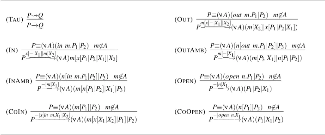
An ITS for Mobile Ambients. Here we present the ITSM for MAs proposed in [4]. The inference rules describing this LTS are obtained from an analysis of a LTS over (processes as) graphs, derived by the borrowed context mechanism [10], which is an instance of the theory of RSs [21]. The labels of the transitions are unary contexts, i.e., terms of the extended syntax with a hole−. Note that they are minimal contexts, that is, they represent the exact amount of context needed by a system to react. We denote them byCε[−]. The formal definition of the LTS is presented in Fig. 5.
The rule TAUrepresents theτ-actions modeling internal computations. Notice that the labels of the
transitions are identity contexts composed of just a hole−, while the resulting states are pure processes. The other rules in Fig. 5 model the interactions of a process with its environment. Note that both labels and resulting states contain process and name variables. We define the LTSMIfor processes over the standard syntax of MAs by instantiating all the variables of the labels and of the resulting states.
Definition 11. Let P,Q be pure processes and let C[−]be a pure context. Then, we have that PC−→[−]MIQ
if there exists a transition PCε[−]
−−→MQε and a substitutionσ such that Qεσ≡Q and Cε[−]σ=C[−].
In the above definition recall that substitutions replace process variables by pure processes and that they do not capture bound names.
The rule OPEN models the opening of an ambient provided by the environment. In particular, it enables a process P with a capability open n at top level, for n ∈ f n(P), to interact with a context providing an ambientn containing some processX1. Note that the label−|n[X1]of the rule represents
the minimal context needed by the processP for reacting. The resulting state is the process over the extended syntax(νA)(P1|X1|P2), whereX1represents a process provided by the environment. Note that
the instantiation of the process variableX1 with a process containing a free name that belongs to the
bound names inAis possible onlyα-converting the resulting process(νA)(P1|X1|P2)into a process that
does not contain that name among its bound names at top level.
(TAU) P Q
P−→−Q (OUT)
P≡(νA)(out m.P1|P2) m6∈A
Pm[x[−−−−−−|X1]|X→(2]νA)(m[X2]|x[P1|P2|X1])
(IN) P≡(νA)(in m.P1|P2) m6∈A
Px[−−−−−−|X1]|m[X→(2]νA)m[x[P1|P2|X1]|X2]
(OUTAMB) P≡(νA)(n[out m.P1|P2]|P3) m6∈A
Pm[−−−|X→(1]νA)(m[P3|X1]|n[P1|P2])
(INAMB) P≡(νA)(n[in m.P1|P2]|P3) m6∈A
P−|−−m[X→(1]νA)(m[n[P1|P2]|X1]|P3)
(OPEN) P≡(νA)(open n.P1|P2) n6∈A
P−|−−n[X→(1]νA)(P1|P2|X1)
(COIN) P≡(νA)(m[P1]|P2) m6∈A
P−|−−−−−−x[in m.X1|X→(2]νA)(m[x[X1|X2]|P1]|P2)
(COOPEN) P≡(νA)(n[P1]|P2) n6∈A
P−|−−−−open n.→(X1 νA)(P1|X1|P2)
Figure 5: The LTSM.
while in the rule IN both ambients are provided by the environment. In the rule COIN an ambient provided by the environment enters an ambient of the process. The rule OUTAMBmodels an ambient of the process exiting from an ambient provided by the environment, while in the rule OUT both ambients are provided by the environment.
4
On Synchronous and Asynchronous CCS
This section introduces the ITSs for CCS and for its asynchronous variant. For the sake of space, we do not present the standard CCS, while we indeed recall the syntax and the semantics of Asynchronous CCS (ACCS). We then show an ITS for both CCS and ACCS: the former was introduced in [3], while the latter is original. Finally, we show that the IPO-bisimilarity coincides with the ordinary bisimilarity for CCS; while IPO-bisimilarity is strictly contained in asynchronous bisimilarity.
Asynchronous CCS. Differently from synchronous calculi, where messages are simultaneously sent and received, in asynchronous communication the messages are sent and travel through some media until they reach destination. Thus sending is non blocking (i.e., a process may send even if the receiver is not ready to receive), while receiving is (processes must wait until a message becomes available). Observations reflect the asymmetry: since sending is non blocking, receiving is unobservable.
Here we shortly introduce the finite fragment of ACCS. We adopt a presentation reminiscent of asynchronousπ[1] that allows the non deterministic choice for input prefixes (a feature missing in [7, 9]).
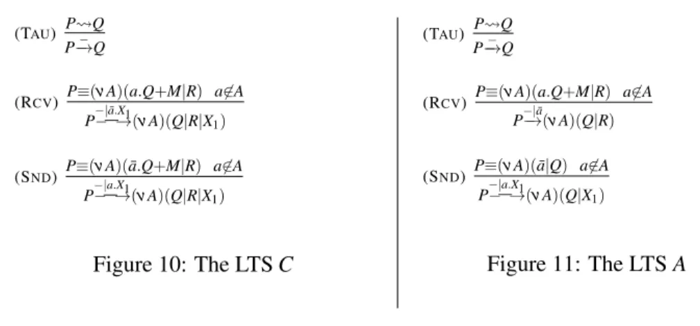
Fig. 6 shows the syntax of the calculus. We assume a setN ofnamesranged over bya,b,c, . . .. As
for MAs, we included a set{X,Y, . . .}ofprocess variables. These are needed for the presentation of the LTS in Fig. 11. We letP,Q,R, . . .range over the set ofpureprocesses, containing no process variables. Substitution of process variables is defined analogously to MAs. Note that here we letM,N,O, . . .range over the set of summation, while in MAs we used those symbols for capabilities.
P::=M,X, a¯, (νa)P, P1|P2 M::=0, τ.P, a.P, M1+M2
Figure 6: (Extended) Syntax of Asynchronous CCS.
ifP≡QthenP|R≡Q|R P|0≡P
ifP≡Qthen(νa)P≡(νa)Q (νa)(νb)P≡(νb)(νa)P
ifP≡Qthenτ.P≡τ.Q (νa)(P|Q)≡P|(νa)Q ifa∈/ f n(P)
ifP≡Qthena.P≡a.Q M+N≡N+M
ifM≡NthenM+O≡N+O (M+N) +O≡M+ (N+O)
P|Q≡Q|P M+0≡M
(P|Q)|R≡P|(Q|R) (νa)P≡(νb)(P{b/
a}) ifb∈/ f n(P)
Figure 7: Structural congruence.
(a.P+M)|a¯ P ifP Qthen(νa)P (νa)Q
τ.P+M P ifP QthenP|R Q|R
Figure 8: Reduction relation on pure processes.
a.P+M−→a P ifP−→µ Qthen(νa)P−→µ (νa)Q ifa∈/n(µ)
τ.P+M−→τ P ifP−→µ QthenP|R−→µ Q|R
¯
a−→a¯ 0 ifP−→a P1andQ ¯
a
−→Q1thenP|Q
τ −→P1|Q1
Figure 9: Labelled transition system.
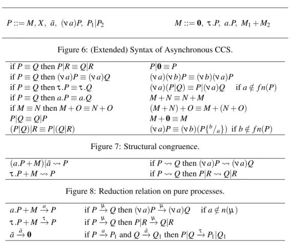
Structural equivalence(≡) is the smallest congruence induced by the axioms in Fig. 7. The behaviour of a processPis then described as a reaction relation ( ) over processes up to≡, obtained by closing the rules in Fig. 8. For ACCS, there exists also an interactive semantics expressed by an LTS. This is the transition relation over processes up to≡, obtained by the rules in Fig. 9. Here we use µ to range over
the set of labels{τ,a,a¯|a∈N }. The names ofµ, denoted byn(µ), are defined as usual.
The main difference with respect to the synchronous calculus lies in the notion ofobservation. Since sending messages is non-blocking, an external observer can just send messages to a system without knowing if they will be received or not. For this reason receiving should not be observable and thus barbs take into account only outputs. Formally,P↓a¯if there exists processQsuch thatP−→a¯ Q. This is reflected in the notion of asynchronous bisimilarity [1].
Definition 12(Asynchronous Bisimulation). A symmetric relationRis anasynchronous bisimulationif
whenever PRQ then
• if P−→τ P′ then Q−→τ Q′and P′RQ′,
• if P−→a¯ P′ then Q−→a¯ Q′and P′RQ′,
• if P−→a P′ then either Q−→a Q′and P′RQ′or Q−→τ Q′and P′RQ′|a.¯
Asynchronous bisimilarity∼Ais the largest asynchronous bisimulation.
(TAU) P Q
P−→−Q
(RCV) P≡(νA)(a.Q+M|R) a6∈A
P−|−−a¯.→(X1 νA)(Q|R|X1)
(SND) P≡(νA)(a.Q¯ +M|R) a6∈A
P−|−−a.→(X1 νA)(Q|R|X1)
Figure 10: The LTSC
(TAU) P Q
P−→−Q
(RCV) P≡(νA)(a.Q+M|R) a6∈A
P−|−→(a¯νA)(Q|R)
(SND) P≡(νA)(a¯|Q) a6∈A
P−−|−a.→(X1 νA)(Q|X1)
Figure 11: The LTSA
An ITS for CCS. In [3], the first and the second author together with K¨onig derived an ITS for the ordinary CCS by employing the borrowed context mechanism [10].
Fig. 10 shows the LTSC. The labels ofCare minimal contexts, i.e., they represent the exact amount of context needed by a process to react. The reactive semantics of CCS (denoted by ) can be found in [14]. Note that both the labels and the resulting states contain the process variableX1. For the sake of
space, we avoided to report here the (extended) syntax of CCS: this is just the ordinary syntax of CCS, together with process variables (analogously to MAs and ACCS).
Following Definition 11 for MAs, we define the LTSCI for processes over the standard syntax by instantiating the process variable of the labels and of the resulting states.
Now let us consider the rule RCV. If a process is ready to receive on some unrestricted channela, then an interaction takes place whenever it is embedded in an environment of the shape−|a¯.X11. Recall
that the instantiation of the process variableX1with a process containing a free name that belongs to the
bound names inAis possible onlyα-converting the resulting process(νA)(Q|R|X1).
Hereafter we use −→µ (with µ ∈ {τ,a,a¯|a∈N }) to denote the ordinary LTS of CCS [13]. By
comparing the latter with the LTSC, it is easy to see thatP−→τ Qif and only ifP−→− Q. MoreoverP−→a Q iffP−|−−→a.X¯ 1Q|X1andP−→a¯ QiffP
−|a.X1
−−→Q|X1. From these facts, the main result of [3] follows: the ordinary
bisimilarity of CCS (denoted by∼CCS) coincides with IPO bisimilarity. Instead, saturated bisimilarity is too coarse: the (recursive) processesP=reczτ.zandP|a.0are e.g. saturated bisimilar.
An ITS for ACCS. Following [3], we propose an ITS for ACCS. Fig. 11 shows the LTSA. The LTS AIis defined by instantiating the process variable of the labels and of the resulting states.
The main difference between A andC is in the rule RCV: since outputs have no continuation in ACCS, then the process variableX1(that occurs inC) is not needed inA.
It is easy to see that also for ACCS there is a close correspondence between the ordinary LTS
seman-tics (in Fig. 9) andA:P−→τ QiffP−→− Q,P−→a QiffP−−|→a¯QandP−→a¯ QiffP−|−−→a.X1Q|X1.
However, in the asynchronous case, IPO-bisimilarity is too fine grained. Indeed, the processesa.a¯+ τ.0 andτ.0 are asynchronously bisimilar, but they are not IPO-bisimilar. In the next section we will
introduce a new semantics for RSs that generalizes both∼CCSand∼A.
5
A New Semantics for Reactive Systems:
L
-Bisimilarity
As shown in Section 4, IPO-bisimilarity coincides with the ordinary bisimilarity in the case of CCS. However, for many interesting calculi, such as MAs and ACCS, it is often too fine-grained. On the other side, as recalled above for CCS, saturated bisimilarity is often too coarse.
In this section we introduceL-indexed bisimilarity (shortly,L-bisimilarity), a novel kind of bisimilar-ity parametric with respect to a class of contexts (also referred to aslabels)L. For each classLsatisfying some closure properties, the new equivalence∼Lis a congruence and∼I⊆∼L⊆∼S.
Intuitively,L-bisimulations can be thought of as something in between IPO-bisimulations and
semi-saturated bisimulations: ifC[−]belongs toL, thenQmust performQ→C[−]IPOwheneverP C[−]
→IPO(as in the IPO-bisimulation), otherwiseC[Q] (as in the semi-saturated bisimulation).
Definition 13(L-Bisimulation). Let L be a class of contexts. A symmetric relationRis an L-bisimulation
if whenever PRQ then
if P→C[−]IPOP′then
(
Q→C[−]IPOQ′and P′RQ′, if C[−]∈L; C[Q] Q′and P′RQ′, otherwise.
L-bisimilarity∼Lis the largest L-bisimulation.
It is easy to note that∼Lgeneralizes both∼Iand∼SS(and thus∼S). Indeed, in order to characterize the former, it is enough to take asLthe whole class of contexts, while to characterize the latter, we take asLthe empty class. In Section 5.1 we will show that for some L, L-bisimilarity also coincides with barbed saturated bisimilarity. In the remainder of this section, we show that∼Lis a congruence. In order to prove this, we have to require the following condition onL.
Definition 14. Let L be a class of arrows of a category. We say that L is IPO-closed, if whenever the following diagram is an IPO and b∈L, then also c∈L.
b ?? d _ _ ???? ? a _ _ ?? ??? c??
It is often hard to prove that a class of contexts is IPO-closed. It becomes easier with concrete instances of RSs that supply a constructive definition for IPOs, such as bigraphs and borrowed contexts.
Proposition 4. Let us consider a RS with redex RPOs and an IPO-closed class L of contexts. Then,∼L is a congruence.
k6
k4
J[−] ?? k2 C[−] _ _ ?? ??? k3 D[−] ^ ^ == == == == == === 0 P ^ ^ >>
>>> L@@
k6
k4
J[−] ??
k5
D2[−]
_ _ ?? ??? k2 C[−] _ _ ?? ???J
′[−] ?? k3
D1[−]
_ _ ?? ??? 0 P ` ` @@
@@@ ~~L~?? ~ ~
k6
k4
J[−] ??
k5
D2[−]
_ _ ?? ??? k2 C[−] _ _ ?? ???J
′[−] ?? k3 E[−] _ _ ?? ??? 0 Q ` ` @@ @@@ L′ ? ? ~ ~ ~ ~ ~
Proof. In order to prove this theorem we will use the composition and decomposition properties of IPOs, namely Proposition 2.1 and Proposition 2.2 of [12]. We have to prove that ifP∼LQthenC[P]∼LC[Q]. We show thatR={(C[P],C[Q])s.t.P∼LQ}is anL-bisimulation.
Suppose thatC[P]→J[−]IPOP′. Then there exists an IPO square like diagram (i) above, wherehL,Ri ∈R, D[−]∈DandP′=D[R]. Since, by hypothesis, the RS has redex RPOs, then we can construct an RPO as the one in diagram (ii) above. In this diagram, the lower square is an IPO, since RPOs are also IPOs (Proposition 1 of [12]). Since the outer square is an IPO and the lower square is an IPO, by IPO decomposition property, it follows that also the upper square is an IPO.
SinceDis composition-reflecting, then bothD1[−]andD2[−]belong toD, and thenP J
′[−]
→IPOD1[R]. Now there are two cases: eitherJ[−]∈LorJ[−]∈/L.
IfJ[−]∈L, then alsoJ′[−]∈L, becauseLis IPO-closed, by hypothesis. SinceP∼LQ, thenQ→J′[−] IPO Q′′andD1[R]∼LQ′′. This means that there exists an IPO square like the lower square of diagram (iii)
above, wherehL′,R′i ∈R, E[−]∈DandE[R] =Q′′. Now recall by the previous observation that the
upper square of diagram (iii) is also an IPO and then, by IPO composition, also the outer square is an
IPO. This means thatC[Q]→J[−]IPOD2[Q′′]. SinceD1[R]∼LQ′′, thenP′=D[R] =D2[D1[R]]RD2[Q′′].
If J[−]∈/L, then either J′[−]∈L orJ′[−]∈/ L. In both cases, from P J
′[−]
→IPOD1[R]we derive that J′[Q] Q′′andD1[R]∼LQ′′. This means that the lower square of diagram (iii) above commutes. Since
also the upper square commutes, then also the outer square commutes. This means thatC[Q] D2[Q′′].
SinceD1[R]∼LQ′′, thenP′=D[R] =D2[D1[R]]RD2[Q′′].
5.1 Barbed Saturated Bisimilarity viaL-bisimilarity
Here we show thatL-bisimilarity can also characterize barbed saturated bisimilarity, whenever the family of barbs and the set of labelsLsatisfy suitable conditions. This result will be used in later sections in order to show thatL-bisimilarity captures the correct equivalences for MAs and ACCS.
In order to guarantee that∼L⊆∼BS, we need some conditions ensuring that the checking of barbs of
∼BSis already done in∼Lby the labels inL.
Definition 15. Let L be a set of labels and let O be a set of barbs. We say that L is O-capturingif for
each barb o there exists a label C[−]∈L such that for each process P, P↓oif and only if P C[−]
→IPOP′.
The next two definitions are needed to ensure that∼BS⊆∼L.
Definition 16. LetR be a relation and letP(X,Y)be a predicate on processes. We say thatP(X,Y)
isstable underRif whenever PRQ andP(P,P′)there exists Q′such thatP(Q,Q′)and P′RQ′.
For example, the predicates in Fig. 12 and Fig. 13 are stable under∼BS.
Definition 17. LetR be a relation and let C[−]be a label. We say that C[−]isstable under R if the
predicateP(X,Y) =X→C[−]IPOY is stable underR.
We can finally state a first correspondence result.
Proposition 5. Let us consider an RS with redex RPOs, a set O of contextual barbs and a set L of labels. If L is O-capturing and its labels are stable under∼BS, then∼BS coincides with∼L.
Suppose thatP→C[−]IPOP′. We have two cases: eitherC[−]∈LorC[−]∈/L. IfC[−]∈L, thenC[−]
is stable under∼BSand thus, sinceP∼BSQ,Q→C[−]
IPOQ′andP′∼BSQ′. For the case thatC[−]∈/L, it is enough to note that, sinceP→C[−]IPOP′, thenC[P] P′. SinceP∼BSQ, thenC[Q] Q′andP′∼BSQ′.
Now we show thatR={(P,Q)s.t.P∼LQ}is a barbed semi-saturated bisimulation (i.e.,∼L⊆∼BSS) and thus, since the RS has redex IPOs, by Proposition 3 it follows that∼L⊆∼BS.
At first, we note that, sinceOis a set of contextual barbs, in order to show thatRsatisfies the first
condition of Definition 8 it suffices to show thatP↓oimpliesQ↓o. SinceLisO-capturing, ifP↓othen there is a labelC[−]∈Lsuch thatP↓oif and only ifP
C[−]
→IPO. SinceP∼LQ, then alsoQ C[−]
→IPOandQ↓o.
In order to prove the second condition of Definition 8, it is enough to note that ifP→C[−]IPOP′then, for eitherC[−]∈LorC[−]∈/L,C[Q] Q′withP′∼LQ′.
As a corollary of the previous definition, we obtain the following property that allows to check whenever IPO-bisimilarity coincides with barbed saturated one.
Lemma 1. Let us consider an RS with redex IPOs and a set O of contextual barbs. If the set of all labels is O-capturing and each label is stable under∼BS, then∼I coincides with∼BS.
6
L
-Bisimilarity for Mobile Ambients
This section proposes a new labelled characterization of the reduction barbed congruence for MAs, presented in Section 3. In particular, by using the ITSMI (also in Section 3) we define anL-bisimilarity that captures barbed saturated bisimilarity for MAs, coinciding with reduction barbed congruence.
Proposition 6(see [5], Theorem 3). Reduction barbed congruence over MAs∼MAcoincides with barbed saturated bisimilarity∼BS
M .
As shown in Section 5.1, we can characterize barbed saturated bisimilarity on a set of contextual barbsOthrough the IPO transition system and a set of labelsL. In particular, as required by Proposition 5, the setLmust beO-capturing and eachC[−]∈Lmust be stable under the barbed saturated bisimilarity.
We denote byOMthe set of barbs of MAs, recalling that MAs barbs are contextual barbs [5].
Proposition 7(see [5], Proposition 6). OM is a set of contextual barbs.
Therefore, we can characterize reduction barbed congruence over MAs by instantiating Defini-tions 13 with the ITSMIand a setLof labels having the two properties said above.
First of all, we find some labels ofMI that capture the barbs of MAs. This ensures that the checking of barbs of the barbed saturated bisimilarity is done in the L-bisimilarity by the first condition of its definition. It is easy to note that a MAs processP observes a unrestricted ambient n at top-level, in symbolsP↓n, if and only if it can execute a transition labelled with−|open n.T1or with−|m[in n.T1|T2].
Therefore,LisOM-capturing if it contains at least one kind of these labels. We choose to consider labels of the first type, that is, having the shape−|open n.T1, fornambient name andT1pure process.
It is possible to prove that these labels are stable under ∼BS
M . Therefore, if we consider the set L defined below, we obtain anL-bisimilarity for MAs that is able to characterize∼BS
M .
Proposition 8. Let LMbe the set of all labels of theITSMIhaving the shape−|open n.T1, for n ambient
P−|open n.T1(X,Y) ∃P′′andm6∈ f n(X)s.t. P′′↓
m,C′[X] P′′ Y andY 6↓m withC′[−] =−|open n.(m[0]|open m.T1)
Figure 12: Predicate for the label−|open n.T1.
Proof. We have to show that for each barbn∈OM there exists a labelC[−]∈LM such that for each
processP,P↓nif and only ifP C[−]
−→MIP
′.
It is easy to note that, given a barb n∈OM, we have that for each process P, P↓n if and only if P−|−−−−−→open n.T1MI P
′, with T
1 pure process. Since we know that LM contains all labels having the shape
−|open n.T1, fornambient name andT1pure process, we can conclude thatLM isOM-capturing.
Now, in order to prove that eachC[−]∈LMis stable under∼BSM , we exploit a predicate such that it is stable under∼BS
M and equivalent to the one of Definition 17.
Lemma 2. LetP−|open n.T1(X,Y)be the binary predicate on MAs processes shown in Fig. 12, for n
ambient name and T1pure process. Then,P−|open n.T1(X,Y)is stable under∼BSM and for each P and P
′,
P−|open n.T1(P,P′)if and only if P−|−−−−−→open n.T1
MIP
′.
Proof. We begin by proving that the predicateP−|open n.T1(X,Y)is stable under∼BS
M .
Assume thatP∼BS
M QandP
−|open n.T1(P,P′)holds. SinceP−|open n.T1(P,P′)holds, then there exists
a processP′′and an ambientmfresh forPandQ, such thatC′[P] P′′,P′′↓m,P′′ P′andP′6↓m, with C′[−] =−|open n.(m[0]|open m.T1).
Since C′[P] P′′ and P∼BS
M Q, then C′[Q] Q′′ and P′′∼ BS
M Q′′. Therefore, it is obvious that also Q′′↓m. Now, we know thatP′′ P′, hence we can say thatQ′′ Q′ andP′∼BSM Q
′. From this
follows that, since P′6↓m, then alsoQ′6↓m. So, we can conclude that P−|open n.T1(Q,Q′) holds, hence P−|open n.T1(X,Y)is stable underR.
Now we show that for eachPandP′,P−|open n.T1(P,P′)iffP−|−−−−−→open n.T1
MIP
′.
Assume thatP−|open n.T1(P,P′)holds. This means that there exists a processP′′and an ambientm
fresh forP, such thatC′[P] P′′,P′′↓m,P′′ P′andP′6↓m, withC′[−] =−|open n.(m[0]|open m.T1). The fact thatC′[P] P′′andP′′↓mmeans that the capabilityopen nhas been executed, hence there must be a unrestricted ambientnat top-level ofP, i.e.,P≡(νA)(n[P1]|P2)andn6∈A. From this follows that P′′= (νA)(P1|P2)|m[0]|open m.T1, and since P′6↓m, thenP′ ≡(νA)(P1|P2)|T1. Moreover, by knowing
thatP= (νA)(n[P1]|P2)andn6∈A, we can conclude thatP−|−−−−−→open n.T1MIP
′.
Assume that P−|−−−−−→open n.T1P′. This means that P≡Q, where Q= (νA)(n[P1]|P2), n6∈Aand P′= (νA)(P1|P2)|T1. We consider the contextC′[−] =−|open n.(m[0]|open m.T1)withm6∈ f n(P). It is easy
to note thatC′[Q] P′′s.t.P′′= (νA)(P1|P2)|m[0]|open m.T1andP′′↓m. Therefore, sinceC′[P]≡C′[Q],
we also have thatC′[P] P′′. Now, we can note thatP′′ P′and, sincemis fresh forP,P′6↓m.
Proposition 9. All labels in LMare stable under∼BSM .
The proof of the proposition above trivially follows from Lemma 2. We finally introduce the main characterization proposition.
Proposition 10. ∼BS
M =∼
Proof. First of all, by Proposition 7, we know that MAs barbs are contextual. Moreover, by Propositions 8 and 9, we know thatLisOM-capturing and it contains only labels that are stable under∼BSM . Therefore, thanks to Proposition 5, we can conclude that∼BS
M =∼
LM.
The L-bisimilarity ∼LM presented above is not the only one which is able to characterize barbed saturated bisimilarity ∼BS
M . For example, as said before, we can choose to consider all labels of the shape−|m[in n.T1|T2]: besides being able to capture MAs barbs, they are also stable under∼BSM . How-ever, generally, we can consider the setsLcontaining at least all the labels of the shape−|open n.T1 or
−|m[in n.T1|T2]to capture barbs, and other labels ofMIthat are stable under∼BSM , i.e., labels such that it is possible to define a predicate analogous to the one we defined for the labels−|open n.T1.
7
L
-Bisimilarity for (Asynchronous) CCS
Section 4 has shown that IPO-bisimilarity coincides with the ordinary bisimilarity of CCS (∼CCS), while it is strictly contained in asynchronous bisimilarity. In this section, we first show thatL-bisimilarity gen-eralizes both cases and then we prove that these also coincide with their barbed saturated bisimilarities.
L-Bisimilarity for Asynchronous CCS. In asynchronous bisimulation (Definition 12), transitions la-belled withτ and ¯a(corresponding to−and−|a.T1inAI, respectively) must be matched by transitions
with the same labels. Moreover, whenP−→a P′(corresponding toP−−|→a¯P′inAI) then eitherQ−→a Q′ and P′RQ′orQ−→τ Q′andP′RQ′|a. This is equivalent to require that¯ Q|a¯ Q′andP′RQ′. Thus, in order
to characterize∼AasL-bisimilarity, it suffices to choose asLthe set of labels corresponding to
τand ¯a.
Proposition 11. Let LA be the set containing the labels of the ITS AI of the shape −and−|a.T1, for a
channel name and T1pure process. Then,∼LA=∼A.
L-Bisimilarity for CCS. Since IPO-bisimilarity coincides with∼CCS, in order to characterize∼CCSas L-bisimilarity, it is enough to include all the IPO-labels intoL.
Proposition 12. Let LCCSbe the set containing all the labels of the ITS CI. Then,∼LCCS=∼CCS.
FromL-Bisimilarity to Barbed Saturated Bisimilarity. It is important to note that the choice ofLCCS andLAis not arbitrary. Indeed, in both cases,∼LCCS and∼LAcoincide with barbed saturated bisimilarities. This is not a new result, but it is interesting to see that it can be easily proved by following the same approach that we have used for MAs in Section 6.
For the synchronous case, barbs are defined as P↓a if and only ifP−→a QandP↓a¯ if and only ifP−→a¯ Q. SinceLCCS contains the labels−|a¯.T1and−|a.T1(corresponding toaand ¯ain the ordinary
LTS), thenLCCSis barb capturing.
It is also easy to see that the barbs are contextual. Then, in order to use Proposition 5, we only have to prove that all the labels inLCCSare stable under barbed congruence. Analogously to MAs, we define
some additional predicates. These are shown in Fig. 13. It is easy to see that for each labelC[−],XC−→[−]Y inCI if and only ifPC[−](X,Y). It is also easy to show that all of them are stable under∼BS.
For the asynchronous case, recall that LA only contains labels of the form − and −|a.T1
(corre-sponding to labelsτ and ¯ain the ordinary LTS). Since only output barbs↓a¯are defined, thenLA is barb capturing. In order to prove that each label inLA is stable under∼BS we can use for−and−|a.T
1the
P−|¯a.T1(X,Y) ∃P′ andi∈/ f n(X)s.t.P′↓¯iandX|a¯.(i¯|T1)|i P′ Y P−|a.T1(X,Y) ∃P′ andi∈/ f n(X)s.t.P′↓¯iandX|a.(i¯|T1)|i P′ Y
P−(X,Y) X Y
Figure 13: Predicates for CCS
It is worth noting that labels of the form−|a¯are not stable under∼BS. Indeed, we cannot adopt the predicate used in the synchronous case (the first in Fig. 13), since outputs have no continuation in ACCS.
8
Conclusions and future work
The paper introduces a novel behavioural equivalence for RSs, namely,L-bisimulation: a flexible tool, parametric with respect to a set of labelsL. The associated bisimilarity is proved to be a congruence, and it is shown to be intermediate between the standard IPO and saturated semantics for RSs: indeed, it is able to recover both of them, by simply varying the set of labelsL. More importantly, also the more expressive barbed saturated semantics can be recast, as long as the setLsatisfies suitable conditions.
As for any newly proposed semantics, its expressiveness and ease of use have to be tested against suitable case studies. We thus considered a recently introduced IPO transition system for MAs, and two other IPO transition systems for CCS and its asynchronous variant. We show that in all those cases, for a right choice ofL,L-bisimilarity precisely captures the standard semantics for the calculus at hand.
We can foresee three immediate extensions of our work. First of all, we would like to precisely un-derstand the notion of IPO-closedness, which is required for the set of labelsL, in order forL-bisimilarity to be a congruence. It would be important to establish suitable and more manageable conditions under which a set of arrows of a given category satisfies that property, especially for those RSs where IPOs have an inductive presentation (such as for those induced by the borrowed context mechanism).
Moreover, we would like to further elaborate on the connection betweenL-bisimilarity and barbed semantics, moving beyond the preliminary results presented in Section 5.1. As a start, in order to estab-lish conditions ensuring that barbs satisfy the pivotal property of being contextual; and, more to the point, for checking whenever a set of labels is barb capturing and contains only labels stable under barbed sat-urated bisimilarity. As far as the specific MAs case study is concerned, most of the IPO labels occurring in our transition system are indeed stable, i.e., the relative labelled transitions can be characterized by a predicate which is stable under the barbed saturated bisimilarity. The only labels that are not stable are the ones of the shape−|m[P]andm[−|P]of the rule INAMB and OUTAMB, respectively. It seems intriguing that those same labels required the introduction of so-called Honda-Tokoro inference rules in [18] for capturing the reduction barbed congruence by means of standard bisimilarity.
Finally, we remark that so far in our methodology the choice of the “right” set L, as well as the identification of a meaningful set of barbs, is left to the ingenuity of the researcher. We would like to devise a general theory that relying only on the syntax of the calculus at hand and on the associated reduction semantics might allow to automatically derive either a suitable family of barbs or some kind of basic set of observations, along the lines of the proposals in [11, 17, 19].
References
[1] R. Amadio, I. Castellani & D. Sangiorgi (1998): On Bisimulations for the Asynchronousπ-Calculus. Theo-retical Computer Science195(2), pp. 291–324.
[2] F. Bonchi (2008): Abstract Semantics by Observable Contexts. Ph.D. thesis, Department of Informatics, University of Pisa.
[3] F. Bonchi, F. Gadducci & B. K¨onig (2009): Synthesising CCS Bisimulation Using Graph Rewriting. Infor-mation and Computation207(1), pp. 14–40.
[4] F. Bonchi, F. Gadducci & G. V. Monreale (2009):Labelled Transitions for Mobile Ambients (As Synthesized via a Graphical Encoding). In: T. Hildebrandt & D. Gorla, editors:Expressiveness in Concurrency,Electr. Notes in Theor. Comp. Sci.242(1). Elsevier, pp. 73–98.
[5] F. Bonchi, F. Gadducci & G. V. Monreale (2009): Reactive Systems, Barbed Semantics, and the Mobile Ambients. In: L. de Alfaro, editor: Foundations of Software Science and Computational Structures,Lect. Notes in Comp. Sci.5504. Springer, pp. 272–287.
[6] F. Bonchi, B. K¨onig & U. Montanari (2006):Saturated Semantics for Reactive Systems. In:Logic in Com-puter Science. IEEE Computer Society, pp. 69–80.
[7] M. Boreale, R. De Nicola & R. Pugliese (1998):Asynchronous Observations of Processes. In: M. Nivat, edi-tor:Foundations of Software Science and Computation Structures,Lect. Notes in Comp. Sci.1378. Springer, pp. 95–109.
[8] L. Cardelli & A. Gordon (2000):Mobile Ambients.Theoretical Computer Science240(1), pp. 177–213. [9] I. Castellani & M. Hennessy (1998):Testing Theories for Asynchronous Languages. In: V. Arvind & R.
Ra-manujam, editors: Foundations of Software Technology and Theoretical Computer Science,Lect. Notes in Comp. Sci.1530. Springer, pp. 90–101.
[10] H. Ehrig & B. K¨onig (2006):Deriving Bisimulation Congruences in the DPO Approach to Graph Rewriting with Borrowed Contexts.Mathematical Structures in Computer Science16(6), pp. 1133–1163.
[11] K. Honda & N. Yoshida (1995): On Reduction-Based Process Semantics. Theoretical Computer Science
151(2), pp. 437–486.
[12] J.J. Leifer & R. Milner (2000):Deriving Bisimulation Congruences for Reactive Systems. In: C. Palamidessi, editor:Concurrency Theory,Lect. Notes in Comp. Sci.1877. Springer, pp. 243–258.
[13] R. Milner (1989):Communication and Concurrency. Prentice Hall.
[14] R. Milner (1999):Communicating and Mobile Systems: theπ-Calculus. Cambridge University Press. [15] R. Milner (2004): Bigraphs for Petri Nets. In: J. Desel, W. Reisig & G. Rozenberg, editors: Concurrency
and Petri Nets,Lect. Notes in Comp. Sci.3098. Springer, pp. 686–701.
[16] R. Milner & D. Sangiorgi (1992): Barbed Bisimulation. In: W. Kuich, editor: Automata, Languages and Programming,Lect. Notes in Comp. Sci.623. Springer, pp. 685–695.
[17] J. Rathke, V. Sassone & P. Soboci´nski (2007): Semantic Barbs and Biorthogonality. In: H. Seidl, editor:
Foundations of Software Science and Computation Structures,Lect. Notes in Comp. Sci.4423. Springer, pp. 302–316.
[18] J. Rathke & P. Soboci´nski (2008):Deriving Structural Labelled Transitions for Mobile Ambients. In: F. van Breugel & M. Chechik, editors:Concurrency Theory,Lect. Notes in Comp. Sci.5201. Springer, pp. 462–476. [19] J. Rathke & P. Soboci´nski (2009): Making the Unobservable, Unobservable. In: F. Bonchi, D. Grohmann, P. Spoletini, A. Troina & E. Tuosto, editors:Interaction and Concurrency Experiences,Electr. Notes in Theor. Comp. Sci.229(3). Elsevier, pp. 131–144.
[20] V. Sassone & P. Soboci´nski (2005):A Congruence for Petri Nets. In: H. Ehrig, J. Padberg & G. Rozenberg, editors:Petri Nets and Graph Transformation,Electr. Notes in Theor. Comp. Sci.127(2). Elsevier, pp. 107– 120.