REM WORKING PAPER SERIES
Monetary Aggregates and Macroeconomic Performance: the
Portuguese Escudo, 1911-1999
João Tovar Jalles
REM Working Paper 0102-2019
November 2019
REM – Research in Economics and Mathematics
Rua Miguel Lúpi 20,1249-078 Lisboa, Portugal
ISSN 2184-108X
Any opinions expressed are those of the authors and not those of REM. Short, up to two paragraphs can be cited provided that full credit is given to the authors.
[1]
Monetary Aggregates and Macroeconomic
Performance: the Portuguese Escudo,
1911-1999
*
João Tovar Jalles
March 2019
Abstract
This paper takes a long time span approach to provide a full characterization of several monetary aggregates over Portuguese’s historical economic business cycles. By focusing on the 1911-1999 period (the life span of the currency Escudo), the paper also revisits the issue of the role of money on real macroeconomic outcomes. We get inspiration from the monetarists versus Keynesians debate about direction of causality in the output-money relation and the quest for validity of money (non-)neutrality. By means of descriptive statistics we first uncover that money changes were associated with changes in real economic activity. Most monetary aggregates are more volatile than GDP, display high serial autocorrelation, are generally countercyclical and lead the economic cycle (except checking accounts). Then, through formal time series techniques, our results show that our monetary series were characterized by unit roots and were cointegrated with real GDP (after accounting for endogenously estimated breaks). Evidence suggested that money supply Granger-caused real GDP supporting the money non-neutrality hypothesis in the case of Portugal.
Keywords: monetary aggregates, unit roots, structural breaks, cointegration, causality JEL: E3, E44, E52
_____________________________
* The author is grateful to Luciano Amaral for sharing the data and for early discussions on the topic. This work was supported by the FCT (Fundação para a Ciência e a Tecnologia) [grant number UID/ECO/00436/2019]. The views and opinions expressed in this article are those of the authors and do not necessarily reflect the official view or position of the Portuguese Public Finance Council. Any remaining errors are the authors’ sole responsibility. Portuguese Public Finance Council, Praca de Alvalade 6, 1700-036 Lisboa, Portugal. REM/UECE. Rua Miguel Lupi 20,
1249-078 Lisbon, Portugal. Centre for Globalization and Governance and Economics for Policy, Nova School of Business and Economics, Rua da Holanda 1, 2775-405 Carcavelos, Portugal. email: [email protected]
[2] 1. Introduction
The relation between money supply and output has for a long time been debated amongst economists. The relationship between income, money and prices has been receiving more attention than any other subject in the field of monetary economics in recent years. The reason being that, since the Global Financial Crisis, policy-makers around the world are being confronted with the challenge of propelling growth further in a context of constrained monetary policy. Monetary policy typically consists of the manipulation of the money supply with the objective of affecting macroeconomic outcomes and promoting economic stability (Hafer et al., 2007; Leeper and Roush, 2003; and Ireland, 2004). The precise nature of the macroeconomic outcome affected by changing the money supply, however, is a controversial issue.1 Moreover,
there is a misconception that the monetary policy makers determine the quantity of loans and deposits in the economy by controlling the quantity of central banks’ money – the so-called money multiplier approach (McLeay et al, 2014).2
On the one hand, Keynesians, assume that the role of money supply was very limited (because of the so-called liquidity trap and low investment elasticity of interest) in changing income. In fact, changes in income caused changes in money stocks via increased demand for money implying that the direction of causation ran from income to money. Moreover, changes in prices were mainly caused by structural factors.3 Monetarists, on the other hand, claimed that money
played an active role and led to changes in income. Hence, the direction of causation ran from money to income without any feedback, i.e., unidirectional causation. The monetarist counter-revolution emerged in the late 1950s as an alternative explanation for the operation of an economy stemming from Keynesian economists. This movement was led by Milton Friedman who, in Chicago School’s tradition, stated that “money is all that matters for changes in nominal income and for short-run changes in real income” (Friedman, 1974). This being said, there is a long literature that recognizes the endogenous nature of money creation in practice (Moore, 1988; Howells, 1995: and Palley, 1996).
In this paper, we first provide a full characterization of several monetary aggregates over Portugal’s historical economic business cycles by taking a long-run perspective (that is, between 1911 and 1999 – the time span of the Escudo which culminated with the country’s adhesion to the Euro). We then revisit the empirical relationship between those alternative measures of money and output by employing several time series techniques. We also include several robustness checks such as accounting for possible structural breaks in standard unit root tests, assessing the possibility of regime shifts in cointegrating relationships, etc. Mindful that recent research relied on Dynamic Stochastic General Equilibrium (DSGE) models or on Bayesian Vector Autoregression (BVAR) models to inspect the important role of money creation (and monetary policy) – see e.g. Giannone et al. (2012) -, we proposed ourselves to emphasize the correlations between output, inflation and several monetary aggregates by estimating a BVAR model. To the best of our knowledge, a perusal of the literature (refer to section 2), reveals no such thorough macro-monetary study for the Portuguese economy.
Our results show that on multiple occasions money changes were associated with changes in real economic activity. Most monetary aggregates were found to be more volatile than GDP, to _____________________________
1 The debate about the relationship between money and economic activity started around the mercantilists' era. Tomas (1630) was the first to point out that an increase increasing in the amount of the precious metal in circulation would lead to an increase in domestic prices (relative to those in other countries). Later, Locke (1691), Hume (1752), Ricardo (1880) and Mill (1848) confirmed that prices and money in circulation were changing (growing) at the same rate, suggesting money neutrality (i.e., that changes in money do not affect real macroeconomic variables).
2 The money multiplier view of credit creation is still pervasive in standard macroeconomic textbooks including e.g. Walsh (2003), Mishkin (2004) and Abel and Bernanke (2005). Other recent contributions include the works by Borio and Disyatat (2010) and Carpenter and Demiralp (2012).
3 Cambridge economists reformulated Fisher’s (1911) “equation of exchange” (the basis for the Quantity Theory) to a new identity called the “equation of Cambridge” according to which the amount of nominal money demand and money supply (at the money market equilibrium) is proportionally linked to the nominal income per capita.
[3]
display high serial autocorrelation, to be countercyclical and lead the economic cycle. Moreover, growth in the monetary base is the money determinant most contributes to absolute and relative changes in the monetary stock. Furthermore, our different monetary series were characterized by unit roots. Hence, we then focused on the relationship between alternative monetary aggregates and the macroeconomy in a cointegration framework which seemed appropriate given the nonstationarity of the individual series. Several monetary aggregates-real GDP pairwise combinations were found to be cointegrated. In addition, we found that money supply Granger-caused real GDP and that variance decomposition analyses confirmed the influence of money over output. Finally, impulse response function analyses uncovered a persistent and mutual effect running from a shock in real GDP to monetary aggregates and vice versa, therefore supporting the money non-neutrality hypothesis in the case of Portugal.
The remainder of the paper is organised as follows. Section 2 briefly reviews the empirical literature. Section 3 presents the empirical methodology while Section 4 discusses the data and some stylized facts. Section 5 presents the empirical results. The last section concludes.
2. Literature Review
The causal relationships between money and income and between money and prices have been an active area of investigation in economics particularly after the provocative paper by Sims (1972). Sims (1972) was the first to apply Granger causality tests to determine the relationship between the money supply and output in the US. He found causality running from money supply to output, a result consistent with the monetarists' view. A few years later Brunner and Meltzer (1976) argued that expanding the money supply (to finance public spending) would increase the total expenditure and, thereby, increase output and eventually prices.4
The empirical link between money supply and the macroeconomy resurfaced later amongst North American academics around the debate of the appropriateness of US’ monetary policy targeting before and after the 1980s. Friedman and Kuttner (1992) examined the relation between monetary aggregates, prices and income in the US and concluded that this relation “sharply weakened” with post-1980 data included in the sample. (in contrast with an earlier study by Friedman and Schwartz, 19635). Belongia (1996) offered an explanation for the apparently
change in the empirical relation based on the issue of measuring money. For this reason, in the present paper we will rely on alternative measures of money supply (also inspired by the work of Darrat et al., 2005).
While early and seminal papers have focused greatly on the US case, we can find a wealth of other papers analysing the relationship between output and money for many other countries and time periods, mostly relying on time series techniques (cointegration, Granger causality, etc.).6
In contrast to Sims’ (1972) result, Williams and Gowl (1976) looking at the UK case, discovered that the direction of causality ran from output to the amount of money (in line with the Keynesian view). Papers supporting the Keynesian’s neutrality of money claim also came from other parts of the world: e.g. unidirectional causality from output to money was found in Pakistan by Khan and Siddiqui (1990) and in Qatar by Abdulrazag et al. (2003) and Hussein and Abbas (2000).
More common though was the evidence that surfaced in support of monetarist’s non-neutrality view. For example, Kalumia and Yourogou (1997) found a strong causal relationship from money to output in five West African countries while Tan and Baharumshah (1999) found money to be non-neutral in Malaysia. Bidirectional causality between output and money supply is the most _____________________________
4 Theoretically, a decade later Moore (1988) and Wary (1990) developed models in which money supply was an endogenous variable and, hence, monetary policy could affect real variables (non-neutrality of money).
5 According to Friedman and Schwartz (1963), the sharp contraction in economic activity that occurred during the Great Depression (1929-1933) was the result of the big decline in money supply in the same period.
6 The issue of the impact of the money supply on the macroeconomy was also looked at in centrally planned economies. For some authors money played an active role through household behavior (Pickersgill, 1976; Portes, 1983); for others it did not (Hodgeman, 1960; Gedeon, 1985).
[4]
abundant outcome in empirical studies of this type: Lee and Li (1983) for Singapore; Joshi and Joshi (1985) for India; Porters and Santorum (1987) for China; Abbas (1991) for Pakistan, Malaysia and Thailand; Obaid (2007) for Egypt; Bednarik (2010) for Czech Republic.
Finally, several studies examined the issue by means of simple OLS regressions or cointegration tests without formally assessing causality. For instance, Daniela and Mihail (2010) concluded that M3 and GDP were cointegrated in Romania. Vector and Stephen (2000) found a significant long-run relationship between money and nominal GDP and between money and the price level in the Venezuelan economy. Ogunmuyiwa and Ekone (2010) suggested that money supply did not have a significant predictive power in explaining real GDP growth in Nigeria.
3. Empirical Methodology
In order to formally assess the relationship between the quantity of money supplied and GDP, we need to follow three key steps:
1. Examine the order of integration of the time series of interest;
2. Investigate the existence of a long-run stable relationship (or cointegration) between them;
3. Determine causality
4. Inspect Impulse Response Functions from both a VECM and Bayesian VAR 3.1 Unit Roots
Stationarity-wise, unit root tests can provide a valuable insight into the presence of either a deterministic or stochastic secular component in the series. We first employ the standard Augmented Dickey Fuller (ADF) and Phillips-Perron (PP) unit root tests. The null hypothesis of these two tests is that the underlying time series has a unit root.
As argued by Perron (1989), however, standard tests tend to fail to reject unit root even if a series is stationary but contains a structural break. We resort to several unit root tests allowing for breaks. These test the null of unit root against the break-stationary alternative hypothesis and provide us supplementary insights vis-a-vis conventional unit root tests that do not account for any break in the data. Beginning with those that can endogenously identify up to one break, we first rely on the Zivot and Andrews (1992) (ZA) test7 and we then complement with the modified
ADF test proposed by Vogelsang and Perron (1998) (VP). Aware of some of the drawbacks of using the VP test which has been shown to be conservative in the I(0) case, we also employ the recent Perron and Yabu (2009) (PY) test.8 For the unit root tests that allow for up to two
endogenously determined breaks, we rely on the Clemente, Montanes and Reyes (1998) (CMR) test.
3.2 Cointegration
Given the non-stationarity of each individual time series, the relevant question becomes whether a linear combination of these two pairs of variables is stationary. If such a combination exists, a measure of money supply and GDP become cointegrated, which implies that the variables are attracted to a stable long-run relation, and any deviation from this relation reflected short-run disequilibria. When money and real GDP do not share a cointegrated system, then money loses much of its appeal as an intermediate policy target or as an information variable. We _____________________________
7 This endogenous structural break test is a sequential test which utilizes the full sample and uses a different dummy variable for each possible break date. The break date is selected where the t-statistic from the ADF test of unit root is at a minimum (most negative).
8 Building on the work by Vogelsang (2001), these two authors developed a procedure that would have the same limit distribution in both I(0) and I(1) cases by proposing a new test for structural changes in the trend function of the time series without any prior knowledge of whether the noise component was stationary or integrated.
[5]
test for cointegrating relations between alternative money measures and GDP using the Johansen and Juselius (1990) approach.
However, and as in the case of unit roots, a test for cointegration that does not take into account possible breaks in the long-run relationship will have lower power. The test will tend to under-reject the null of no cointegration if there is a cointegration relationship that has changed at some time during the sample period. Therefore, to further evaluate the previous results, one should also entertain the possibility that the series are cointegrated but that the linear combination has shifted at an unknown point in the data sample, in other words, that there might be a relevant break date. Following Gregory and Hansen (1996), the hypothesis of a structural shift in the cointegration relationships is then studied.
3.3 Causality
By taking a VAR approach to assess cointegration, we can use one further important tool: Granger causality tests. Many tests of Granger-type have been derived and implemented to test the direction of causality – Granger (1969) and Sims (1972). These tests are based on null hypotheses formulated as zero restrictions on the coefficients of the lags of a subset of the variables. Thus, the tests are grounded in asymptotic theory.9 Moreover, it is well documented
that the exclusion of relevant variables induces spurious significance and inefficient estimates. In face of this, instead of conventional Granger tests, we employ Toda and Yamamoto’s (1995) approach for Granger causality, which have very seldomly been applied to study the money supply-GDP relationship. They suggest a technique that is applicable irrespective of the integration and cointegration properties of the system. The method involves using a Modified Wald statistic for testing the significance of the parameters of a VAR model.10
3.4 VECM, BVAR and Impulse Responses
We propose ourselves to emphasize the correlations between output, inflation and monetary aggregates. To this end, in face of the findings of cointegration, we estimate first a VECM using the following Choleski ordering: real GDP, GDP deflator, M0, M1 and M2. We then draw the impulse responses of each variable to various shocks.
In addition, we make use of more recent techniques and estimate a Bayesian Autoregressive Vector (BVAR) with a KoKo Minnesota/Litterman (2010) prior and then the same model is estimated using a Sims and Zha (1998) prior.11 BVAR models have been introduced for the first
time by Litterman as an alternative to the VAR technique (Litterman, 1980). They solve the problem of freedom degrees specific to the VAR technique, and they provide also possibilities of prediction concerning more efficient economic variables. According to the empirical literature, there are numerous studies using BVAR techniques. Mallick and Sousa (2009) use Bayesian methodology in order to point out the evolution of the economic activity and the monetary policy within BRICS group. Migliardo (2010) proposes a BVAR model in order to examine the short-term effects of the monetary policy shock upon Italian economy. Berger and Osterholm (2008) used the Bayesian techniques in order to check the relationship between the monetary aggregates and USA inflation. No such BVAR estimation was ever carried out for the Portuguese case to examine the money-output relationship, which is a gap this paper also fills.
_____________________________
9 Other shortcomings of these tests have been discussed in Toda and Phillips (1994).
10 As demonstrated by Toda and Yamamoto (1995), if variables are integrated of order d, the usual selection procedure is valid whenever k d. Thus, if d = 1 , the lag selection is always consistent.
11 A complete description of the hyperparameters of Sims and Zha prior can be found in Brandt and Freedman (2006). For the estimation of the model with a Sims and Zha prior, we use a Normal-Wishart prior distribution. In order to obtain more robust results, we will estimate the model using the KoKo Minnesota/Litterman (2010) prior. The KoKo Minnesota prior assume that the variance is known. Both models are estimated using Bayesian techniques.
[6] 4. Data and Stylized Facts
4.1 Data
The data use in this paper are annual observations compiled from different sources including Mata and Valério (1993), Reis (1990), Baptista et al. (1997), Amaral (2009), Angus Maddison’s database and the Portuguese Central Bank’s long series dataset. Our main variables of interest include: the real GDP, real GDP per capita, the GDP deflator, the stocks of M0, M1, M2, liquidity (L), checking account, savings account, total reserves in USD and net assets abroad (all expressed in local currency, Escudo). The GDP deflator was used to transform monetary variables into their equivalent real counterparts.
4.2 Stylized Facts
We begin by plotting the different monetary aggregates (expressed in percent of GDP) evolution over time. Figure 1 shows that monetary stocks began gaining expression (as a share of GDP) around the Second World War and then stabilized until the 1960s. At this point while both M2 and liquidity had an upward trajectory, both M0 and M1 started a downward path.
Figure 1. Monetary Aggregates as ratios to GDP, Portugal 1900-1999
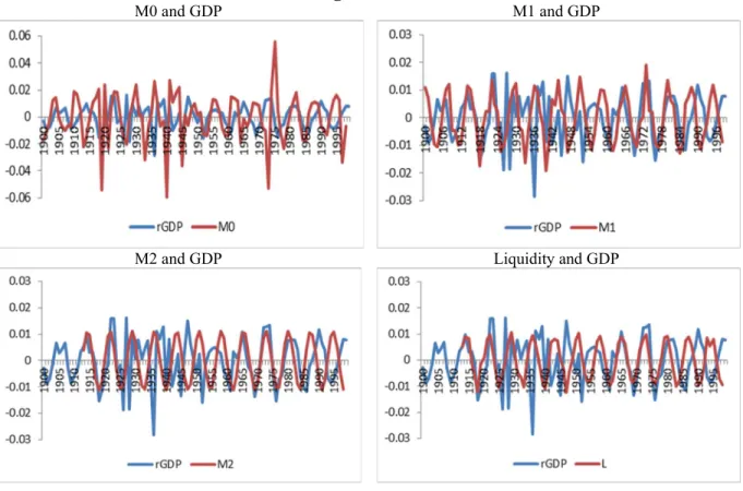
Then, following representations in Papademos and Stark (2010), we decompose GDP and monetary stocks into a low and high frequency component. To do so, we resort to Hamilton’s (2017) recent filtering approach. Economists and statisticians commonly use the Hodrick-Prescott filter. However, the criticisms surrounding the use of the HP filter (e.g. the possibility of generating spurious cycles) (Cogley and Nason, 1995) are well known. Figure 2.a presents the detrended levels of real GDP and real GDP per capita series for Portugal between 1900 and 1999. Figure 2.b replicates the same for our main monetary aggregates, namely the stocks of M0, M1, M2 and liquidity. Finally, Figure 2.c plots the high frequency components – or cycles - of M0, M1, M2 and liquidity against that of real GDP.
Starting around the end of the monarchy regime in 1910, the years that followed were marked by rapid economic growth up until around 1926 when Dr. Salazar took the power and the political regime changed from democratic to autocratic. A period of relatively smaller economic growth is visible during most of the 1930s but it started re-accelerating even the Second World War (a time when Portugal was heavily selling metals to Allied forces). Starting around 1950 until the late 1960s we entered a Golden Age (as in most other European nations). That period was characterized by significant structural changes in the Portuguese economy and capital deepening (Pereira and Lains, 2010). After that point the successive negative oil price shocks in the 1970s together with the 1974 Carnation Revolution - which ended the dictatorship regime – Portugal witnessed a phase of smaller growth (where human capital accumulation and productivity growth were the main driving factors). Never again, Portugal experienced such an extreme growth rate as during the Golden Age – with the exception being the relatively small hump visible in Figure
[7]
2.a around the mid-1980s associated with the adhesion of the country to the European Union in 1986.
Figure 2.a. Detrended Levels of real GDP and real GDP per capita, Portugal 1900-1999
To a great extent, the time dynamics of monetary aggregates followed the (inverse) behaviour of Portuguese’s GDP. as Figure 2.b illustrates, the rapid economic expansion after 1910 is reflected by a growth in money supply, which then decelerates in the 1930s and Second World War. Such money supply growth gains new momentum from the 1950s until the mid-1980s (despite such turbulent times in the 1970s), to then collapse in 1993 (when Portugal experienced an economic recession). That being said, in Figure 2.c we observe that the cycles of each monetary aggregate and that of real GDP were in many occasions synchronized.
Figure 2.b Low-frequency Component: Detrended series of M0, M1, M2 and Liquidity (L), Portugal 1900-1999
In Table 1 we report some descriptive statistics of real GDP’s average annual geometric growth rate using the sub-periods identified above. Confirming the visual inspection coming out of Figure 1.a and the historical justifications that followed, the period with the highest growth corresponds to 1926-1973 with an average of 4.3 percent per annum (reaching over 7 percent between 1961-1973). In contrast, the sub-period beginning with the Carnation Revolution up until mid-1980s was marked by negative average annual growth rates (-1.9 percent).
[8]
Figure 2.c High-Frequency Component: cyclical series of M0, M1, M2 against real GDP, Portugal 1900-1999
M0 and GDP M1 and GDP
M2 and GDP Liquidity and GDP
Table 1. Average Annual real GDP growth by time sub-periods, Portugal 1911-1999
Period Percent growth rate per annum Inter-period percent growth change 1911-1950 1.99 1950-1999 4.32 2.32 1911-1926 1.57 1926-1973 4.34 2.76 1974-1986 2.48 -1.86 1986-1993 3.82 1.34 1951-1985 4.55 1951-1960 4.24 1951-1973 5.81 1961-1973 7.01 1986-1999 3.73
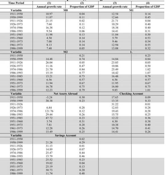
In Table 2, we repeat the previous exercise taking each of the main monetary aggregates so as to examine their behaviour around GDP’s reference time periods. The annual growth rate of M0, M1, M2 was the highest (above 20 percent) between 1911-1926. Also in this period, both checking and savings accounts grew above 30 percent annually. As for liquidity and net assets abroad the highest growth was experienced in the 1974-1986 period. Looking at column 2, the importance of monetary aggregates in proportion to GDP increased several fold between the 1911-1950 and the 1950-1999 periods (e.g. M0 went from a proportion to GDP of only 0.4 to 0.11; M2 went from a proportion to GDP of 0.23 to 0.84). finally, the weighted inter-period growth effect of M2 and liquidity was the highest (13.03 and 20.95, respectively) in the 1974-1986 period, when Portugal’s new democracy was taking the necessary steps to join the European Economic Community (EEC). All in all, it is clear that in several occasions money changes were associated with changes in real economic activity.
[9]
Table 2. Descriptive Statistics of different Monetary Aggregates (analysed over GDP reference time periods), Portugal 1911-1999
Time Period (1) (2) (3) (4)
Annual growth rate Proportion of GDP Annual growth rate Proportion of GDP
Variable M0 M1 1911-1950 10.97 0.04 12.54 0.14 1950-1999 11.07 0.11 12.66 0.45 1911-1926 21.15 0.02 21.71 0.04 1926-1973 7.60 0.11 10.29 0.40 1974-1986 16.38 0.12 18.38 0.40 1986-1993 9.54 0.06 14.41 0.31 1951-1985 11.98 0.13 11.84 0.50 1951-1960 4.50 0.14 5.79 0.53 1951-1973 7.00 0.14 9.46 0.54 1961-1973 8.13 0.14 12.94 0.55 1986-1999 7.48 0.05 13.08 0.32 Variable M2 L 1911-1950 0.21 0.23 1950-1999 14.48 0.74 14.84 0.84 1911-1926 26.04 0.05 23.85 0.05 1926-1973 11.16 0.47 10.06 0.50 1974-1986 21.70 0.84 25.49 1.02 1986-1993 15.19 0.77 14.42 1.07 1951-1985 15.21 0.73 16.48 0.79 1951-1960 6.56 0.57 6.56 0.57 1951-1973 11.94 0.67 11.95 0.67 1961-1973 16.78 0.75 16.80 0.75 1986-1999 12.23 0.79 9.85 1.01
Variable Net Assets Abroad Checking Account 1911-1950 -3.24 0.30 17.65 0.09 1950-1999 38.38 0.23 13.35 0.33 1911-1926 31.22 0.01 1926-1973 6.84 0.28 12.83 0.28 1974-1986 121.76 0.12 19.43 0.28 1986-1993 29.44 0.26 15.75 0.25 1951-1985 47.72 0.23 12.22 0.36 1951-1960 3.74 0.31 6.30 0.38 1951-1973 7.81 0.28 10.38 0.40 1961-1973 12.28 0.26 14.70 0.41 1986-1999 15.49 0.25 14.41 0.26
Variable Savings Account
1911-1950 0.02 1950-1999 21.28 0.29 1911-1926 31.13 0.01 1926-1973 14.89 0.07 1974-1986 25.47 0.44 1986-1993 15.79 0.46 1951-1985 25.52 0.23 1951-1960 19.02 0.04 1951-1973 25.19 0.13 1961-1973 30.73 0.20 1986-1999 11.74 0.48
Notes: Column (1) is calculated as the geometric annual growth rate over the specified period; Column (2) is the share in GDP averaged over the specified period.
To analyse these monetary time series in terms of their business cycle behaviour, we follow Correia et al. (1992) approach. Relying on the same set of reference sub-periods, we summarize in Table 3 the most important second moments of the different monetary aggregates. A few comments are worth making: i) most variables are more volatile than real GDP, in particular Net Assets Abroad (with the exceptions of liquidity and savings account whose relative standard deviations are below 1); ii) most series display a high degree of serial correlation; iii) most monetary aggregates are countercyclical (i.e., their contemporaneous correlation with real GDP is negative) with the exceptions of checking account); iv) most monetary aggregates lead the economic cycle (i.e., the maximum correlation value between these variables at time t and GDPtj occurs for j>0), while checking account is a lagging variable.
[10]
Table 3. Second Moments of detrended Monetary Aggregates, Portugal 1911-1999
Time periods St.dev. real GDP St.dev. Variable Relative St. dev.
Autocorrelation Cross-Correlation real GDP (t) and Variable (t±j) 1 0 1 2 -1 -2 M0 1911-1999 0.0034 0.0124 3.56 0.57 -0.09 -0.19 0.20 0.09 -0.13 1910-1973 0.0039 0.0124 3.10 0.57 -0.02 -0.18 0.17 0.15 -0.19 1973-1999 0.0019 0.0125 6.44 0.56 -0.52 -0.49 0.49 0.14 -0.21 1910-1950 0.0047 0.0125 2.62 0.58 0.00 -0.08 0.09 0.08 -0.09 1950-1999 0.0018 0.0124 6.79 0.56 -0.33 -0.49 0.49 0.14 -0.21 M1 1911-1999 0.0034 0.0063 1.80 0.54 -0.10 -0.24 0.24 0.13 -0.15 1910-1973 0.0039 0.0063 1.57 0.54 -0.06 -0.19 0.17 0.10 -0.14 1973-1999 0.0019 0.0063 3.24 0.54 -0.29 -0.52 0.57 0.48 -0.49 1910-1950 0.0047 0.0063 1.32 0.55 -0.15 -0.15 0.13 -0.01 0.00 1950-1999 0.0018 0.0063 3.42 0.53 -0.05 -0.52 0.57 0.48 -0.49 M2 1911-1999 0.0034 0.0058 1.68 0.44 -0.60 -0.45 0.56 -0.06 0.21 1910-1973 0.0039 0.0059 1.47 0.44 -0.67 -0.45 0.55 -0.13 0.28 1973-1999 0.0019 0.0058 3.01 0.44 -0.43 -0.52 0.56 0.16 -0.05 1910-1950 0.0047 0.0059 1.24 0.45 -0.77 -0.49 0.64 -0.16 0.37 1950-1999 0.0018 0.0059 3.20 0.44 -0.42 -0.52 0.56 0.16 -0.05 L 1911-1999 0.0034 0.0028 0.80 0.44 -0.62 -0.37 0.49 -0.16 0.30 1910-1973 0.0039 0.0028 0.70 0.44 -0.69 -0.35 0.47 -0.25 0.39 1973-1999 0.0019 0.0028 1.44 0.43 -0.46 -0.50 0.55 0.12 -0.01 1910-1950 0.0047 0.0029 0.60 0.45 -0.80 -0.37 0.55 -0.31 0.50 1950-1999 0.0018 0.0028 1.54 0.44 -0.43 -0.50 0.55 0.12 -0.01
Net Assets Abroad
1911-1999 0.0034 0.0949 27.21 0.52 -0.24 -0.53 0.63 0.37 -0.26 1910-1973 0.0039 0.0413 10.34 0.51 0.44 -0.22 0.12 0.54 -0.59 1973-1999 0.0019 0.1304 67.15 0.52 -0.43 -0.55 0.68 0.40 -0.27 1910-1950 0.0047 0.0158 3.30 -0.52 -0.94 0.64 0.37 -0.53 1.00 1950-1999 0.0018 0.0978 53.40 0.52 -0.24 -0.55 0.68 0.40 -0.27 Current Accounts 1911-1999 0.0034 0.0087 2.51 0.28 0.12 -0.30 0.08 0.37 -0.31 1910-1973 0.0039 0.0088 2.20 0.27 0.06 -0.44 0.22 0.47 -0.33 1973-1999 0.0019 0.0090 4.62 0.30 0.56 0.07 -0.37 0.22 -0.44 1910-1950 0.0047 0.0087 1.82 0.27 -0.02 -0.51 0.32 0.50 -0.29 1950-1999 0.0018 0.0088 4.79 0.29 0.49 0.07 -0.37 0.22 -0.44 Savings Accounts 1911-1999 0.0034 0.0033 0.94 0.60 -0.06 -0.01 -0.03 -0.06 0.05 1910-1973 0.0039 0.0033 0.81 0.59 -0.12 -0.10 0.08 -0.02 0.00 1973-1999 0.0019 0.0033 1.72 0.62 0.14 0.12 -0.23 -0.38 0.36 1910-1950 0.0047 0.0033 0.69 0.59 0.01 -0.08 0.05 0.08 -0.10 1950-1999 0.0018 0.0033 1.80 0.60 -0.22 0.12 -0.23 -0.38 0.36
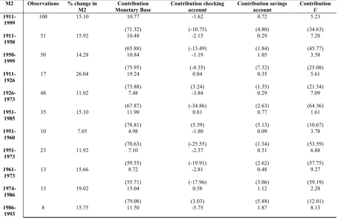
Our final exercise in this section tries to uncover the proximate determinants of the two most relevant monetary aggregates, M1 and M2. The monetary stock is defined as the set of assets owned by economic agents which, at a given moment in time, satisfy three main roles: store of value, unit of account, and medium of exchange. The monetary emissions by the Portugal’s Central Bank – denoted monetary base – is composed of coins and bills owned by economic agents – currency in circulation – and of the central bank’s financial responsibilities next to commercial banking institutions – that is, reserves. The monetary emissions by commercial banks contains economic agents’ deposits. In other words, the monetary stock can be defined as the product between the monetary base and the money multiplier. The monetary base is determined by actions from the monetary authority and the multiplier summarizes the banks’ behaviour, as far as the liquidity of their assets is concerned and the general public’s behaviour, as far as the distribution of monetary balances through different assets is concerned. In this context, following Santos (1994), we compute the absolute and relative contributions of the proximate determinants to changes in the monetary stock. Looking at Tables 4 a and 4b, between 1911-1999, M1 grew at the annual rate of 12.6 percent and M2 at 15.1 percent. The monetary base grew at the average annual rate of 10.8 percent, contributing around 86 percent to the overall growth of M1 and around 71 percent to the overall growth of M2. Savings accounts contributed 4.8 percent to M2’s growth. All in all, the largest share is attributed to the monetary base. However, an analysis of
[11]
relevant sub-periods reveals that, in some cases, other proximate determinants had a stronger and more significant influence in the growth of either M1 or M2.
Table 4a. Absolute and relative contribution of the proximate determinants to changes in monetary stock M1, Portugal 1911-1999
M1 Observations % change in M1 Contribution Monetary Base Contribution checking account Contribution U
1911-1999 100 12.60 10.77 -1.62 3.45 (85.50) (-12.89) (27.39) 1911-1950 51 12.54 10.48 -2.15 4.21 (83.58) (-17.11) (33.53) 1950-1999 50 12.49 10.84 -1.19 2.84 (86.79) (-9.54) (22.75) 1911-1926 17 21.11 19.24 0.84 1.03 (91.11) (3.99) (4.89) 1926-1973 48 10.13 7.48 -3.84 6.49 (73.85) (-37.93) (64.08) 1951-1985 35 11.84 11.90 0.81 -0.87 (100.49) (6.87) (-7.36) 1951-1960 10 6.39 4.98 -1.80 3.21 (77.90) (-28.18) (50.28) 1951-1973 23 9.57 7.10 -2.37 4.84 (74.16) (-24.80) (50.64) 1961-1973 13 12.01 8.72 -2.81 6.10 (72.63) (-23.42) (50.79) 1974-1986 13 15.43 15.04 0.58 -0.18 (97.46) (3.74) (-1.20) 1986-1993 8 17.12 11.50 -5.75 11.37 (67.16) (-33.59) (66.43) 1986-1999 14 14.85 8.84 -6.18 12.19 (59.55) (-41.61) (82.06)
Note: For each time period, the first row indicates the absolute contribution and the second row (in parenthesis) the relative contribution. The term u is a residual which translates the change in M, explained by the interaction between the changes of the different determinants considered. % change rates are annual averages. Take LnMt the natural logarithm of the monetary stock at time t and take LnMs|x the natural logarithm of the stock at time s, given that only the determinant x has changed between t and s. The difference LnMs|x- LnMt translates the rate of change in M that is imputable to the change in x, that is, its absolute contribution to the change in M between s and t. The relative contribution is given by the ratio between the absolute contribution and the change that has indeed occurred in M, LnMs- LnMt.
Table 4b. Absolute and relative contribution of the proximate determinants to changes in monetary stock M2, Portugal 1911-1999
M2 Observations % change in
M2 Monetary Base Contribution Contribution checking account Contribution savings account Contribution U 1911-1999 100 15.10 10.77 -1.62 0.72 5.23 (71.32) (-10.75) (4.80) (34.63) 1911-1950 51 15.92 10.48 -2.15 0.29 7.28 (65.88) (-13.49) (1.84) (45.77) 1950-1999 50 14.28 10.84 -1.19 1.05 3.58 (75.95) (-8.35) (7.32) (25.08) 1911-1926 17 26.04 19.24 0.84 0.35 5.61 (73.88) (3.24) (1.35) (21.54) 1926-1973 48 11.02 7.48 -3.84 0.29 7.09 (67.87) (-34.86) (2.63) (64.36) 1951-1985 35 15.10 11.90 0.81 0.77 1.61 (78.81) (5.39) (5.13) (10.67) 1951-1960 10 7.05 4.98 -1.80 0.09 3.78 (70.63) (-25.55) (1.34) (53.59) 1951-1973 23 11.92 7.10 -2.37 0.31 6.88 (59.55) (-19.91) (2.62) (57.75) 1961-1973 13 15.66 8.72 -2.81 0.48 9.27 (55.71) (-17.96) (3.06) (59.19) 1974-1986 13 19.02 15.04 0.58 1.12 2.28 (79.08) (3.03) (5.88) (12.01) 1986-1993 8 15.75 11.50 -5.75 1.87 8.13
[12]
(73.00) (-36.51) (11.87) (51.64)
1986-1999 14 12.81 8.84 -6.18 1.85 8.29
(69.06) (-48.25) (14.45) (64.74)
Note: see note of Table 4a.
5. Econometric Results
Table 5 presents our results for the unit root and structural break testing and it is organized by grouping each type of variables together under a specific heading. Both the ADF and PP variants are performed for series in levels (columns 1 and 3) and first-differences (columns 2 and 4). In column (5) we show the results of the ZA test and in columns (6), (7) and (8) the VP, Perron and Yabu (2009) (PY) and CMR tests, respectively. Results support the presence of a single unit root in all time series, i.e., each series is first-differenced stationary. Moreover, paying special attention to the identified breaks, many of these dates have clear correspondence to relevant moments of the Portuguese economic history. For example, looking at the GDP series, several tests uncover the years of 1974/1975 associated with the period around the Carnation Revolution or the year of 1927 around the time Dr. Salazar was elected Prime Minister or the year of 1940 corresponding to the early period of the Second World War.
Table 5. Unit Root Tests and Structural Breaks, Portugal 1911-1999
Series Period Time
ADF PP
ZA VP(AO) PY2009 CMR(AO) Levels differences First Levels First differences
(0) (1) (2) (3) (4) (5) (6) (7) (8)
Gross Domestic Product Series Real GDP 1911-1999 -2.83 -11.29*** -2.87 -11.26*** 1935 1975 1949 1948, 1974 Real GDP pc 1911-1999 -2.16 -10.90*** -2.23 -10.98*** 1935 1975 1951 1952, 1981 Nominal GDP 1911-1999 -2.86 -0.83 -1.58 -6.80*** 1948 1993 1969 1961, 1981 Monetary Aggregate Series M0 1911-1999 -3.31* -4.09*** -2.60 -6.81*** 1931 1976 1972 1925, 1976 M1 1911-1999 -2.72 -4.39*** -2.26 -4.40*** 1952 1990 1970 1925, 1974 M2 1911-1999 -2.59 -3.71** -1.91 -3.76** 1947 1973 1965 1945, 1978 L 1911-1999 -2.29 -3.75** -1.66 -3.72** 1943 1979 1960 1947, 1981 Net assets abroad 1947-1999 2.77 -9.89*** -3.49* -8.79*** 1980 1981 1978** 1981, 1989 Total USD reserves 1947-1999 -2.71 -6.40*** -2.71 -6.41*** 1980 1981 1978 1965, 1981 Price Series Price deflator 1911-1993 -3.05 -2.856 -1.69 -4.90*** 1959 1980 1972 1925, 1981
Note: All variables are in logs. The null in ADF and PP tests is of unit root. ADF critical values: 4028, 3.445, -3.145 for 1, 5 and 10% levels respectively. The null in the remaining break-type tests is of unit root against the break stationary alternative hypothesis. The ZA test statistic reported is the minimum Dickey-Fuller statistic calculated across all possible breaks in the series, when both a break in the intercept and the time trend is allowed for. The year in parenthesis denotes the year when this minimum DF statistic is obtained. The 1% critical value is -5.57 and the 5% critical value is -5.08. As for the VP test, “AO” means addictive outlier and critical values are taken from Perron and Vogelsang (1992), in particular, -3.56 (AO) for 5% level. In column 7 we ran the Perron and Yabu (2009) (PY) unit root test. As for CMR the 5% critical value is -5.49, also taken from Perron and Vogelsang (1992).
Now that the order of integration has been assessed, we are in a position to check whether real GDP and our different monetary aggregates are cointegrated. The Johansen-Juselius’ trace and max-Eigen value statistics are displayed in Table 6 and support the existence of linear combinations of these variables which are stationary. The existence of a long-run cointegrating relationship between GDP and monetary aggregates provides evidence of money non-neutrality in Portugal over this very long time span. As has been emphasize by Bruggemann et al. (2003), it is important to formally investigate the stability of the cointegrating vectors once a long-run relationship has been identified. Hansen and Johansen (1993) outlined a procedure that formally tests the constancy of cointegrating vectors in the context of Full Information Maximum Likelihood estimations. Results from the Hansen-stability test (available upon request) do not reject the null hypothesis that the series are cointegrated (p-values larger than 20 percent). We
[13]
further tested the hypothesis of a structural shift in the cointegration relationships found above, by using the Gregory and Hansen (1996) regime shift procedure. Table A1 presents our results. After taking into account the possibility of breaks in the cointegrating series, we get for the GDP-monetary aggregate relationship, rejections of the null of no cointegration for the ADF* and *
Z
statistics (in line with previous findings). We also checked the variance decompositions over a forecast horizon of three and six years. Results available upon request confirm the influence of the money supply over output. For the period 1911-1999, money supply shocks explain, over a period of six years, between 10-18 percent of the variance of real GDP’s forecast error (depending on whether one focuses on M0, M1 or M2). Moreover, innovations in M0, M1 and M2 explain, for the same period, an important fraction of the variance of GDP deflator’s forecast error (between 9-26 percent). These results reinforce the findings obtained via the causality tests above. Shocks to changes in real GDP and GDP deflator, on the other hand, explain only a small fraction of the variance observed in changes in monetary aggregates. That fraction however increased in the post-1974 period.
Table 6. Johansen-Juselius Cointegration Tests, Portugal 1911-1999
Null Alternative 5% Critical
Value Variable Pairs
GDP+M0 GDP+M1 GDP+M2 GDP+L GDP+Net Assets Abroad trace 0 r r 1 20.26 23.54* 28.237* 38.27* 36.02* 19.80 1 r r 2 9.16 7.93 5.90 5.93 8.49 2.56 max 0 r r1 15.89 15.61* 22.33* 32.33* 27.53* 17.24* 1 r r2 9.16 7.93* 5.90 5.93 8.49 2.56 Cointegration* Yes Yes Yes Yes Yes
Note: * denotes rejection of the null hypothesis at the 0.05 level Critical Value based on MacKinnon-Haug-Michelis p-values.
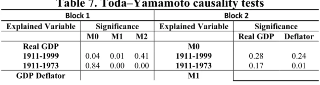
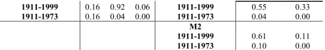
To assess causality we estimate a five variable VAR(2) - which included real GDP, GDP deflator, M0, M1, M2 from 1911-1999. 12 This Choleski ordering was followed. Looking at Table
7, we get at the 1 percent significance level that for the period 1911-1973, M1 and M2 Granger-caused real GDP. Focusing on the period 1974-99, our results show that changes in M1 and M2 Granger-caused changes in the GDP deflator. For other time periods and considering both M0 and M2, money growth seems to have remained non-inflationary. The second block suggests that changes in output did not Granger-cause changes in the money supply (with the exception of the most recent period 1974-99 for M2). All in all, evidence seems to support that, contrarily to Keynesian economists’ claim, causality does not run from real GDP to money and between 1911-1999 money supply was not neutral. As for the influence of prices on the money supply, with the exception of the cases of M0 and M1, prices seemed to have Granger-caused changes in M2, that is, movements in the money supply were not independent from past movements in the price level.
Table 7. Toda–Yamamoto causality tests
Block 1 Block 2
Explained Variable Significance Explained Variable Significance M0 M1 M2 Real GDP Deflator Real GDP M0 1911-1999 0.04 0.01 0.41 1911-1999 0.28 0.24 1911-1973 0.84 0.00 0.00 1911-1973 0.17 0.01 GDP Deflator M1 _____________________________
12 The lag length criteria suggested 2 lags as the appropriate lag-structure. Note that even though a cointegrating relationship was found, one cannot Granger-test in a VECM environment. For this reason, we use first a VAR to uncover causality implications and then estimate a proper VECM to look at impulse response functions.
[14] 1911-1999 0.16 0.92 0.06 1911-1999 0.55 0.33 1911-1973 0.16 0.04 0.00 1911-1973 0.04 0.00 M2 1911-1999 0.61 0.11 1911-1973 0.10 0.00
Note: In these tests, we used the rate of change of each variable under scrutiny. The null is of no causality. The period 1974-1999 is too short to carry out the Toda-Yamamoto tests (refer to the main text for further details).
Since we uncovered existing of cointegrating relationships in Table 6, the next step is to estimate a VECM(2) with the same Choleski structure of variables and inspect the responses of the different endogenous variables to various shocks.
Figure 3. VECM Impulse Response Functions
-.005 .000 .005 .010 .015 .020 .025 1 2 3 4 5 6 7 8 9 10 RGDP DEFLATOR M0 M1 M2 Response of RGDP to Cholesky One S.D. Innovations -.02 .00 .02 .04 .06 .08 1 2 3 4 5 6 7 8 9 10 RGDP DEFLATOR M0 M1 M2
Response of DEFLATOR to Cholesky One S.D. Innovations -.02 .00 .02 .04 .06 .08 1 2 3 4 5 6 7 8 9 10 RGDP DEFLATOR M0 M1 M2 Response of M0 to Cholesky One S.D. Innovations -.02 .00 .02 .04 .06 .08 1 2 3 4 5 6 7 8 9 10 RGDP DEFLATOR M0 M1 M2 Response of M1 to Cholesky One S.D. Innovations -.02 .00 .02 .04 .06 .08 .10 1 2 3 4 5 6 7 8 9 10 RGDP DEFLATOR M0 M1 M2 Response of M2 to Cholesky One S.D. Innovations
[15]
Figure 3 shows the impulse responses to one standard deviation shocks. Each chart plots the response of the title variable to various shocks identified in the legend. A positive shock of real GDP will lead to an increase in the inflation, as one normally would expect. Also, the positive variation of real GDP will trigger a positive variation the various monetary aggregates. Following a positive shock on inflation, the response of the M2 monetary aggregate is the one of growing the money supply, unlike the theoretical hypotheses according to which an unexpected price increase leads to a fall in money supply. However, this contradiction was also observed by Kim and Roubini (2000). The inflation persistence will disappear after 7 months. A positive variation of the monetary aggregate M2 will trigger both a short run increase in real GDP and the price level, however, as the horizon increases, these responses die out and even become negative.
Finally, in Figure 4 we plot the impulses responses stemming from a BVAR model – with a Koko-Minnesota/Litterman prior. A positive inflation shock leads to a slightly negative response of real GDP and, by the same token, a positive shock of real GDP leads to a short run negative effect on prices, to recover (and become positive) after 3-4 years. Moreover, a positive shock of real GDP leads to positive changes in all monetary aggregates in a persistent way. All in all, evidence seems to support the clear interdependence between output and money in Portugal.
6. Conclusion
The transmission mechanism through which changes in the money supply affect output is of great importance because it helps determining the costs (in terms of unemployment) of appropriately using monetary policy for stabilization purposes. This paper, revisits the empirical debate between monetarists and Keynesians by testing money’s (non-)neutrality. Focusing on the Portuguese case over a long time span between 1911-1999 (the life span of the currency Escudo), we carry out a thorough examination of the dynamics of several monetary aggregates over Portuguese’s historical real business cycles. We also employ several time series econometric techniques to formally test whether output and money supply are cointegrated, to assess the direction of causality between these variables and evaluate the responses to various shocks by estimating VECMs and Bayesian VARs. We also devoted special attention to robustness checks, which included considering structural breaks and regime changes in our time series of interest.
This work has had as objective to provide new empirical results in the transmission mechanisms of monetary policy in Portugal, using modern techniques. We found that on several occasions (depending on the exact monetary aggregate and time period considered), money changes were associated with changes in real economic activity. Most monetary aggregates are more volatile than GDP, display high serial autocorrelation, are generally countercyclical and lead the economic cycle (except checking accounts). Moreover, growth in the monetary base is the money determinant most contributes to absolute and relative changes in the monetary stock. Finally, we uncovered that our monetary series were characterized by unit roots and were cointegrated with real GDP (after accounting for endogenously estimated breaks). Evidence suggested that money supply Granger-caused real GDP supporting the money non-neutrality hypothesis in the case of Portugal. Forecast error variance decompositions confirmed the influence of money over output. Finally, impulse response function analyses uncovered a persistent and mutual effect running from a shock in real GDP to monetary aggregates and vice versa.
[16]
Figure 4. Bayesian VAR Impulse Response Functions, Koko Minnesota/Litterman Prior -.005 .000 .005 .010 .015 .020 .025 1 2 3 4 5 6 7 8 9 10 RGDP DEFLATOR M0 M1 M2 Response of RGDP to Cholesky One S.D. Innovations -.01 .00 .01 .02 .03 .04 1 2 3 4 5 6 7 8 9 10 RGDP DEFLATOR M0 M1 M2
Response of DEFLATOR to Cholesky One S.D. Innovations .00 .01 .02 .03 .04 .05 .06 1 2 3 4 5 6 7 8 9 10 RGDP DEFLATOR M0 M1 M2 Response of M0 to Cholesky One S.D. Innovations .00 .01 .02 .03 .04 1 2 3 4 5 6 7 8 9 10 RGDP DEFLATOR M0 M1 M2 Response of M1 to Cholesky One S.D. Innovations .000 .005 .010 .015 .020 .025 .030 1 2 3 4 5 6 7 8 9 10 RGDP DEFLATOR M0 M1 M2 Response of M2 to Cholesky One S.D. Innovations
[17] References
1. Abbas, K. (1991), “Causality Test Between Money and Income: A Case Study of Selected Developing Asian Countries (1960- 1988)”, Pakistan Development Review, (30).
2. Abdulrazag, B., Shotar, M., Al-Quran, A. (2003), “Money Supply in Qatar: An Empirical Investigation”, Journal of Economic and Administrative Sciences, 18(2).
3. Abel, A., Bernanke, B. (2005), “Macroeconomics”, 5th edn, Reading, MA, Pearson Addison Wesley.
4. Amaral, L. (2009), "New Series for GDP Per Capita, Per Worker, and Per Worker-Hour in Portugal, 1950-2007," Working Paper Faculty Economics, New University of Lisbon, 2009.
5. Baptista, D., C. Martins, M. Pinheiro, and P. Reis (1997), “New Estimates for Portugal's GDP, 1910-1958”, História Económica, Banco de Portugal, 7.
6. Bednarik, R. (2010), “Money Supply and real GDP: The case of the Czech Republic”.
7. Belongia, M. T. (1996), “Measurement Matters: Recent Results from Monetary Economics Reexamined.” Journal of Political Economy 104, 1065-1083
8. Berger H, Österholm P (2008), “Does Money Matter for U.S. Inflation? Evidence from Bayesian VARs”. International Monetary Fund Working Paper/08/76.
9. Borio, C. and Disyatat, P. (2010), “Unconventional Monetary Policies: An Appraisal”, The Manchester School, 78(1), 53-89.
10. Brandt P.T., Freedman J.R. (2006), “Advances in Bayesian Time Series Modelling and the Study of Politics: Theory Testing, Forecasting, and Policy Analysis”. Political Analysis, 14, 1-36.
11. Bruggeman, A., P. Donati, and A. Warne (2003), “Is the Demand for Euro Area M3 Stable?”, European Central Bank - Working Paper Series, No. 255.
12. Brunner K., and A. H. Meitzer (1976),” An aggregative theory for a closed economy, and, Monetarism: The principal issues, areas of agreement and the work remaining”, in: Jerome Stein, ed., Monetarism (Amsterdam).
13. Carpenter, S. and Demiralp, S. (2012), “Money, reserves, and the transmission of monetary policy: Does the money multiplier exist?”, Journal of Macroeconomics, 34, 59–75.
14. Clemente, J., Montanes, A., Reyes, M. (1998), “Testing for a unit root in variables with a double change in the mean”, Economics Letters 59, 175-182.
15. Cogley, T., and Nason, J. M. (1995), “Effects of the Hodrick-Prescott filter on trend and difference stationary time series: Implications for business cycle research”, Journal of Economic Dynamics and Control, 19, 253--278.
16. Correia, I., Neves, J. C., Rebelo, S. (1992), "Business Cycles from 1850-1950: new facts about old data", European Economic Review, 36, 459-467.
17. Daniela Z., and Mihail I. (2010), “Linking Money Supply with Gross Domestic Product In Romania”, Annales Universitatis Apulensis Series Oeconomica, 12(1)
18. Darrat, A. F., M. C. Chopin and B. J. Bento (2005), “Money and Macroeconomic Performance: Revisiting Divisia Money”, Review of Financial Economics, 93-101.
19. Fisher, I. (1911), “The Purchasing Power of Money: Its Determination and Relation to Credit, Interest, and Crises”, Macmillan, New York.
20. Friedman, B. and Kuttner, K. (1992), “Money, income, prices and interest rates”, American Economic Review, 82, 472-492.
21. Friedman, M. (1974), “Comments on the Critics”, In: Gordon, Robert J., Editor, 1974. Milton Friedman's Monetary Framework, University of Chicago Press, Chicago.
22. Friedman, M. A. and Schwartz, A. J. (1963), “A Monetary History of the United States, 1867– 1960”, Princeton University Press, Princeton, NJ.
23. Gedeon, S. (1985), “The Post Keynesian Theory of Money: a summary and an Eastern European Example”, Journal of Post Keynesian Economics, 8(2), 208-221.
24. Giannone, D., Lenza, M., Reichlin, R. (2012), “Money, credit, monetary policy and the business cycle in the Euro area”, ECARES Working Paper 2012–008.
25. Granger, C. W. J. (1969), “Investigating causal relations by econometric models and cross spectral methods”, Econometrica, 37, 424- 38
26. Gregory, A. W. and B. E. Hansen (1996), “Residuals-based tests for cointegration in models with regime shifts”. Journal of Econometrics, 70, 99-126
[18]
27. Hamilton, J. (2017), “Why You Should Never Use the Hodrick-Prescott Filter," NBER WP 23429.
28. Hansen, H. and Johansen, S. (1993), “Recursive estimation in cointegrated models”, Institute of Mathematical Statistics, Reprint No. 1, University of Copenhagen, Denmark.
29. Hodgeman, D. (1960), “Soviet monetary controls through the banking system”, in Gregory Grossman, Ed. Value and Plan, pp. 105-124. Berkeley, University of California Press.
30. Howells, P. (1995), “The demand for endogenous money”, Journal of Post Keynesian Economics, 18(1), 89-106
31. Hume, D. (1875), “Essays, Moral, Political, and Literary”, Ed. T. H. Green and T. H. Gorse. Longmans Green, London.
32. Hussain, F. and Abbas, K. (2000), “Money, Income, Prices, and Causality in Pakistan: A Trivariate Analysis”, Pakistan Development Review,178.
33. Johansen, S. and Juselius, K. (1990), “Maximum Likelihood Estimation and Inference on Cointegration – with Applications to the Demand for Money”, Oxford Bulletin of Economics and Statistics 52, 169-210.
34. Joshi, K., and Joshi S. (1985), “Money, Income, and Causality: A Case Study for India”. Arthavikas.
35. Kalulumia, P. and Yourogou, P. (1997), “Money and Income Causality in Developing Economies: a Case Study of Selected Countries in Sub-Saharan Africa”, Journal of African Economics, 6.
36. Khan, A., and Siddiqui A. (1990). “Money, Prices and Economic Activity in Pakistan: A Test of Causal Relation. Pakistan Economic and Social Review, 121-136
37. Lee, S., and Li W. (1983), “Money, Income, and Prices and their Lead-lag Relationship in Singapore”. Singapore Economic Review, 73–87.
38. Litterman R.B. (1980), “A Bayesian Procedure for Forecasting with Vector Autoregressions”. Unpublished mimeo.
39. Locke, J. (1691), “Some considerations on the consequences of the lowering of interest and the raising of the value of money”, Marxists
40. Maddison, A. (1987), “Growth and Slowdown in Advanced Capitalist Countries: Techniques of Quantitative Assessment”, Journal of Economic Literature 25(2), 649–98.
41. Maddison, A. (2001), “The World Economy: A Millennial Perspective”. Paris: OECD.
42. Mallick KS, Sousa R (2009), “Monetary Policy and Economic Activity in the BRICS”. NIPE Working Paper Series 27.
43. Mata, E., and N. Valério (1993), “História Económica de Portugal - Uma Perspectiva Global”, Editorial Presença, Lisboa.
44. McLeay, M., Radia, A. and Thomas, R. (2014), “Money creation in the modern economy”, Bank of England Quarterly Bulletin, 54(1), 14–27.
45. Migliardo C (2010), “Monetary Policy Transmission in Italy: A BVAR Analysis with Sign Restriction”, Czech Economic Review, 4(2), 139- 167.
46. Mill, J. S. (1848), “Principles of Political Economy”, J. W. Parker, London
47. Mishkin, F. (2004), “The economics of money, banking and financial markets”, 7th edn, Reading,
MA, Addison Wesley.
48. Moore, B. J. (1988), “Horizontalists and Verticalists: The Macroeconomics of Loans Money” (New York: Cambridge University Press).
49. Obaid, G. (2007), “Money Supply-Output Causality in Egypt”, Faculty of Commercial and Business Administration Magazine, Helwan University.
50. Ogunmuyiwa M., and Ekone, F. (2010), “Money Supply- Economic Growth Nexus in Nigeria”, Olabisi Onabanjo University, 22(3).
51. Palley, T. (1996), “Post Keynesian Economics: debt, distribution and the macroeconomy”, MacMillan.
52. Papademos L.D., Stark J. (2010) Enhancing Monetary Analysis, European Central Bank.
53. Pereira, A., and Lains, P. (2010), “From an agrarian society to a knowledge economy: Portugal 1950-2010”, Universidad Carlos III de Madrid Working Papers, No. 10-09.
54. Perron, P. (1989), “The Great Crash, the Oil Price Shock, and the Unit Root Hypothesis,” Econometrica 57, 1361-1401.
55. Perron, P. and Vogelsang, T. J. (1992), “Nonstationarity and level shifts with an application to purchasing power parity”, Journal of Business and Economic Statistics, 10, 301-320.
[19]
56. Perron, P. and Yabu, T. (2009), “Testing for Shifts in Trend with an Integrated or Stationary Noise Component”, Journal of Business and Economics Statistics, 27, 369-396.
57. Pickersgill, J. (1976), “Financial Planning in the Soviet Economy”, in Judith Thornton, Ed. Economic Analysis of the Soviet-type System, pp. 141-155. Cambridge University Press.
58. Portes, R. (1983), “Central Planning and Monetarism: fellow travellers?”, in Padman Desai, Ed. Marxism, Central Planning and the Soviet Economy, pp. 149-165. Cambridge MIT Press.
59. Portes, R., and Santorum, A. (1987), “Money and the Consumption Goods Market in China.” Journal of Comparative Economics, 11(3), 354-371,
60. Reis, J. (1990), “A Evolução da Oferta Monetária Portuguesa 1854-1912”, Série História Económica, Banco de Portugal.
61. Santos, F. T. (1994), “Stock monetario e desempenho macroeconomico durante o Estado Novo”, Analise Social, 12, 981-1003.
62. Sims CA, Zha T (1998), “Bayesian Methods for Dynamic Multivariate Models”, International Economic Review, 39(4), 949-968.
63. Sims, C. A. (1972), “Money, income and causality”, American Economic Review, 62, 540-52. 64. Tan, H. B. and Baharumshah, A. Z. (1999). “Dynamic Causal Chain of Money, Output, Interest Rate and Prices in Malaysia: Evidence Based on Vector Error-Correction Modelling Analysis”. International Economic Journal, 13 (1), 103-120.
65. Toda, H.Y. and Phillips, P.C.B. (1994), “Vector Autoregressions and Causality: A Theoretical Overview and Simulation Study,” Econometric Reviews 13, 259-285
66. Toda, H.Y. and Yamamoto, T. (1995), “Statistical inference in Vector Autoregressions with possibly integrated processes”, Journal of Econometrics, 66, 225-250.
67. Vogelsang, T. (2001), “Testing for a Shift in Trend When Serial Correlation is of Unknown Form,” Unpublished Manuscript, Department of Economics, Cornell University.
68. Vogelsang, T. J. and Perron, P. (1998), “Additional tests for a unit root allowing for a break in the trend function at an unknown time”, International Economic Review, 39, 1073-1100.
69. Walsh, C. (2003), “Monetary Theory and Monetary Policy”, 2nd edn, Cambridge, MA, MIT Press.
70. Wary, L.R. (1990), “Money and Loans in Capitalist Economies: The Endogenous Money Approach” (Northampton MA: Edward Elgar Publishing).
71. Zivot, E. and Andrews, K. (1992), “Further Evidence on The Great Crash, The Oil Price Shock, and The Unit Root Hypothesis”, Journal of Business and Economic Statistics, 10 (10), 251–70.
[20] APPENDIX
Table A1. Testing for regime shifts in cointegration: Gregory-Hansen
Relation Real GDP and Monetary Aggregates Type of test ADF test Phillips Test
*
ADF stat Estimated break date *
Z stat Estimated break date GDP+M0 -5.02** 1976 -89.43** 1972 GDP+M1 -4.86** 1970 -109.11** 1974 GDP+M2 -6.04** 1973 -96.63** 1978 GDP+L -6.29** 1979 -88.95** 1981 GDP+Net Assets Abroad -5.3*** 1980 -107.05** 1981
Note: ADF*and *
Z refer to the Augmented Dickey-Fuller (ADF) and to the Phillips *
Z tests statistics; null of no
cointegration. ** denotes significance at the 5 percent level or lower, using the critical values from Gregory and Hansen (1996), table 1.
[21]
Figure A1. Bayesian VAR Impulse Response Functions, Sims and Zha Prior
-.005 .000 .005 .010 .015 .020 .025 1 2 3 4 5 6 7 8 9 10 RGDP DEFLATOR M0 M1 M2 Response of RGDP to Cholesky One S.D. Innovations -.01 .00 .01 .02 .03 .04 1 2 3 4 5 6 7 8 9 10 RGDP DEFLATOR M0 M1 M2
Response of DEFLATOR to Cholesky One S.D. Innovations .00 .01 .02 .03 .04 .05 .06 1 2 3 4 5 6 7 8 9 10 RGDP DEFLATOR M0 M1 M2 Response of M0 to Cholesky One S.D. Innovations .00 .01 .02 .03 .04 1 2 3 4 5 6 7 8 9 10 RGDP DEFLATOR M0 M1 M2 Response of M1 to Cholesky One S.D. Innovations .005 .010 .015 .020 .025 .030 1 2 3 4 5 6 7 8 9 10 RGDP DEFLATOR M0 M1 M2 Response of M2 to Cholesky One S.D. Innovations