Thermo-hydro-mechanical processes in fractured rock formations during a glacial advance

www.geosci-model-dev.net/8/2167/2015/ doi:10.5194/gmd-8-2167-2015

© Author(s) 2015. CC Attribution 3.0 License.

Thermo-hydro-mechanical processes in fractured rock formations

during a glacial advance

A. P. S. Selvadurai1, A. P. Suvorov1, and P. A. Selvadurai2

1_{Department of Civil Engineering and Applied Mechanics, McGill University, Montréal, QC, H3A 0C3, Canada} 2_{Department of Civil and Environmental Engineering, University of California, Berkeley, CA 94720, USA} Correspondence to:A. P. S. Selvadurai ([email protected])

Received: 12 October 2014 – Published in Geosci. Model Dev. Discuss.: 5 November 2014 Revised: 25 June 2015 – Accepted: 26 June 2015 – Published: 20 July 2015

Abstract. The paper examines the coupled thermo-hydro-mechanical (THM) processes that develop in a fractured rock region within a fluid-saturated rock mass due to loads im-posed by an advancing glacier. This scenario needs to be ex-amined in order to assess the suitability of potential sites for the location of deep geologic repositories for the storage of high-level nuclear waste. The THM processes are examined using a computational multiphysics approach that takes into account thermo-poroelasticity of the intact geological forma-tion and the presence of a system of sessile but hydraulically interacting fractures (fracture zones). The modelling consid-ers coupled thermo-hydro-mechanical effects in both the in-tact rock and the fracture zones due to conin-tact normal stresses and fluid pressure at the base of the advancing glacier. Com-putational modelling provides an assessment of the role of fractures in modifying the pore pressure generation within the entire rock mass.

1 Introduction

The longevity constraints with regard to the safety of deep geologic sequestration of high level radioactive waste sug-gest that the conventional scientific approaches to the inves-tigations that involve laboratory and field studies must be complemented by approaches that will allow for predictions on timescales that are beyond conventional geological engi-neering activities involving underground facilities (Laughton et al., 1986; Chapman and McKinley, 1987; Selvadurai and Nguyen, 1997; Rutqvist et al., 2005; Alonso et al., 2005). Current concepts for deep geologic storage require an as-sessment of the geological setting containing a repository to

account for geomorphological processes that can occur over timescales of several thousands of years. The major geomor-phological process that is identified over this timescale is glaciation. Our attention is restricted to a geologic setting that has been investigated in connection with the DECOVALEX project, and the domain of interest incorporates a system of fractures that are hydraulically connected but mechanically sessile under the influence of the glaciation loading. The do-main of interest, which contains the set of fractures, is de-rived from the international DECOVALEX III project (Chan and Stanchell, 2008). The highly idealized geosphere model is based on data from the Whiteshell Research Area (WRA) in Manitoba, Canada. The studies by Chan and Stanchell (2005, 2008) provide the database of material properties in the simulations conducted on stationary aspects of glacial loads with specific emphasis on the hydro-mechanical mod-elling that uses the continental-scale model of the Lauren-tide Ice Sheet developed by Boulton et al. (2004). The domi-nant fracture network closely resembles the simplified ver-sion of an actual fracture network found in a small (ap-prox. 10 km×10 km) subregion of the Canadian Shield at WRA.

mass and the current study extends this work to include THM effects and a more accurate treatment of the glacial load-ing. A secondary objective of the study is to assess the capa-bilities of a computational multiphysics finite element code COMSOL Multiphysics® in examining a model domain that consists of an intact rock mass and fracture zones, both of which can exhibit THM processes.

The formulation of a coupled hydro-mechanical (HM) problem for fully saturated geological materials was pre-sented by Biot (1941) and reformulated by several inves-tigators including Rice and Cleary (1976) and Hamiel et al. (2005). The HM coupling gives rise to the Mandel– Cryer effect (Selvadurai and Yue, 1994; Selvadurai and Shi-razi, 2004), which can explain the momentary increase in the pressure head in an aquifer when the ground water is drained upwards along a fault (Stanislavsky and Garven, 2003) and can predict changes in the fluid pressure induced by the slip of geological faults (Hamiel et al., 2005). Thermo-hydro-mechanical effects have also been of interest to many geoenvironmental processes including the geologic disposal of heat-emitting nuclear waste, frictional heating of faults (Lachenburch, 1980; Rice, 2006), geothermal energy extrac-tion (Dickson and Fanelli, 1995), and ground freezing re-sulting from buried chilled-gas pipelines (Selvadurai et al., 1999a, b). Solutions to pure fluid flow in heterogeneous for-mations and coupled thermo-poroelastic problems for fluid-saturated geological materials have been obtained by several researchers (Booker and Savvidou, 1985; McTigue, 1986; Selvadurai and Nguyen, 1995, 1997; Nguyen and Selvadu-rai, 1995; SelvaduSelvadu-rai, 1996; Khalili and SelvaduSelvadu-rai, 2003; Selvadurai and Selvadurai, 2010; Selvadurai and Suvorov, 2012, 2014). Recent mathematical and computational studies of THM behaviour of fluid-saturated media with both elastic and elasto-plastic skeletal behaviour are given by Selvadurai and Suvorov (2012, 2014) and experimental manifestations of the thermo-poroelastic Mandel–Cryer effect are also given by Najari and Selvadurai (2014).

The behaviour of a rock mass can be influenced by the presence of fractures and faults. Coupled THM behaviour of fractured rocks has been studied by several investiga-tors and extensive references to this work can be found in areas related to geosciences and geomechanics (Noorishad et al., 1984; Selvadurai and Nguyen, 1995; Nguyen et al., 2005; Rutqvist et al., 2002; Guvanasen and Chan, 2000; Chan and Stanchell, 2008; Tsang et al., 2009). Thermo-hydro-mechanical processes in fractured rock formations can be analysed using two approaches: in the first approach, by modelling discrete fractures and specifying their loca-tions within a host rock, which is modelled as a fracture-free medium; and in the second approach by introducing the influence of fractures implicitly through the derived overall constitutive equations for the fractured medium.

Within a discrete fracture modelling approach, three dis-tinct finite element formulations can be identified: special interface or joint elements (Selvadurai and Nguyen, 1995,

1999; Ng and Small, 1997; Nguyen and Selvadurai, 1998; Guvanasen and Chan, 2000; Steffen et al., 2014), the embed-ded manifold approach (Guvanasen and Chan, 2000; Juanes et al., 2002; Graf and Therrien, 2008; Erhel et al., 2009), and the conventional or direct approach, in which the fractures are modelled with the finite elements of the same spatial or-der; e.g. 3-D fractures are modelled with 3-D finite elements (Stanislavsky and Garven, 2003; Chan et al., 2005; Chan and Stanchell, 2005; Sykes et al., 2011). The multiphysics finite element code COMSOL Multiphysics® used in this study has an efficient 3-D mesh generator, well suited for discretiz-ing complex geometries containdiscretiz-ing distinct narrow regions, such as fractures. Thus, in this paper, the THM problems in-vestigated in connection with glacial loading will be exam-ined using the conventional or direct approach.

In this study the rock mass is assumed to be an isotropic thermo-poroelastic domain with a network of dominant frac-tures that is integral with the surrounding intact rock. The intact rock is assumed to contain small-scale joints, minor fractures, pores and voids, and thus they are not explicitly included into the model. The dominant fracture network rep-resents large-scale faults and closely resembles the simpli-fied version of the real fracture network found in a small (approx. 10 km×10 km) subregion of the Canadian Shield described in the NWMO (Nuclear Waste Management Orga-nization) report by Chan and Stanchell (2008). The fracture network is placed at the interior of the rock mass domain and remote from its boundaries. Consequently, two distinct regions can be identified in the given rock mass: an interior region with fractures and an exterior region void of fractures. This allows for the observation of the THM response of the fractured region, particularly as the glacier advances, without any dominant influences of the boundaries.

of the glacial loading problem. The crustal movements can continue for several millennia due to creep and viscoelas-tic effects (Walcott, 1970, 1976; McNutt and Menard, 1978; Selvadurai, 1979) and a glaciation episode needs to be con-sidered in the context of GIA that needs to be accurately es-timated to provide a reference state.

The paper is organized as follows. Mathematical descrip-tion of the thermo-poroelasticity problem is given in Sect. 2 whereas the finite element model is described in detail in Sect. 3. A few numerical tests that validate the model are presented in Sect. 4 and Sect. 5 contains the main compu-tational results that illustrate the influence of glacial loading and temperature change on the development of fluid pressure, velocity, temperature, displacement and mean effective stress in the entire rock mass and within the individual fractures.

2 Governing equations 2.1 Constitutive models

For a linear elastic isotropic fluid-saturated rock, the total stress tensor σij is related to the infinitesimal strain tensor

εij, the fluid pressurep, and the temperatureT via the

con-stitutive equation: σij =2GDεij+(KD−

2

3GD)εVδij−3KDαsT δij−αpδij. (1) In Eq. (1),εVis the volumetric strain,KDandGDdenote re-spectively the bulk and shear modulus of the drained rock,αs is the thermal expansion coefficient of the solid phase of the rock, andαis the Biot coefficient defined asα=1−KD/Ks, whereKsis the bulk modulus of the solid phase. The effec-tive stress tensorσ_ij′ is defined by

σ_ij′ =σij+αpδij (2)

and it represents the stress supported by the solid skeleton. For an isotropic fluid-saturated porous medium, Darcy’s law can be written:

vi= −

k

µ(p,i+ρfgδi3), (3)

wherevi is the spatially averaged fluid velocity,kis the

per-meability of the rock, andµis the dynamic viscosity. Also, ρfdenotes the fluid density andgis the gravitational acceler-ation; here it is assumed that the gravitational acceleration vector is pointing in the negative direction of the vertical z axis. The rocks encountered in deep geological settings are relatively impervious in their intact state and the per-meability parameter is an important input to the modelling exercise. The estimation of permeability in such low perme-ability rocks is, however, a non-routine exercise. Transient tests (Selvadurai and Carnaffan, 1997; Selvadurai and Jen-ner, 2012; Selvadurai and Najari, 2013; Najari and

Selvadu-rai, 2014; Selvadurai et al., 2005, 2011; Selvadurai and Sel-vadurai, 2014) are used to estimate the fluid transport prop-erties of low permeability rocks and even in these tests, fac-tors such as presence of air in the pressurized fluid cavity and in the accessible pore space of the rock, the degree of saturation, residual pore fluid pressures and the stress state – induced micro-cracks and damage – can influence the esti-mated permeability (Selvadurai, 2004, 2009a; Selvadurai and Głowacki, 2008; Selvadurai and Ichikawa, 2013; Massart and Selvadurai, 2012, 2014; Selvadurai and Najari, 2013, 2015). We assume that the heat transfer in the system is through conduction only and the fluid flow velocity both in the pore space of the intact rock and through the fractures is slow enough so that the convective heat transfer terms can be ne-glected. It is also assumed that the deformations of the intact rock and the fractures along with the fluid flow processes do not result in generation of heat. Therefore, heat transfer in the entire rock mass is described by the Fourier law of heat conduction:

hi= −kcT,i, (4)

wherekc is the equivalent thermal conductivity of the rock andhi are the components of the heat flux vector.

Stress equilibrium equations written in terms of displace-mentsui are given by

KD+

4 3GD

uk,ki+GDui,kk−3KDαsT,i−αp,i

− {nρfg+(1−n)ρsg}δi3=0, (5) wheren is the porosity, and ρs is the density of the solid phase.

From the fluid mass conservation law and Darcy’s law (Eq. 3) the fluid flow equation can be derived as

_n

Kf

+α−n Ks

_∂p

∂t − k

µp,ii+α ∂ui,i

∂t

=n3αf ∂T

∂t +(α−n)3αs ∂T

∂t , (6)

whereαf is the thermal expansion coefficient of the fluid phase andKfis the bulk modulus of the fluid phase.

From the thermal energy balance equation and Fourier’s law (Eq. 4) the heat conduction equation can be obtained as cp

∂T

∂t −kcT,ii =0, (7)

wherecp is the equivalent specific heat of the rock.

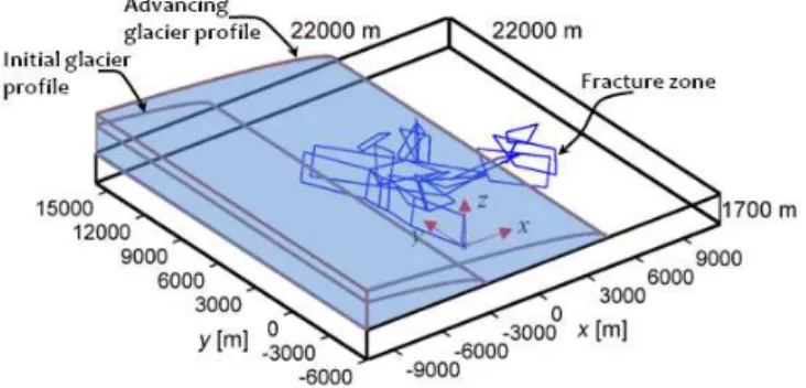
Figure 1.Geometry of the fractured rock mass subjected to loading by the advancing glacier.

solved with the COMSOL Multiphysics® finite element pro-gram. The equilibrium Eq. (5) is solved using the Structural Mechanics Module of the program; the fluid flow Eq. (6) is solved using the Earth Science Module (Darcy’s law); and the heat conduction Eq. (7) is solved using the Heat Trans-fer Module. By default these Modules are uncoupled, but the user can connect them by adding additional terms to the ap-propriate equations of each module as suggested by Eqs. (5) and (6).

2.2 The initial boundary value problem

Glacial loads on the surface of a rock mass arise due to the accumulation of snow, ice and water (Aschwanden and Blat-ter, 2009). The water content within a glacier is generally small (approximately 5 g of water per 1 kg of mixture) and the highest water content is found in the vicinity of the inter-face with the bedrock. The pattern of fluid flow both within and at the base of a glacier can be a complex THM process by itself. Problems associated with the mechanics of glaciers (Weertman, 1972; Marshall, 2005), the motion of glaciers (Fowler, 1981, 2011; Morland, 1987; Picasso et al., 2004; Gomez et al., 2013; Stucki and Schlunegger, 2013; Ahlkrona et al., 2013; Thoma et al., 2014), the constitutive properties of ice and ice-rock interfaces (Picasso et al., 2004; Marshall, 2005; Headley et al., 2012; Tezaur et al., 2015), the contact with the bedrock and the evolution of their shapes (dell’Isola and Hutter, 1998; Picasso et al., 2004; Dietrich et al., 2010; Headley et al., 2012; Nielsen et al., 2012; Pollard and de-Conto, 2012; Gomez et al., 2013; Stucki and Schlunegger, 2013; Steffen et al., 2006; de Boer et al., 2014) have been studied. The glacier dynamics on a centennial timescale due to climatic warming was studied by Hambrey et al. (2005).

Consider a model of a rock mass in the form of a par-allelepiped with upper surface z=ztop and lower surface z=zbot. Assume that a glacier of a non-uniform thickness moves along the upper surface of the rock,z=ztop, parallel to the (x, y) plane. The thickness of the glacier is denoted byH=H (x, y, t ), where(x, y)are the in-plane coordinates fixed at the base of the rock mass, as indicated in Fig. 1. As an

approximation of the complex shape of the glacier, the pro-file of the glacier is often considered to be parabolic (Chan and Stanchell, 2005; Chan et al., 2005; Steffen et al., 2014). In this case, the maximum ice-sheet thickness is expected to occur at the glacier centre and zero thickness at the glacier front. At the same time, it should be noted that the parabolic profile is very steep near the glacier front and very flat at the centre.

In order to examine the response of a poroelastic rock mass subjected to glacial loads, it is important to adequately take into account the interaction of the glacier with the underlying bedrock. On the temporal scale of interest to the glacial load-ing of a rock mass containload-ing fracture zones, a simpler rep-resentation of the glacier can be adopted. Firstly, mechanical loading due to the weight of the ice sheet needs to be pre-scribed (Bangtsson and Lund, 2008; Read, 2008). The me-chanical loading corresponds to the changing ice-sheet thick-nessH (x, y, t )and is applied as a time- and space-varying normal stress at the upper surface of the rock mass (Chan et al., 2005; Chan and Stanchell, 2008; Read, 2008; Steffen et al., 2006; Person et al., 2012; Pollard and deConto, 2012). Since the densities of the glacier constituents, water and ice, are almost equal, the total normal stress acting on the upper surface due to the presence of the glacier is given by σzz(x, y, ztop, t )= −ρfgH (x, y, t ). (8) Secondly, hydraulic boundary conditions must be prescribed. Boulton et al. (1995), Boulton and Caban (1995), Chan et al. (2005) and Person et al. (2012) state that if the perme-ability of the underlying rock is sufficiently low to discharge all basal meltwater as groundwater alone, groundwater heads are approximately equal to the ice pressures and the effec-tive pressures are low. For example, Person et al. (2012) pre-scribed head boundary conditions on the upper surface of the sedimentary basin assuming that the head is equal to 90 % of the ice sheet elevation. In this study the intact rock is assumed to have a very low permeability and thus the fluid pressure acting on the upper surface can be approximated by

p(x, y, ztop, t )= −σzz(x, y, ztop, t )=ρfgH (x, y, t ). (9) Therefore, the effective stress exerted by the glacier on the upper surface of the rock mass can be evaluated from Eqs. (2) and (9) as

σ_zz′ (x, y, ztop, t )= −(1−α)ρfgH (x, y, t ) <0. (10) To account for thermal loading caused by the presence of the glacier, the temperature change can be prescribed on the upper surface as

T (x, y, ztop, t )=Tu(x, y, t ), (11)

whereTuis a prescribed function.

velocity and the heat flux:

u3=0, ∂p ∂z =0,

∂T

∂z =0, z=z

bot_{. (12)}

On the vertical perimeter edges of the rock model we impose zero displacement, fluid velocity, and heat flux in the direc-tion of the normal to the surface:

un=0,

∂p ∂n=0,

∂T

∂n =0, (13)

where∂/∂n=n∇is the derivative in the direction normal to a surface.

Initial fields within the rock mass correspond to the fields existing at the onset of glacier motion and thus should in-clude stresses due to the weight of the glacier at its initial po-sition, geostatic stresses, hydrostatic fluid pressure, the tem-perature distribution due to the geothermal heat flux, etc. In this work we focus our attention only on thechangein the response of the rock mass caused by a small glacier advance and thus zero initial conditions can be prescribed, if the prob-lem is linear.

3 Finite element modelling 3.1 Model geometry

Figure 1 shows geometry of the fractured rock mass model used in the present study. The region of the rock mass is a parallelepiped with in-plane dimensions 22 000 m×22 000 m and a thickness of 1700 m. The fracture network is located at the interior of the rock mass domain, remote from its bound-aries. The specific fracture network examined here contains a system of 21 planar fractures within a region of (approxi-mately) 11 550 m×10 200 m. Details of the fracture network are shown in Figs. 1, 2 and 10. Each dominant fracture has the shape of a prism or prismatoid. The thickness of each fracture is set to 10 m. This is a realistic size for a fracture; an example of a 10 m wide fracture zone situated in the Rhone Valley of the Alps, the Simplon normal fault, is given in the paper by Stucki and Schlunegger (2013). In the fracture net-work, 14 fractures are subvertical with a high dip angle (close to 90◦), and 7 fractures are subhorizontal with a low dip an-gle (close to 0◦_{). Among the 14 subvertical fractures, 13}

frac-tures span the entire thickness of the rock model. Fracfrac-tures that do not span the entire thickness of the rock (e.g. sub-horizontal) originate at the upper surface of the rock. The subhorizontal fractures are numbered from 1 to 7 in Fig. 10. Each fracture zone is defined by its surface which consti-tutes a planar quadrilateral formed by the four vertices lying in the same plane. To facilitate construction of the fracture surface, a 2-D workplane is constructed for each fracture. Orientation of the workplane is defined by specifying co-ordinates of the vector normal to the fracture surface. The

fracture contour is drawn in the workplane by specifying co-ordinates of the four vertices of the fracture surface, trans-formed to the local coordinate system of the workplane. Sub-sequently, the fracture surface is extruded at a distance equal to the thickness of the fracture zone (10 m), forming a 3-D prism. Then this prism is embedded into a specified place within the geometry of the rock.

If a fracture originates at the upper surface of the rock, the upper edge of the fracture zone is expected to coincide with the upper surface of the rock, which is horizontal. However, after the extrusion process described above, if the fracture zone is not strictly vertical, the upper edge of the fracture (being orthogonal to the fracture surface) will be inclined with respect to the horizontal surface of the rock. Such a con-figuration may cause problems later during mesh generation since the edge of the fracture lies too close to the surface of the rock. To correct this geometry, the fractures’ surfaces in their respective workplanes can be extended in such a way that, after extrusion and embedding, the fracture intersects the upper surface of the rock and extends beyond it. Then we simply cut off the portion of the fracture zone above the up-per surface of the rock by using, for example, the subtraction operation. Similar corrections can be performed with respect to other edges of fractures that lie too close to the lower sur-face of the rock or to the perimeter sursur-faces. It should be noted that the fracture obtained in this way is a prismatoid and no longer an extruded feature.

Typically, it is desirable to have the capability of inserting into the 3-D geometry as many fractures as possible. On the other hand, if the geometry becomes too complex, the mesh may not be generated. Problems with mesh generation may arise when (a) the fractures are not parallel, i.e. have various orientations in space, (b) the number of intersections between fractures is too large, (c) the distance between the neighbour-ing fractures is too small, i.e. they are too close to each other, and (d) the thickness of fractures is too small. These con-ditions naturally place a limit on the number and the type of fractures that can be successfully inserted. We succeeded in inserting only 21 fracture zones into the geometry of the given rock mass as shown in Fig. 1. The basal rigid stratum will have an influence on the THM processes that are inves-tigated. The depth of 1.7 km is chosen to conform to previ-ous studies conducted by Chan and Stanchell (2008) so that there is a basis for comparison. When appropriate comput-ing resources are available, the extent of the domain can of course be increased to accommodate depths similar to those employed by Ustazewski et al. (2008) when examining com-posite faults in the Swiss Alps formed by the interplay of tec-tonics, gravitation and postglacial rebound occurring at depth regimes of up to 5 km.

3.2 Mesh generation

tetrahedral elements can be used and by default the or-der of the elements is quadratic. There are several pre-defined element sizes such as “Extremely Coarse”, “Extra Coarse”, “Coarser”, “Coarse”, “Normal”, “Fine”, “Finer”, “Extra Fine”, “Extremely Fine” and, in addition, the user can define the element size, “Custom” mesh size. Each mesh is characterized by the following parameters: maxi-mum element size, minimaxi-mum element size, maximaxi-mum ele-ment growth, resolution of curvature and resolution of nar-row regions. The values of these parameters are geometry-dependent. For example, for the given geometry of the rock mass, a parallelepiped with in-plane dimensions of 22 km×

22 km and a thickness of 1.7 km, the “Normal” mesh pa-rameters have the following values: maximum element size 2290 m, minimum element size 412 m, maximum element growth 1.5, resolution of curvature 0.6, resolution of narrow regions 0.5.

If the model geometry is too complex, it might be impos-sible to construct the mesh with the predefined mesh size due to the error messages. For example, for the present geometry of the fractured rock mass, COMSOL Multiphysics® failed to construct the “Normal” mesh, but managed to construct the “Extra Fine” mesh consisting of 3 321 534 elements and a “Fine” mesh with 223 530 elements. To reduce the num-ber of elements even further we define the “Custom” mesh size for which we assign the following values to the parame-ters: maximum element size 1690 m, minimum element size 172 m, maximum element growth 1.6, resolution of curvature 0.7, resolution of narrow regions 0.5. The resulting mesh has 158 728 tetrahedral elements and is shown in Fig. 2.

If the error message appears during mesh generation, it is recommended that the mesh size parameters be modified; even a small change in a parameter value can sometimes al-low COMSOL Multiphysics® to successfully construct the mesh. For example, for the given geometry with 21 fractures, one could construct the “Custom” mesh if the minimum ele-ment size is set to 152–154, 157, 159, 161, 167, 168, 170, 172, 186 or 189 m in the range of all values from 152 to 192 m. Otherwise, a change in the geometry should be at-tempted, such as deletion of the fracture that caused the error or a small translation of this fracture in the x–y plane. For example, deletion of the sub-horizontal fracture 2, marked in Fig. 10, extends the list of minimum element sizes for which the “Custom” mesh can be constructed to: 152–154, 157, 160, 161, 163, 164, 168, 170, 172, 173, 175, 177, 178, 180, 189 or 190 in the same range from 152 to 192 m. We note that even if a certain fracture was removed from the model due to the error messages, another fracture can still be inserted.

3.3 Glacial loading

The primary emphasis of this work is to examine the THM response of the fractured rock mass when it is subjected to advancing glacial loads. In general, advance or retreat of the

Figure 2.Finite element discretization of the rock mass with a sys-tem of interconnecting fracture zones. A discretization of 158 728 tetrahedral elements is used.

glacier can be caused by (a) sliding of the glacier along the bedrock and (b) a change in the accumulation and/or abla-tion rates. In the first case the shape of the glacier does not change, while in the latter case the shape of the glacier, i.e. its length and height, evolves. In the following we consider the glacier advance caused only by sliding, i.e. case (a).

Figure 1 shows the glacier profile at timet=0 and at time t >0, after the glacier has moved a distance of 7500 m paral-lel to thexaxis. The glacier front is assumed to be parallel to theyaxis. Initially, at timet=0, the glacier partially covers the model domain over the length of 7500 m; its front is lo-cated atx= −3159 m (Figs. 1, 3). It should be noted that the total glacier length is much larger than depicted in Fig. 1 but here only the marginal zone of the glacier that falls within the relatively small (compared to glacier length) dimensions of the model domain is shown.

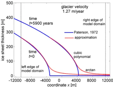
The thickness of the glacier is non-uniform and can be described by the functionH (X, t ), whereX is the distance from the centre of the glacier (datum point). LetHmax the maximum thickness of the glacier (at the centre), and L be the glacier length, i.e. distance from the glacier centre to its front. Then the functionH (X)at timet=0 satisfies H (0)=HmaxandH (L)=0. The specific form of the func-tionH (X, t )adopted from the paper by Paterson (1972) is shown in Fig. 3 and described in Appendix A. The max-imum glacier thickness is set equal toHmax=3200 m and H_max2 /L=7.7, which gives the lengthL=1 329 870 m. The profile of the ice sheet, shown in Fig. 3, is similar to that shown in Fig. 6 of the paper by Boulton and Caban (1995), in which, at a distance of 4000 m from the ice sheet front, the glacier thickness becomes equal to 300 m. Thex coordinate of the model domain, shown in Figs. 1 and 3, and the glacier Xcoordinate are related byx=X−1333029 m. The model domain boundaries are shown in Fig. 3 with vertical dashed lines.

The velocity of the glacierV is assumed to be 4.0306×

glacier velocity is about 100 times smaller than the one used by Chan et al. (2005) and about 10 times smaller than the velocity calculated by Aschwanden and Blatter (2009). Such a small glacier velocity is chosen to avoid problems with a loss of accuracy of the solution, which arise when the glacier velocity becomes higher and the mesh is not sufficiently fine (see Sect. 4.1). In addition to the actual glacier profile, shown with a solid line, Fig. 3 shows an approximation to this pro-file with a dashed line. This approximation coincides with the actual glacier profile away from the ice sheet front; how-ever, close to the leading edge of the ice sheet it replaces the actual profile with a much smoother function. In actual numerical computations, the use of this approximation is ad-vantageous since it does not have any sharp corners; smooth-ing the loadsmooth-ing profile has an extremely favourable effect on the convergence properties of the computational scheme, es-pecially when using iterative solvers.

As mentioned, the initial or in situ state is not modelled in the present study and therefore the loading applied to the surface of the rock mass only corresponds to the difference between the current position of the glacier, at timet, and its initial position att=0. (This is an admissible simplification of the problem when the problem is linear.) In this case, the maximum glacier loading will always be applied at the initial position of the glacier front; the amount of the glacier loading will decrease away from the initial positioning of the leading edge.

In the following we focus our attention on the response of the rock mass over a short time (e.g. 5900 years), for a small glacier advance, when the glacier front is still close to the fractured region of the rock and the glacier centre remains at a very large distance from the fractured region. Thus, we do not compute the results corresponding to the maximum value of the glacier loads, when the glacier centre itself overruns the model domain. The choice of the time frame can be ex-plained by the highly non-uniform distribution of the glacier load near the front of the glacier; our intention is to study the effect of this non-uniform load. In addition, we believe that the glacial sliding is limited to small distances compared to the overall glacier length.

3.4 Finite element solver

The response of the rock mass was obtained by using the transient finite element (FE) solver in COMSOL Multi-physics®. The numerical integration in time was implicit by default, which implies that a matrix factorization is required at each time step. Selecting the proper FE solver is of outmost importance because of the size of memory required, compu-tational time limitations and issues related to convergence. In order to solve the HM problem (Eqs. 5–6) for the “Cus-tom” mesh, a direct solver, such as the SPOOLES (SParse Object Oriented Linear Equations Solver) solver, requires a very large memory (larger than 30 GB) and a significant amount of time for matrix factorization. Thus, a direct solver

Figure 3. Distribution of the glacier thickness in the ice sheet marginal zone. The exact glacier shape is shown with a solid line and the approximation to the exact shape, used in the computational simulations, is shown with a dashed line.

cannot be used for the present problem. After testing sev-eral iterative solvers available in COMSOL Multiphysics®, it was found that the iterative GMRES (Generalized Minimal RESidual method) solver with the geometric multigrid pre-conditioner was, in fact, the only solver capable of dealing with this problem within a reasonable time frame (approx-imately 3 h of runtime when solving the HM problem and 8 h for the THM problem). On the memory side, GMRES required only slightly more than 6 GB of RAM. Other pre-conditioners had slower runtimes due to convergence issues. 3.5 Material properties

The fracture zones have THM properties substantially differ-ent from those of the intact rock. In particular, the perme-ability of the fracture zones is taken to be about six orders of magnitude greater than the permeability of the intact rock, whereas Young’s modulus is assumed to be approximately 10 times smaller.

The properties of the intact rock and the fractures used in our computational simulations are the following: Young’s modulusED is 30 GPa for the intact rock and 3 GPa for the fractures; Poisson’s ratioνD is 0.25; the Biot coefficientα is 0.7; permeabilityk is 1.55×10−19m2for the intact rock and 3×10−13m2for the fractures; dynamic viscosity µis 0.001 Pa s; fluid bulk modulusKfis 2.2 GPa; thermal expan-sion coefficient for the solid phaseαsis 8.3×10−61/◦C and for the fluid phaseαfis 69×10−61/◦C; equivalent specific heatcpis 1.8305×106N/(m2K); and equivalent

used by Chan and Stanchell (2008) to model the Canadian Shield subregion. Alterations to fracture permeabilities dur-ing glacial loaddur-ings are important but these extensions are not considered in this study. The estimation of the permeability of fractures in particular is governed by the hydraulic aper-ture of the fracaper-ture, which can be influenced by the normal and shear stresses acting on the fracture and gouge develop-ment (Nguyen and Selvadurai, 1998; Selvadurai and Nguyen, 1999; Selvadurai and Yu, 2005; Selvadurai, 2015). Discus-sions of these topics and references to further studies of this important topic are given by Boulon et al. (1993), Nguyen and Selvadurai (1998) and Selvadurai (2015).

4 Model performance

In this section we assess our choice of the user-defined “Custom” mesh, consisting of 158 728 tetrahedral elements (Fig. 2), and show that this mesh is suitable for solving the given problem of the bedrock response if the glacier speed is as low as 1.27 m year−1. We will refer to this “Custom” mesh as “fracture-biased” mesh.

4.1 Mesh refinement evaluation for homogeneous rock The first evaluation procedure involves analysis of the HM solutions for the homogeneous rock, i.e. the rock in which properties of the fractures are the same as those of the in-tact part. Here we examine how the presence of the densely refined regions in the mesh, in close proximity to the “frac-ture” zones, may affect the solution. To do so, in addition to the “Custom” mesh we consider the regular mesh with only 5786 elements that does not account for the presence of “fracture” zones.

Figure 4 shows the distribution of vertical fluid velocity vz in the homogeneous rock for the two meshes described

above. The time is 5900 years, during which time the glacier has moved a distance of 7500 m. The current position of the glacier front corresponds to transitioning from negative to positive velocity values, which is clearly seen in the figure. The magnitude of the negative velocity is considerably larger than the positive velocity. It can be seen that the fluid veloc-ity distributions for the two meshes are quite similar, i.e. the presence of densely-meshed fracture zones does not change the solution significantly. This is an expected result since the rock is homogeneous. Our numerical tests also showed that the solution for the “Custom” fracture-biased mesh deviates significantly from the regular solution once the glacier speed is increased to 12.7 m year−1. This implies that for a larger glacier velocity, the finer mesh will be required.

4.2 Mesh refinement evaluation for the hydraulic problem

The second evaluation procedure employed involves a com-parison of the solutions for two meshes: the user-defined

Figure 4.Vertical fluid velocity [m s−1] in the homogeneous rock for the fracture-biased mesh with 158 728 elements (top) and for the regular mesh with 5786 elements (bottom). Time is 5900 years and glacier velocity is 1.27 m year−1.

“Custom” mesh with 158 728 elements and the pre-defined “Extra Fine” mesh with 3 321 534 elements. Taking into ac-count the fact that the “Extra fine” mesh has a massive num-ber of elements, which would require a considerable amount of memory, we could solve only the “pure” hydraulic prob-lem (Eq. 6) in which the deformations of the porous skeleton are suppressed, thus reducing the number of unknowns.

Figure 5 shows the distribution of vertical fluid velocityvz

Figure 5. Vertical fluid velocity [m s−1] in the intact part of the fractured rock for “Custom” mesh (top) and “Extra Fine” mesh (bot-tom). Time is 5900 years and glacier velocity is 1.27 m year−1. The velocity is obtained by solving a pure hydraulic problem.

5 Numerical example

5.1 Solution of HM problem for “Custom” mesh Figures 6–15 show the hydro-mechanical response of the fractured rock subjected to glacial loading, described pre-viously, at time 5900 years. The time-dependent fluid pres-sure and vertical compressive stress induced by the glacial load are applied to the upper surface of the rock mass as pre-scribed by Eqs. (8) and (9). The solution is obtained by solv-ing the hydro-mechanical problem (Eqs. 5, 6) on the user-defined “Custom” mesh. For more accurate results, the model domain, shown in Figs. 1 and 2, was augmented along the x axis by two blocks of 22 000 m length each behind the glacier front, and by one block of 14 000 m length ahead of the glacier front. The total length of the augmented do-main is therefore 80 000 m, while the size along they axis remains the same at 22 000 m. Mesh size parameters retain

the same values as for the user-defined “Custom” mesh, described above. The new blocks are fracture-free and are discretized using regular, non-biased meshes. The resulting mesh for the extended domain has 167 303 tetrahedral ele-ments, just slightly more than the fracture-biased mesh for the main block of the domain, containing fractures. The in-creased length of the model domain enables us to take into account the glacier loading more accurately.

Figure 6 shows the typical fluid pressure distribution at the interior, fractured region of the rock and exterior, ho-mogeneous region at time 5900 years. To capture the re-sponse in the fractured region, the fluid pressure was plot-ted in the cross section where the y coordinate was equal to 6200 m, which is approximately at the mid-section of the rock mass (see Fig. 1). As is expected, the fluid pressure close to the lower surface is generally smaller than the pressure ap-plied at the upper surface. The maximum fluid pressure oc-curs close to the initial location of the ice sheet front, i.e. tox= −3159 m. Within and around the fractures, the fluid pressure is almost uniform through the thickness as the sure induced at the lower surface is almost equal to the pres-sure applied at the upper surface. Such a response is caused by the high permeability of the fractures. However, away from the fracture zones, the pressure at the lower surface re-mains smaller than that at the upper surface, due to the low permeability of the intact rock. This pressure difference cre-ates a vertical pressure gradient∂p/∂zand a fluid flow in the downward direction. For the purpose of comparison, Fig. 6 also shows the distribution of fluid pressure in the homoge-neous region of the rock in a cross section parallel to the xaxis; the influence of the fractures in altering the fluid pres-sure distribution in the region due to glacier loading is quite evident. In particular, we can observe that the pressure in the intact rock in close proximity to the fractures is larger than the pressure in the fracture-free, or homogeneous, region of the rock, for the same value of thex coordinate. This im-plies that the vertical fluid velocity in the intact rock near the fractures is generally expected to be smaller than that in the homogeneous region of the rock (see also Figs. 7 and 8).

Figure 6. Distribution of fluid pressure [Pa] in the fractured and homogeneous regions of the rock in cross sections y=const at time 5900 years. For the fractured regiony=6200 m. The rock is subjected to spatially non-uniform fluid pressure and compressive stress.

Figure 7.Variation of fluid pressure [Pa] in the cross sections of the fractured and homogeneous regions of the rock;y=6200 and −3200 m, respectively, at a depth of 200 m and at time 5900 years. The rock is subjected to spatially non-uniform fluid pressure and compressive stress.

Figure 8 shows the vertical fluid velocity vz in the

in-tact part of the rock with fracture zones at time 5900 years. The vertical velocity distribution in the rock is complex. The fluid velocity can be both positive and negative. A nega-tive fluid velocity implies that fluid flow takes place into the rock (i.e. downwards) and a positive fluid velocity implies that the fluid flows out of the rock (i.e. upwards). It can be seen that, in general, the magnitude of the negative veloc-ity is much larger than the positive velocveloc-ity, which is con-sistent with the direction of the meltwater flow. In fact, be-neath the glacier most of the fluid flows into the rock with a velocity of −3×10−13m s−1 and, exterior to the glacial

Figure 8.Distribution of the vertical fluid velocity [m s−1] in the intact part of the rock mass with fracture zones at time 5900 years. The rock mass is subjected to spatially non-uniform fluid pressure and compressive stress imposed by the advancing glacier.

footprint, most of the fluid flows out of the rock with a veloc-ity 2.5×10−14m s−1. Between the fractures the magnitude of the negative fluid velocity in the intact rock is in general smaller compared to that in the homogeneous region of the rock (as the dark blue colour in the exterior region of the rock changes to light blue, yellow and even red in the interior re-gion at close proximity to the fractures).

Figure 9 shows variation of the vertical fluid velocity in the intact part of the rock mass with fractures in the cross sectionsy=6200 and−3200 m corresponding to the frac-tured and homogeneous regions, respectively, at a depth of 200 m from the upper surface, at time 5900 years. The fig-ure clearly shows how the presence of fractfig-ures affects the fluid velocity in the intact rock near the fractures: the fluid velocity in the intact rock of the fractured region is smaller, in absolute value, than the velocity in the fracture-free region of the rock.

Figure 10 illustrates the vertical fluid velocityvzwithin the

fractures of the rock at 5900 years. It can be seen that in the fractures oriented subvertically (most fractures are subverti-cal) the fluid velocity is much larger than that in the intact part of the rock (compare Fig. 10 with Fig. 8). In fact, the maximum fluid velocity in the fractures can reach a value of

Figure 9. Vertical fluid velocity [m s−1] in the intact part of the rock mass with fracture zones for the cross sectionsy=6200 and −3200 m in the fractured and homogeneous regions, respectively, at a depth of 200 m and at time 5900 years.

Figure 10.Distribution of the vertical fluid velocity [m s−1] within the fracture zones at time 5900 years. The rock mass is subjected to spatially non-uniform fluid pressure and compressive stress im-posed by the advancing glacier. Subhorizontal fractures are num-bered 1–7.

the vertical fluid velocity is towards the upper surface of the rock and can reach the value of+5×10−8m s−1_{, although} this fracture is totally covered by the glacier at 5900 years. The fact that some fluid in the fracture can flow towards the upper surface can be explained by the non-uniform distribu-tion of the ice sheet loading along the x axis and the very high permeability of fractures. It should also be noted that in the fractures with a low dip angle (subhorizontal orientation) the vertical fluid velocity is generally smaller than that in the subvertical fractures.

Figure 11 shows variation of the vertical fluid velocity in the largest fracture zone along its length, at a depth of 200 m

Figure 11.Variation of the vertical fluid velocity [m s−1] in the largest fracture zone, at a depth of 200 m and at time 5900 years. Velocity is approximately uniform across the fracture’s thickness.

Figure 12.Vertical displacement [m] of the rock mass with frac-tures at time 5900 years. The rock is subjected to spatially non-uniform fluid pressure and compressive stress.

from the upper surface, at time 5900 years. At this depth the velocity distribution is approximately uniform across the thickness of the fracture. It is apparent from the figure that at this depth the velocity in the fracture remains high and nega-tive at one end of the fracture (−3×10−8m s−1) and positive at another end (+5×10−8m s−1).

Figure 13.Variation of the vertical displacement [m] in the rock mass with fractures in the cross sectionsy=6200 and −3200 m corresponding to the fractured and homogeneous regions respec-tively and at a depth of 200 m, at time 5900 years.

Selvadurai and Nguyen, 1995). The maximum negative dis-placement (−0.076 m) is near the front of the glacier at its initial position. It can be observed that the displacements in the fractured and homogeneous regions of the rock are not very different, i.e. the displacement field is not strongly in-fluenced by the presence of fractures with low deformability properties.

Figure 13 shows variation of the vertical displacement in the rock mass with fracture zones in the cross sections of the fractured and fracture-free regionsy=6200 and −3200 m, respectively, at a depth of 200 m below the upper surface, at time 5900 years. The vertical displacement is in fact smaller, in absolute value, in the fractured region of the rock although the difference between the displacements in the fractured and fracture-free regions of the rock is not significant.

Figure 14 shows the mean effective stress (σ_xx′ +σ_yy′ + σ_zz′ )/3 in the intact part of the rock with fractures at 5900 years. The mean effective stress is mostly compres-sive but tensile stresses do occur in the fractured region at the upper surface (dark red patch). The maximum compres-sive stress occurs near the lower surface of the rock close to the initial location of the ice sheet front. The distinctive feature of the response of the rock with fractures is the exis-tence of tensile stresses near the upper surface between and around the fractures (dark red patch); however, the magni-tude of these tensile stresses is smaller than the compressive stress. It can also be observed that in the homogeneous, ex-terior region of the rock, the stress is entirely compressive. It should be noted that for any failure analysis the HM stress state resulting from glacial loading should be combined with the in situ geostatic stress, GIA stress (Steffen et al., 2006) and possible tectonic background stresses.

Figure 14.Distribution of the mean effective stress [Pa] within the intact part of the rock mass with fracture zones at time 5900 years. The rock is subjected to spatially non-uniform fluid pressure and compressive stress.

Figure 15.Variation of the mean effective stress [Pa] in the intact part of the rock mass with fracture zones in the cross sections of the fractured and homogeneous regions of the rock massy=6200 and −3200 m respectively, at a depth of 200 m and at time 5900 years.

5.2 Solution of THM problem for “Custom” mesh In the thermo-hydro-mechanical problem the temperature change caused by glacier advance or growth must be pre-scribed at the upper surface of the rock. Chan et al. (2005) ex-amined the change in the ground surface temperature through the entire glacial cycle using climate/temperature simulation. From this simulation it was clear that before the arrival of the glacier, the ground surface temperature decreases signif-icantly from +10 to −25◦C. As the glacier gradually oc-cupies the domain of interest, the insulating effect of the ice sheet gradually increases the subglacial temperature from

−25 to 0◦C. This complex temperature evolution at the up-per surface of the rock mass is simplified in the present work and only a net cool down from+10 to 0◦_{C, associated with}

the glaciation period, is considered. Similar surface temper-ature evolution was used in the study by Read (2008): the mean annual surface temperature was set to +7◦C during non-glacial periods and, to account for glaciation, the mean annual rock mass surface temperature was reduced to 0◦C.

In Figs. 16–19 we illustrate the response of the rock mass with fracture zones subjected to the glacial load described previously and, in addition, to the effects of cooling asso-ciated with the advance of the glacier. The time-dependent fluid pressure, the vertical compressive stress and the tem-perature change are applied to the upper surface of the rock mass as prescribed by Eqs. (8), (9) and (11). As indicated previously, the initial or in situ state is not taken into account in the present study and, therefore, only the surface loading and temperature that correspond to the difference between the current position of the glacier, at time t, and its initial position are applied to the surface of the rock. The tempera-ture change on the upper surface caused by glacier advance is assumed to have the following form:

1T (x, y, ztop, t )=Tmax

_{H (x, t )}

Hmax

−H (x,0) Hmax

, (14)

whereH (x, t ) is the smoothed/approximated glacier thick-ness at time t (Appendix A). The maximum temperature change is set equal to Tmax= −10◦C and will be reached at the initial location of the ice sheet front whent=L/V=

1 047 000 years, i.e. when the centre of the glacier over-runs the model domain. Since in this study attention is re-stricted only to a small glacier advance, this time can never be reached during computational simulations, i.e. the glacier motion will be terminated a long time before this time is reached.

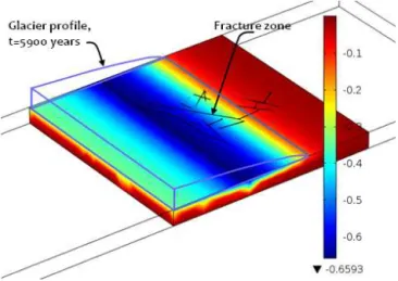
Figure 16 shows the temperature change generated within the rock 5900 years after initiation of the glacier motion. The temperature change on the upper surface is prescribed according to Eq. (14). The temperature change under the glacier reaches the maximum of−0.66◦C at the upper sur-face of the rock close to the initial location of the ice sheet front and is almost zero beyond the glacier margin. (The cur-rent maximum of −0.66◦C is much smaller than Tmax=

Figure 16.Temperature change distribution [◦C] within the rock mass 5900 years after the start of the glacier advance.

−10◦C since the centre of the glacier is very far from the model domain boundaries at time 5900 years.) We observe that the distribution of the temperature through the thickness of the rock mass under the glacier is non-uniform, which im-plies that the temperature did not reach the steady state in 5900 years and at the lower surface of the rock the tempera-ture is still above the value prescribed at the upper surface.

Figure 17 shows the variation of the temperature change at the upper surface of the rock mass and at a depth of 800 m from the upper surface, at time 5900 years. The dependence of the temperature field on they coordinate is only due to a difference in the mesh refinement in the fractured and ho-mogeneous regions and thus rather weak. From the figure it is evident that the temperature at a depth of 800 m is much smaller than the prescribed temperature at the upper surface, which suggests that even for such a small glacier speed a steady state was not reached in 5900 years.

Figure 18 shows the mean effective stress in the intact part of the rock with fractures at time 5900 years. The rock mass is subjected to the compressive stress, the fluid pressure in-duced by the glacial load and the temperature field (Eq. 14) associated with the glacial advance. We note that the com-pressive mean stress at the lower surface of the rock mass is almost equal to that in the rock subjected only to the mechan-ical load and fluid pressure (see Fig. 14). However, the tensile mean stress, which occurs in the fractured region in the vicin-ity of the upper surface, is increased from 0.15 to 0.28 MPa. In contrast to the effective stress, the vertical fluid velocity is not significantly influenced by the cooling; the velocity field in the rock subjected to the compressive stress, the fluid pres-sure and the temperature field (Eq. 14) is almost the same as that in the rock subjected only to the mechanical load and fluid pressure (as shown in Figs. 8 and 9).

Figure 17.Temperature change [◦C] in the rock mass at the upper surface and at a depth of 800 m and at time 5900 years.

Figure 18.Distribution of the mean effective stress [Pa] within the intact part of the rock mass with fracture zones at time 5900 years. The rock is subjected to spatially non-uniform fluid pressure, com-pressive stress state and temperature change.

through the fractured and fracture-free regionsy=6200 and

−3200 m, respectively, at time 5900 years. At this depth the mean effective stress in the rock of the fracture-free region is compressive, approximately equal to−0.15 MPa, whereas the stress in the intact rock of the fractured region remains tensile, reaching the value of+0.15 MPa.

6 Concluding remarks

In the present work, the behaviour of a fractured rock mass subjected to advancing glacial loads was analysed. The glacial load was taken into account by prescribing a spa-tially and time-dependent compressive stress and fluid

pres-Figure 19.Variation of the mean effective stress [Pa] in the in-tact part of the rock mass with fracture zones in the cross sec-tionsy=6200 and−3200 m, corresponding to the fractured and homogeneous regions, respectively, at a depth of 200 m and at time 5900 years.

sure on the upper surface of the rock mass. Resulting fluid pressures, vertical fluid velocities, displacements, and mean stress distribution diagrams were obtained through computa-tional simulations that incorporated THM processes. Results were plotted for the specific time of 5900 years during which the glacier advanced across the model domain by a distance of approximately 7500 m.

The computational results show that there is a difference between the fluid pressures at the upper and lower surfaces of the rock mass due to the low permeability of the intact rock. This pressure difference creates a vertical pressure gra-dient that contributes to the vertical fluid velocity compo-nent, which is a major feature of the fluid flow in the present problem. We also observed a difference in the fluid pressure distributions within the fractured region and the surrounding homogeneous region of the rock. In fact, the fluid pressure within the fracture zones and the intact rock in close prox-imity to the fractures is larger than that in the homogeneous region, located remotely from the fracture zones. This can be attributed to the large permeability of the fractures.

times larger than the velocity in the intact rock. The direc-tion of the fluid velocity in the fractures is mainly negative but large velocities in the positive direction can also occur, especially in the subvertical fractures that are not parallel to the ice sheet front. The role of the fracture zones and their dominant influence on the fluid flow in the region during a glaciation event is thus confirmed by the present study.

The mean effective stress in the intact part of the rock mass is mostly compressive, but tensile stresses do occur between and around the fractures, at close proximity to the upper sur-face of the rock. The maximum compressive stress is at the lower surface of the rock at the initial position of the ice sheet front. The glacial loading induces compression of the rock, i.e. negative strain in the direction of the rock thickness. For the situations examined in the paper, this axial compression is relatively uninfluenced by the presence of fracture zones. In addition to the compressive stress and fluid pressure, the given rock mass was subjected to the cooling associated with a glacier advance. Since the present study considers a small glacier advance of only 7500 m, the associated temperature change is also small, only −0.66◦C. It was observed that even for this small temperature change, the mean effective tensile stress noticeably increases at the upper surface of the rock between and around the fractures. However, the effect of the cooling on the vertical fluid velocity distribution in the fractured rock was small. These results suggest that the hydro-thermal interaction in the present problem can be ne-glected, but the effect of cooling on the stress distribution in the intact part of the rock (thermo-mechanical interaction) should be given greater consideration.

This study is closely related to the work performed earlier by Chan et al. (2005) and Chan and Stanchell (2005, 2008) in that it also examines the effect of the glacial loading on the behaviour of fractured bedrock. In their work the rock was modelled as a thermo-poroelastic medium and contained 3-D (but narrow) fracture regions, which were also assumed thermo-poroelastic. The novelty of the present model is the use of a quite complicated fracture network consisting of 21 fractures whereas only 5 fractures were included into the

models described in the papers by Chan et al. (2005) and Chan and Stanchell (2005). The NWMO report by Chan and Stanchell (2008) deals with a more complex fracture network consisting of 19 fractures but the fracture thickness is set to 20 m, whereas in the present work it is 10 m, which implies greater geometry and mesh complexity. In addition, in the present study the focus is on the transient response caused by highly non-uniform and moving glacial loading acting on the surface of the bedrock. This loading is directly linked to the specified glacier velocity and profile. Another novelty of this work is the investigation of the use of a commercially available finite element code, which can reduce the efforts of the users in solving the present problem by finite element method.

Appendix A

The initial position of the glacier can be described by the functionH (X), whereH is the thickness of the glacier and X is the distance from the centre of the glacier (the da-tum point). The function H (X)satisfies H (0)=Hmaxand H (L)=0, whereHmaxis maximum thickness of the glacier andLis the distance from the centre to the glacier front.

The glacier has accumulation and ablation zones. For sim-plicity, we assume that the net thickness of ice added to the surface each year in the accumulation zone is equal to the net thickness of the ice lost each year in the ablation zone. Ow-ing to this assumption, the accumulation and ablation zones have equal lengths,L/2. In this case, the profile of the glacier in the steady state can be obtained as (Paterson, 1972)

H (X)=21/8Hmax

_L−X L

1/2 ,

in the ablation zoneL/2< X < L; _{H (X)}

Hmax

8/3 +21/3

_X

L 4/3

=1,

in the accumulation zone 0< X < L/2. (A1) Knowing the velocity of the ice sheetV and the initial pro-file, given by (A1), we can obtain the equation for the glacier profile in the ablation zone as a function of time:

H (X, t )=21/8Hmax

_{L−X+V t} L

1/2 ,

in the ablation zoneL/2< X−V t < L. (A2) The approximation to the parabolic profile (Eq. A2) is evalu-ated by the formula

H (x, t )=21/8Hmax

_−x[

m] −3159+V t L

1/2 ,

x−V t≤ −10 759 m;

H (x, t )=A3(x−V t )3+A2(x−V t )2+A1(x−V t )+A0,

−10 759≤x−V t≤ −3759 m; H (x, t )=200F (x, t ), x−V t≥ −3759 m;

F (x, t )=1

2+ 1 πarctan

1

1200(−x[m] −4159+V t )

.

Code availability

The source files used in the computations performed in connection with this paper can be found at the follow-ing links: https://www.dropbox.com/s/83b1gcrukw47sib/ glacierproblem_mesh158728_noheat.mph?dl=0, https: //www.dropbox.com/s/oy7fo28303td1lf/glacierproblem_ mesh158728_withheat.mph?dl=0.

Acknowledgements. The work described in this paper was initiated through the research support provided by the Nuclear Waste Man-agement Organization, Ontario, and through a Discovery research grant awarded to A. P. S. Selvadurai by the Natural Sciences and Engineering Research Council (NSERC) of Canada. A co-author (P. A. Selvadurai) is grateful to NSERC for a post-graduate scholarship, which enabled him to participate in the research. The opinions expressed in the paper are those of the authors and not of the research sponsors. The authors are grateful to the topical editor Lutz Gross and two anonymous reviewers for their valuable comments, which led to significant improvements in the presentation.

Disclaimer. The use of the computational code COMSOL Multiphysics® is for demonstrational purposes only. The authors neither advocate nor recommend the use of the code without conducting suitable evaluations to test the accuracy of the code in a rigorous fashion.

Edited by: L. Gross

References

Ahlkrona, J., Kirchner, N., and Lötstedt, P.: Accuracy of the zeroth- and second-order shallow-ice approximation – numeri-cal and theoretinumeri-cal results, Geosci. Model Dev., 6, 2135–2152, doi:10.5194/gmd-6-2135-2013, 2013.

Alonso, E. E., Alcoverro, J., Coste, F., Malinsky, L., Merrien-Soukatchoff, V., Kadin, I., Nowak, T., Shao, H., Nguyen, T. S., Selvadurai, A. P. S., Armand, G., Sobolik, S. R., Itamura, M., Stone, C. M., Webb, S. W., Rejeb, A., Tijani, M., Maouche, Z., Kobayashi, A., Kurikami, H., Ito, A., Sugita, Y., Chijimatsu, M., Borgesson, L., Hernelind, J., Rutqvist, J., Tsang, C.-F., and Jus-sila, P.: The FEBEX benchmark test: case definition and compar-ison of behavior approaches, Int. J. Rock Mech. Min. Sci., 42, 611–638, 2005.

Aschwanden, A. and Blatter, H.: Mathematical modeling and nu-merical simulation of polythermal glaciers. J. Geophys. Res. 114, F01027, doi:10.1029/2008JF001028, 2009.

Bangtsson, E. and Lund, B.: A comparison between two solution techniques to solve the equations of glacially induced deforma-tion of an elastic Earth, Int. J. Num. Meth. Eng., 75, 479–502, 2008.

Biot, M. A.: General theory of three-dimensional consolidation, J. Appl. Phys., 12, 155–164, 1941.

Booker, J. R. and Savvidou, C.: Consolidation around a point heat source, Int. J. Num. Anal. Meth. Geomech., 9, 173–184, 1985.

Boulon, M. J., Selvadurai, A. P. S., Benjelloun, H., and Feuga, B.: Influence of rock joint degradation on hydraulic conductivity, Int. J. Rock Mech. Min. Sci. Geomech. Abstr., 30, 1311–1317, 1993. Boulton, G. S. and Caban, P.: Groundwater flow beneath ice sheets: part II – its impact on glacier tectonic structures and moraine formation, Quat. Sci. Rev., 14, 563–587, 1995.

Boulton, G. S., Caban, P., and Gijssel, K.: Groundwater flow be-neath ice sheets: part I−large scale patterns, Quat. Sci. Rev., 14, 545–562, 1995.

Boulton, G. S., Chan, T., Christiansson, R., Ericsson, L., Jensen, M. R., Stanchell, F. W., and Wallroth, T.: Thermo-hydro-mechanical (T-H-M) impacts of glaciation and implications for deep geolog-ical disposal of nuclear waste, in: Geo-engineering Book Series, vol. 2. Coupled thermo-hydro-mechanical-chemical processes in geosystems, edited by: Stephansson, O., Hudson, J. A., and Jing, L., Elsevier Amsterdam, 299–304, 2004.

Chan, T. and Stanchell, F. W.: Subsurface hydro-mechanical (HM) impacts of glaciation: sensitivity to transient analysis, HM cou-pling, fracture zone connectivity and model dimensionality, Int. J. Rock Mech. Min. Sci., 42, 828–849, 2005.

Chan, T. and Stanchell, F. W.: DECOVALEX THMC TASK E – Im-plications of Glaciation and Coupled Thermo-hydro-mechanical Processes on Shield Flow System Evolution and Performance Assessment, NWMO TR-2008-03, Nuclear Waste Management Organization, Toronto, ON, Canada, 2008.

Chan, T., Christiansson, R., Boulton, G. S., Ericsson, L. O., Har-tikainen, J., Jensen, M. R., Mas Ivars, D., Stanchell, F. W., Vis-trand, P., and Wallroth, T.: DECOVALEX III BMT 3/BENCH-PAR WP4: The thermo-hydro-mechanical responses to a glacial cycle and their potential implications for deep geological dis-posal of nuclear fuel waste in a fractured crystalline rock mass, Int. J. Rock Mech. Min. Sci., 42, 805–827, 2005.

Chapman, N. A. and McKinley, I. G.: The Geological Disposal of Nuclear Waste, John Wiley, New York, 280 pp., 1987.

de Boer, B., Stocchi, P., and van de Wal, R. S. W.: A fully cou-pled 3-D ice-sheet–sea-level model: algorithm and applications, Geosci. Model Dev., 7, 2141–2156, doi:10.5194/gmd-7-2141-2014, 2014.

dell’Isola, F. and Hutter, K.: What are the dominant thermo-mechanical processes in the basal sediment layer of large ice sheets?, Proc. Roy. Soc. A Math Phys., 454, 1169–1195, 1998. Dickson, M. H. and Fanelli, M. (Eds.): Geothermal Energy, 224 pp.,

John Wiley, New York, 1995.

Dietrich, R., Ivins, E.R., Casassa, G., Lange, H., Wendt, J., and Fritsche, M.: Rapid crustal uplift in Patagonia due to enhanced ice loss, Earth Planet. Sci. Lett., 289, 22–29, 2010.

Erhel, J., De Dreuzy, J.-R., and Poirriez, B.: Flow simulation in three-dimensional discrete fracture networks, SIAM J. Sci. Com-put., 31, 2688–2705, 2009.

Fowler, A. C.: A theoretical treatment of the sliding of glaciers in the absence of cavitation, Phil. Trans. Roy. Soc. Lond., A407, 637–685, 1981.

Fowler, A. C.: Mathematical Geoscience, 902 pp., Springer-Verlag, Berlin, 2011.

Graf, T. and Therrien, R.: A method to discretize non-planar frac-tures for 3D subsurface flow and transport simulations, Int. J. Num. Meth. Fluids., 56, 2069–2090, 2008.

Guvanasen V. and Chan, T.: Three-dimensional numerical model for thermo-hydro-mechanical deformation with hysteresis in a fractured rock mass, Int. J. Rock Mech. Min. Sci., 37, 89–106, 2000.

Hambrey, M. J., Murray, T., Glasser, N.F., Hubbard, A., Hubbard, B., Stuart, G., Hansen, S., and Kohler, J.: Structure and chang-ing dynamics of a polythermal valley glacier on a centennial timescale: Midre Lovenbreen, Svalbard, J. Geophys. Res., 110, F01006, doi:10.1029/2004JF000128, 2005.

Hamiel, Y., Lyakhovsky, V., and Agnon, A.: Rock dilation, non-linear deformation, and pore pressure change under shear, Earth Planet. Sci. Lett., 237, 577–589, 2005.

Headley, R. M., Roe, G., and Hallet, B.: Glacier longitudinal pro-files in regions of active uplift, Earth Planet. Sci. Lett., 317, 354– 362, 2012.

Juanes, R., Samper, J., and Molinero, J.: A general and efficient formulation of fractures and boundary conditions in the finite el-ement method, Int. J. Num. Meth. Eng., 54, 1751–1774, 2002. Khalili, N. and Selvadurai, A. P. S.: A fully coupled constitutive

model for thermo-hydro-mechanical analysis in elastic media with double porosity, Geophys. Res. Lett., 30, SDE 7-1–7-5, 2003.

Lachenburch, A.: Friction heating, fluid pressure and the resistance to fault motion, J. Geophys. Res., 85, 6097–6112, 1980. Laughton, A. S., Roberts, L. E. J., Wilkinson, D., and Gray, D.

A. (Eds.): The Disposal of Long-Lived and Highly Radioac-tive Wastes, Proceedings of a Royal Society Discussion Meeting, Royal Society, London, 189 pp., 1986.

Marshall, S. J.: Recent advances in understanding ice sheet dynam-ics, Earth Planet. Sci. Lett., 240, 191–204, 2005.

Massart, T. J. and Selvadurai, A. P. S.: Stress-induced permeability evolution in a quasi-brittle geomaterial, J. Geophys. Res., 117, B07207, doi:10.1029/2012JB009251, 2012.

Massart, T. J. and Selvadurai, A. P. S.: Computational modelling of crack-induced permeability evolution in granite with dilatant cracks, Int. J. Rock Mech. Min. Sci., 70, 593–604, 2014. McNutt, M. and Menard, H. W.: Lithospheric flexure and uplifted

atolls, J. Geophys. Res., 83, 1206–1212, 1978.

McTigue, D. F.: Thermoelastic response of fluid-saturated porous rock, J. Geophys. Res., 91, 9533–9542, 1986.

Morland, L. W.: Unconfined ice-shelf flow, in: Ice Dynamics of the West Antarctica Ice sheet Vol. 4. Glaciology and Quaternary Ge-ology, edited by: van der Veen, C. J. and Oerlemans, J., Springer-Verlag, Berlin, 99–116, 1987.

Najari, M. and Selvadurai, A. P. S.: Thermo-hydro-mechanical re-sponse of granite to temperature changes, Env. Earth Sci., 72, 189–198, doi:10.1007/s12665-013-2945-3, 2014.

Ng, K. L. A. and Small, J. C.: Behavior of joints and interfaces subjected to water pressure, Comput. Geotech., 20, 71–93, 1997. Nguyen, T. S. and Selvadurai, A. P. S.: Coupled thermal-mechanical-hydrological behaviour of sparsely fractured rock: implications for nuclear fuel waste disposal, Int. J. Rock Mech. Min. Sci., 32, 465–479, 1995.

Nguyen, T. S. and Selvadurai, A. P. S.: A model for coupled me-chanical and hydraulic behaviour of a rock joint, Int. J. Num. Anal. Meth. Geomech., 22, 29–48, 1998.

Nguyen, T. S., Selvadurai, A. P. S., and Armand, G.: Modelling the FEBEX THM experiment using a state surface approach, Int. J. Rock Mech. Min. Sci., 42, 639–651, 2005.

Nielsen, K., Khan, S. A., Kosgaard, N. J., Kjær, K. H., Wahr, J., Bevis, M., Stearns, L. A., and Timm, L. H.: Crustal uplift due to ice mass variability on Upernavik Isstrøm, west Greenland, Earth Planet. Sci. Lett., 353/354, 182–189, 2012.

Noorishad, J., Tsang, C.-F., and Witherspoon, P. A.: Coupled thermo-hydraulic-mechanical phenomena in saturated fractured porous rocks: numerical approach, J. Geophys. Res., 89, 10365– 10373, 1984.

Paterson, W. S. B.: Laurentide ice sheet: estimated volumes during late Wisconsin, Rev. Geophys. Space Phys., 10, 885–917, 1972. Peltier, W. R.: Global glacial isostasy and the surface of the ice-age

earth: The ICE-5G (VM2) model and GRACE, Annu. Rev. Earth Planet. Sci., 32, 111–149, 2004.

Person M., Bense, V., Cohen, D., and Banerjee, A.: Models of ice-sheet hydrogeologic interactions: a review, Geofluids, 12, 58–78, 2012.

Picasso, M., Rappaz, J., Reist, A., Funk, M., and Blatter, H.: Nu-merical simulation of the motion of a two-dimensional glacier, Int. J. Num. Meth. Eng., 60, 995–1009, 2004.

Pollard, D. and DeConto, R. M.: Description of a hybrid ice sheet-shelf model, and application to Antarctica, Geosci. Model Dev., 5, 1273–1295, doi:10.5194/gmd-5-1273-2012, 2012.

Read, R.: Developing a reasoned argument that no large-scale frac-turing or faulting will be induced in the host rock by a deep ge-ological repository, NWMO TR-2008-14, Nuclear Waste Man-agement Organization, Toronto, ON, Canada, 2008.

Rice, J. R.: Heating and weakening of faults during earthquake slip, J. Geophys. Res., 111, 1–29, 2006.

Rice, J. R. and Cleary, M. P.: Some basic stress-diffusion solutions for fluid saturated elastic porous media with compressible con-stituents, Rev. Geophys. Space Phys., 14, 227–241, 1976. Rutqvist, J., Wu, Y.-S., Tsang, C.-F., and Bodvarsson, G.: A

model-ing approach for analysis of coupled multiphase fluid flow, heat transfer, and deformation in fractured porous rock, Int. J. Rock Mech. Min. Sci., 39, 429–442, 2002.

Rutqvist, J., Chijimatsu, M., Jing, L., Millard, A., Nguyen, T. S., Rejeb, A., Sugita, Y., and Tsang, C.-F.: A numerical study of THM effects on the near-field safety of a hypothetical nuclear waste repository – BMT1 of the DECOVALEX III project. Part 3: Effects of THM coupling in sparsely fractured rocks, Int. J. Rock Mech. Min. Sci., 42, 745–755, 2005.

Selvadurai, A. P. S.: Elastic Analysis of Soil-Foundation Interac-tion: Vol. 17, Developments in Geotechnical Engineering, Else-vier Sci. Publ. Co., Amsterdam, 1979.

Selvadurai, A. P. S. (Ed.): Mechanics of Poroelastic Media, Kluwer Academic Publishers, Dordrecht, the Netherlands, 398 pp., 1996. Selvadurai, A. P. S.: Stationary damage modelling of poroelastic

contact, Int. J. Solids Struct., 41, 2043–2046, 2004.

Selvadurai, A. P. S.: Influence of residual hydraulic gradients on de-cay curves for one-dimensional hydraulic pulse tests, Geophys. J. Int., 177, 1357–1365, 2009a.