Autonomous Aerial Ice Observation
for Ice Defense
Joakim Haugen
Lars Imsland
Department of Engineering Cybernetics, Norwegian University of Science and Technology, N-7491 Trondheim, Norway. E-mail: {joakim.haugen, lars.imsland}@itk.ntnu.no
Abstract
One of the tasks in ice defense is to gather information about the surrounding ice environment using various sensor platforms. In this manuscript we identify two monitoring tasks known in literature, namely dynamic coverage and target tracking, and motivate how these tasks are relevant in ice defense using remotely piloted aircraft systems (RPASs). An optimization-based path planning concept is outlined for solving these tasks. A path planner for the target tracking problem is elaborated in more detail and a hybrid experiment, which consists of both a real fixed-wing aircraft and simulated objects, is included to show the applicability of the proposed framework.
Keywords: Automated guided vehicles; dynamic coverage control, ice observation; multitarget tracking.
1 Introduction
The recent retreat of polar ice may make exploration and development of offshore petroleum in cold regions a reality in the future. An increased human interven-tion in cold regions will involve the presence of vessels carrying out various types of tasks such as: lifting, in-stallation, crew change, evacuation, maintenance, and drilling (G¨urtner et al., 2012). These tasks often re-quire the relevant vessels to perform stationkeeping, that is, remain at a fixed location, or more generally, to be dynamically positioned (DP), for instance slowly maneuvering close to an offshore installation (Fossen,
2011, Ch. 6). Pioneering full-scale experiments of DP in ice (see e.g. Moran et al.(2006)), together with sim-ilar operations, such as iceberg detection and tracking (Eik, 2008), have learned that a wide range of sup-porting activities are essential for responsible and safe offshore operations in cold regions.
In this paper, we will make a case for the use of re-motely piloted aircraft systems (RPASs) for ice moni-toring for ice defense as one such supporting activity. We start by describing ice defense, with emphasis on
the required information gathering and the tasks that can be solved by mobile aerial sensors, namely target tracking and dynamic coverage. We continue to dis-cuss the use of RPAS in cold regions and how they can be used to solve these tasks with main attention to target tracking. The remainder of the paper is a case study in autonomous path planning for aerial sensors for the target tracking problem, with a hybrid experi-ment, which consists of both a real fixed-wing aircraft and simulated objects, that illustrates the approach.
1.1 Notation
An n-dimensional column vector of ones is denoted 1n×1. Inis then×nidentity matrix. A countable finite
index set of positive natural numbers is defined asIn:=
{i ∈ N+ : i ≤ n}. A block diagonal matrix of other matricesXi∈Is ∈Rmi×niis defined as bdiagi∈Is(Xi) :=
L
i∈IsXi, where ⊕ is the direct sum. The vertically
stacked matrix of other matricesXi∈Is∈Rmi×n is
de-noted coli∈Is(Xi) := bdiagi∈Is(Xi)·(1s×1⊗In), where
ele-mentsxi, diag(x) := bdiagi∈In(xi). The space of
non-zeron-dimensional real vectors is denotedRn
6
=0. Define the set of positive definite real matrices as Πn:={A∈
Rn×n:∀x∈Rn
6
=0, xTAx >0}. The orientation space is defined byS:= [−π, π). The first moment of a random vectorxis denoted by the expectation operator E(x). The covariance matrix of two random vectors x and
y is defined as cov(x, y) := E[(x−E(x))(y−E(y))T].
Non-negative real numbers are defined by the setR≥0. A zero-mean continuous-time white noise processw(t) of dimension n has the properties E(w) = 0 and cov(w(t), w(τ)) =Q(t)δ(t−τ), whereQ:R≥0→Πnis the deterministic spectral density andδ(t) is the dirac delta function. The above mentioned properties ofw(t) are written compactly asw(t)∼(0, Q(t)).
2 Ice Defense
Arctic Marine Solutions(2014) usesice defense as the aggregate term for supporting activities involved in cold regions marine operations such as Arctic dynamic positioning. Important activities in ice defensing in-clude (Eik,2008;Keinonen,2008):
• Protecting the DP vessel or structure from haz-ardous ice through physical ice management (e.g. ice breaking and/or iceberg towing).
• Gathering and processing information for decision support.
• Decision-making such as operational threat assess-ment and strategies.
A utopian objective of ice defense operations includes creating a complete ice features awareness map of a vast spatial region and maintaining it continuously over time. This is neither economically nor practically fea-sible, so prioritization of the information gathering is needed. The region surrounding the DP operation is often divided into different zones depending on the estimated time of arrival (ETA) of the drifting ice (Sheykin, 2010; Edmond et al., 2011). In the various zones, distinct monitoring objectives apply with differ-ent required level of urgency and detail. We divide the region into three conceptual surveillance zones:
Far-field zone. Here, we execute regional surveil-lance/coverage for detection and classification of hazardous ice features such as icebergs, ice ridges, and ice cover type. This information is crucial for threat assessment and operation planning. 1– 7 days upstream.
Mid-field zone. This is the area within which ice fea-tures may reach the region where sea ice physical management is finding place. Ice identification (of for instance ice drift dynamics, ice concentration, and ice thickness) is important for operational ef-ficiency, such as the choice of both ice breaking
strategy and tactics (Hamilton et al.,2011). 6–24 hours upstream.
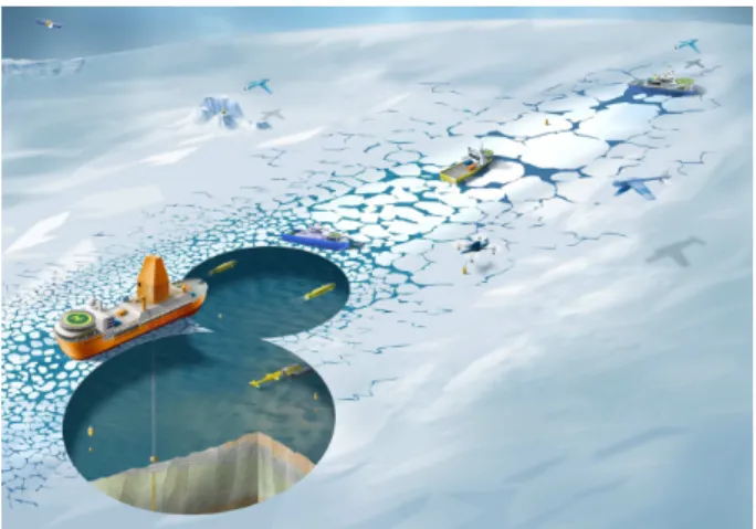
Close-field zone. The region of ice that most likely will reach the DP vessel. Detailed information about the ice feature geometry, ice thickness, ice concentration, ice drift velocity, and more may all be important for good DP performance (Metrikin et al.,2013). Up to a few hours upstream. The zones have different extents and no single sensor platform is able to perform all the monitoring tasks by itself. Eik and Løset (2009) motivates unmanned un-derwater vehicles (UUVs) as a tool in collecting ice in-telligence for ice defense, whereasHaugen et al.(2011) motivates unmanned aerial vehicles (UAVs) to do the same together several other sensor platforms in a col-laborative effort, see Figure1.
Figure 1: Illustration of a possible future Arctic dy-namic positioning operation that consists of many important components, including icebreakers, unmanned underwater vehicles, and unmanned aerial vehicles. Picture cour-tesy of Bjarne Stenberg.
The sensor platforms constitute an ice observation system, which is an integral part of both the ice defense and the dynamic positioning. Since the resources are constrained with respect to cost, physical, and practi-cal considerations, some kind of high-level task alloca-tion procedures need to choose the appropriate sensor platforms for the required monitoring tasks. This task allocation happens both before and during the opera-tion execuopera-tion:
In the planning phase, decisions such as the choice of immobile sensors, type and number of mobile sen-sor platforms are made. These choices are made based on the required level of information and re-dundancy for the particular operation in question.
fleet of singular or teams of mobile sensor net-works.
The dynamic planning allows for low response times in deployment and may facilitate real-time acquisition of information, so that important operational decisions can be made. There is a wide range of monitoring missions that may be needed in ice defensing. With respect to the mid-field and far-field zones, possible missions for remotely piloted aircraft systems (RPASs) are:
Mission 1. Iceberg and ice ridge detection, identifica-tion, and tracking.
Mission 2. Sea ice identification and dynamic cover-age.
2.1 Remotely Piloted Aircraft Systems in
Cold Regions
A remotely piloted aircraft system (RPAS) is a sub-group of the more general category of unmanned air-craft systems (UASs). The RPAS consists of all the components needed to operate such a system: one or several UAVs, a ground station including the pilot station, launch and recovery systems, communication equipment, and more (CAA–Norway,2014). An RPAS may be autonomous in the sense that the system can make its own decisions during the course of operation execution, but with the restriction that an operator can intervene and remotely pilot the UAVs.
The inclusion of RPASs in cold regions comes with a whole range of challenges that need to be addressed. Common keywords when talking about operations in Arctic regions are remoteness, darkness, and low tem-peratures. Robustness against these attributes is very important and may include sophisticated launch and recovery systems from ships (Crowe et al., 2012), ro-bust communication systems (Frew and Brown,2009), and fault-tolerant guidance, navigation, and control (GNC) systems. Other aspects that need to be ad-dressed include (Haugen et al., 2011; Crowe et al.,
2012): icing problems, vibration issues, water intru-sion, and airspace access. Norwegian research commu-nities working with problems connected to RPAS in cold regions includeAMOS(2014);Norut(2014); Sim-icon(2011).
Apart from GNC, one aspect of an autonomous air-craft system is its ability to create paths that help in solving some monitoring task. In a cold regions op-eration setting, one can think of many different tasks that need a specialized system that can perceive its en-vironment and make intelligent decisions based on the observations. In this manuscript, we briefly discuss the following ice observation sub-tasks: target tracking,
re-lated to Mission 1, and dynamic coverage control, re-lated to Mission2. We provide an overview of common components that have been used to solve the mentioned sub-tasks inHaugen and Imsland(2014b) andHaugen and Imsland(2014a), respectively. We will finally dis-play results from a hybrid field experiment of thetarget tracking task, which was first reported inHaugen and Imsland(2013b).
2.1.1 Target Tracking
Suppose a set of possibly hazardous icebergs and ice ridges has been detected in the far-field zone with the use of satellites. The acquired satellite data are of too coarse resolution to provide conclusive answers (Eik,
2008;Haugen et al.,2011). To confirm/refute the pos-sible hazards, current practices involve manned aircraft (Eik,2008) and reconnaissance vessels (Sheykin,2010). We motivate the use of UAVs as a tool which may re-duce costs and environmental footprint when solving this monitoring task. The task is formulated as atarget tracking objective and approached by assuming that a small number of UAVs is dispatched to remotely gather more information before further actions are taken.
The target tracking problem is the task of monitor-ing mobile or immobile objects usmonitor-ing (usually mobile) sensor agents. Many problems can be cast as a tar-get tracking problem, so the literature is rich on vari-ous approaches, seeHaugen and Imsland (2014b) and references therein. Haugen and Imsland(2014b) clas-sify contributions in literature as “nmtono” tracking, wherenmis the number of sensors andnois the number of objects. The above defined problem is a multi-target tracking objective, where the number of mobile sensor agents are possibly more than one.
In solving the target tracking problem, contributions usually choose between two main methodologies: re-source allocation and information-driven approaches. In the resource allocation problem, the targets are pre-scribed to be visited a predefined number of times. It is formulated as a modified traveling salesperson problem (Rathinam et al., 2007; Looker, 2008; Savla et al., 2008), often taking the limited turning radius of the mobile sensor into account. Unlike resource al-location, information-driven methods define the visi-tations of the targets according to some information reward. Information gradients are usually utilized in the formulation of optimization problems, which are seeking to minimize measures related to the informa-tion level, either minimize time between target mea-surements (Tang and ¨Ozg¨uner, 2005), maximize ob-servation time (Parker, 1999), or minimizing the tar-gets’ estimation error covariance (Haugen and Imsland,
2.1.2 Dynamic Coverage Control
Imagine you want to get an awareness map of a bounded region in the mid-field zone. When creat-ing this awareness map, one task may be to get more detailed information about relevant ice conditions, for instance the ice concentration, which is the area frac-tion of ice versus open water. Current approaches in-clude using satellites, reconnaissance vessels, and ma-rine radars (Sheykin,2010). We propose to use UAVs to cover the region of interest. Since the ice has a drift-ing velocity, the task can be formulated as adynamic coverage problem.
Wang and Hussein(2012) describes the dynamic cov-erage problem as the problem of covering a given region using mobile sensor networks. The desired information to be gathered changes in both time and space, so a non-dynamic coverage algorithm may not be sufficient to capture the information with the required level of accuracy. The monitoring task is therefore to perform state estimation of some distributed parameter system (DPS), usually described as a partial differential equa-tion (PDE).
Previous work on state estimation dynamic cover-age falls under two main approaches: optimal con-trol formulations (Burns et al., 2009; Choi and How,
2010;Haugen and Imsland,2014a), and gradient-based guidance algorithms (Demetriou and Hussein, 2009;
Demetriou, 2010; Haugen et al., 2012). In the opti-mal control problem (OCP) formulation, one seeks to minimize some kind of objective functions that quan-tify the information reward of visiting a particular re-gion. The formulations often use a measure based on the estimation error covariance dynamics (Burns et al., 2009; Choi and How, 2010), but to facilitate computational speed, simplified information dynamics has also been proposed (Haugen and Imsland, 2014a). Gradient-based guidance algorithms are more compu-tationally efficient, but often rely on locally available estimation error to guide the vehicles (Demetriou and Hussein, 2009; Demetriou,2010;Haugen et al.,2012).
2.2 Optimization-Based Path Planning
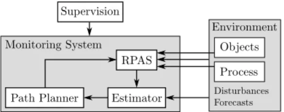
We approach the two tasks identified as target track-ing and dynamic coverage control by considertrack-ing two separate monitoring systems. Both systems have three common components:
RPAS: Remotely piloted aircraft system that acts as a mobile sensor network. The mobile sensors pro-vide measurements of the environment. Depend-ing on the which task is beDepend-ing solved, they provide measurements of objects or a distributed process.
Estimator: Prepares collected measurements and other inputs to return the most likely model state
and parameters of the mobile sensors and the ob-served environment.
Path Planner: Generates guidance inputs of when and where we want the mobile sensor to obtain mea-surements of the environment.
Figure 2 displays an overview of the system compo-nents. The Supervision component has the role as a dynamic mission planner. It is responsible for deciding how many mobile sensors to deploy, which region or objects to cover, and other high-level decisions.
Figure 2: Key components of the monitoring systems used to solve the target tracking and dynamic coverage control problems.
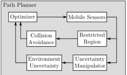
ThePath Planner component solves a dynamic opti-mization problem motivated by the information-driven approach. It contains mathematical descriptions of various modules that are needed to create meaning-ful guidance inputs (cf. Figure3). The mobile sensor agents are described using simple ordinary differential equations (ODEs) with maneuverability constraints. The mobile sensors need to satisfy collision avoidance requirements and stay within permitted regions of op-eration. The objective of the path planner is to manip-ulate the commanded input of the mobile sensors such that some reward function is maximized. The reward function depends on a description of the monitored en-vironment’s uncertainty. The environment uncertainty can be controlled using the mobile sensor agents, which act as uncertainty manipulators. For instance, in the case of target tracking, the environment uncertainty can be described as the sum of all the object’s state es-timation error covariances. The uncertainty can then be manipulated by the moving agent’s sensing capabil-ity, which reduces the uncertainty close to the agent’s location.
Figure 3: Conceptual modules in the path planner.
3 Path Planning for Target
Tracking
Suppose that there are some objects moving with al-most constant velocity that we want to keep track of. We assume that we have estimated initial positions of the objects at timet0, but that the objects’ states are uncertain. An unmanned aerial vehicle is able to sense the objects using for instance a camera with a lim-ited field of view (FOV). Since the FOV is limlim-ited, the objects cannot necessarily be observed simultaneously. The objective is thus to steer the mobile sensor such that all the objects’ states can be estimated.
Let{ned}denote a right-handed stationary reference frame whose axes denote north, east, and down coordi-nates, respectively. Define for each object inIn
o =:O
the state vectorχo:= col(No, Eo), which are north and east coordinates. Let the initial position of objectobe
χo(t0) =χo,0, (1a)
and the corresponding dynamics ˙
No(t) =vN,o+wN,o(t), (1b) ˙
Eo(t) =vE,o+wE,o(t), (1c) where po := col(vN,o, vE,o) is the known velocity pa-rameter vector, and col(wN,o(t), wE,o(t)) =: wχ
o(t) ∼
(0, Qo(t)) is process noise.
The states of the objects are random variables and are equipped with uncertainty measures. More specif-ically, ∀o ∈Owe define E(χo(t)) = ˆχo(t) as the state estimate ofχo(t). For eacho∈O, we define the state estimation errors as
˜
χo(t) =χo(t)−χoˆ (t), (2a) which gives the estimation error covariance
Po(t) = cov( ˜χo(t),χo˜ (t)). (2b) This matrix quantifies the uncertainty of objecto.
To accommodate feasible trajectories for the mo-bile sensor, we consider a low-fidelity constant-altitude
kinematic vehicle model with the bank angleuθ(t) as control input. Let xN(t) and xE(t) denote the north and east position of the sensor, and ψ(t) ∈ S the right-hand screw z-axis rotation of a body-fixed ref-erence frame {b} relative to {ned}. Define x(t) := col(xN(t), xE(t), ψ(t)) with the initial condition
x(t0) =x0. (3a)
The dynamics is ˙
xN(t) =Vacos(ψ(t)), (3b) ˙
xE(t) =Vasin(ψ(t)), (3c) ˙
ψ(t) = g
Vatan(uθ(t)), (3d)
where the constant parameters Va and g are the pos-itive airspeed and the standard gravity, respectively. We constrain the commanded bank angle so that the resulting state trajectories are sufficiently conservative and feasible. For allt∈R≥0 anduθ,L, uθ,H ∈Slet
uθ,L≤uθ(t)≤uθ,H. (3e) We also restrict the planar position of the mobile sen-sor. In particular, we define a closed convex polygon
K :={y ∈ R2 :Ay ≤b}, where A and b have appro-priate dimensions, so that x(t) is constrained for all
t∈R≥0by
x(t)∈ K ×S=:X. (3f)
Problem 1. Perform state estimation of the objects
o ∈In
o of (1) for all t ∈[t0, T], where T is the final
time of interest. This should be accomplished by deter-mining a feasible input uθ(t)for the mobile sensor (3) to obtain measurement intervals of all the objects.
We need to develop differential equations based on (2b) where the benefit of the mobile sensor is incorpo-rated. The objective is to minimize the uncertainties of the objects’ states to allow probable estimates of the objects future state trajectories. The task includes gen-erating feasible trajectories for the mobile sensor. The problem will be approached by formulating and effi-ciently solving a receding horizon optimization prob-lem that mathematically describes the objective. A sub-task is to find a plausible parametrization of the mobile sensor’s influence on the objects’ covariance dy-namics.
3.1 Measurement Models
Write the two-dimensional Cartesian coordinates of the mobile sensor as ̺(t) := col(xN(t), xE(t)). Further,
the objects simultaneously. We use sampling functions (Tricaud and Chen, 2012) that depend on the coordi-nates of the mobile sensor to reflect how the output vector is sampled by the sensor. In this context, the output vector is a vector function that depends on the planar position of an object being monitored.
Define the family of scalar sampling functions asW and let B be the codomain of this family. Let w : R≥0×R2×R2×S→Band define a diagonal matrix function W(t, ̺(t), q(t), ψ(t)) = w(t, ̺(t), q(t), ψ(t))× I2 with codomain ∈ B2×2. The shaped measurement vector is therefore defined as
yw(t) =W(t, ̺(t), q(t), ψ(t))y(t). (4) In our particular application we assume that the mobile sensor is capable of measuring an object’s position, so the noise-free output function is for eacho∈O
yo(t) =Coqo(t), (5) whereCo=I2. The role of the sampling function is to shapethe output function connected to an object. The output is switched off (set to zero) whenever the object is outside the measurement reach of the mobile sensor. A shaped measurement vector therefore captures the case where a measuring device has a limited field of view, for instance an image obtained from an optical device.
3.1.1 Non-Smooth Sampling Function
The purpose of this model is to simulate that the mea-suring device has a field of view in which it is able to obtain measurements. This includes for instance the cases of roll and pitch stabilized downward-looking op-tical devices and spectrometers.
Let ∆zi > 0, i ∈ {1,2} and define ∆z :=
col(∆z1,∆z2), withz= col(z1, z2). We define the
two-dimensional FOV metric as a weighted infinity norm
kxkFOV,∆z := max
|z 1| ∆z1
, |z2|
∆z2
. (6)
Suppose the position ̺(t) of a sensor is the ori-gin of a body-fixed Cartesian coordinate system {b}
. Further suppose the orientation ψ(t) of {b}
is defined relative some stationary reference frame
{i} following the right-hand rule. Let BC−1 :=
{0,1} be the codomain of a binary sampling func-tion wC−1 :R≥0×R2×R2×S→B
C−1 such that the
codomain is nonzero only if a coordinate point q(t)∈
R2 of an object is within the convex set formed by a FOV metric. The two-dimensional rotation matrix is
R(ψ) =
cosψ −sinψ
sinψ cosψ
. (7)
We can write the binary sampling function as
wC−1(t, ̺, q, ψ) :=
( 1,
RT(ψ)(q−̺) FOV,∆
z <1
0, otherwise.
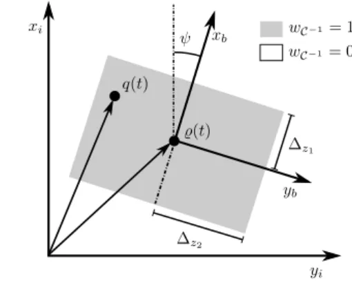
(8) Figure4 graphically illustrates the behavior of the bi-nary sampling function. We see that ∆z1 and ∆z2
quantify respectively the field of view inxb andyb di-rection of the body-fixed reference frame.
Figure 4: The non-smooth sampling function is one for
q(t) inside the box and zero otherwise. xiand
yidenote the axes of the stationary reference frame.
3.1.2 Smooth Sampling Function
In some cases, for instance in an optimization problem, a continuously defined sampling function with positive codomain may be preferred as an approximation to some non-smooth sampling function. LetBC∞ :={w∈
R : 0≤ w ≤1}. Define a smooth sampling function
wC∞(t, ̺, q, ψ) :R
≥0×R2×R2×S→BC∞, which is 1
if̺=qand less than 1 otherwise.
Example 1. LetKi∈In∈Π2, andq˜=q−̺. A possible
smooth sampling function is the linear combination of
ntwo-dimensional Gaussian functions, for instance
wC∞(t, ̺, q, ψ) :=
X
i∈In
λie−q˜TR(ψ)KiRT(ψ)˜q , (9)
where P
i∈Inλi = 1, λi ≥0. The purpose of having a
-5000 -2500 0
2500 5000 -5000
-2500 0 2500
5000 0
1
wC∞
˜
q1 [m]
˜
q2 [m]
wC∞
0.2 0.4 0.6 0.8 1
Figure 5: A smooth sampling function. The axes rep-resent col(˜q1,q˜2) = ˜q= (q−̺), which is the relative planar coordinate between an object and a sensor.
3.2 Path Planner
3.2.1 Adapted Covariance Dynamics
The estimation error covariance (2b) of the objects quantify the uncertainties of the state vector. We want to reduce these uncertainties by measuring the objects using the mobile sensor. The covariance response of the objects can be described by the corresponding equation in the continuous-time extended Kalman filter (Simon,
2006). We present in the following a version with both time-varying process noise and measurement matrices. To model the mobile sensor’s influence on the object covariance dynamics we make use of the measurement models presented in Section3.1. More specifically, we use the smooth sampling function to define a diagonal matrix function Wo for the sensor’s influence on each object. We get∀o∈O
Wo(t, ̺, qo, ψ) =wC∞,o(t, ̺, qo, ψ)×I2. (10)
The motivation for using smooth sampling functions is that the chosen solver needs smoothness and curvature to find a solution to the optimization problem. Hence, non-smooth sampling functions need to be approxi-mated using smooth sampling functions. The proposed shaping can be tuned in such way that the codomain approximates the behavior of a measuring device with a limited field of view such as a camera. The mobile sensor will significantly affect the covariance dynamics of the object if it is sufficiently close to it. The closer the mobile sensor is to the object, the bigger stabilizing impact it will have on the object’s covariance.
For each object o ∈ O let ˆχo(t) be the solution to the initial value problem (IVP) (1) withχo(t0) = ˆχo,0 which is the best estimate at time t0. Then, the pre-dicted trajectory for object o is ˆχo(t). We use the above matrix sampling functions to produce vehicle-dependent shaped versions of the measurement opera-torsCo of the objects along the predicted trajectories
ˆ
χo(t) = ˆqo(t). The measurement operators of the ob-jects are the identity matrices, so by using (10), we simply get for each objecto∈O
Cw
o(t) =wC∞,o(t, ̺,qo, ψˆ )×I2. (11)
When the mobile sensor is sufficiently far away from the object, the shaping of the measurement should be so little that it in practice does not affect the covariance: the mobile sensor is not able to measure the object. For the sensor to still be attracted to distant objects, we propose to manipulate the process noise matrices
Qo(t). We use a non-vanishing sampling function to reduce the process noise when a sensor is close to an object. In this way, the mobile sensor’s movement will always affect the covariance of the objects, but only slightly. Define for all objectso∈O
Qw
o(t, ̺,qo, ψˆ ) =Qo(t) (1−wC∞(̺,qo, ψˆ )). (12)
We use the vehicle-dependent time-varying expres-sions defined above to define the covariance dynamics of each objecto∈O. The differential Riccati equation of objectois
˙
Po(t) =Qw o −PoC
wT
o R−
1
o C w
oPo, (13a)
Po(t0) =Po,0, (13b)
where we have omitted the arguments of the expres-sions and used that the Jacobian of the object dynam-ics (1) is the zero matrix.
3.2.2 Dynamic Optimization Problem
The object monitoring can be formulated as a Bolza-type OCP. Let t0, tf ∈ R≥0 respectively denote the start and the end of the optimization horizon. The decision variable is the control inputuθ(t). LetP(t) := bdiago∈O(Po(t)).
We define the Lagrange term as ΦL(t, uθ) =
Z tf
t0
tr(P(t) diag(vL(t)))
+duθ
dt
T
Γ(t)duθ
dt +u
T
θΞ(t)uθdt, (14a)
where for eacho ∈ Owe have vL(t) := col
o∈O(vLo(t))
with vL
o(t) ∈ R2≥0 and the scalar functions Ξ(t) > 0,Γm(t) > 0, which all are time-varying design
vari-ables. Notice that in the presented applicationuθ is a scalar. The Mayer term is
ΦM(tf) = tr(P(tf) diag(vM)), (14b)
wherevM := col
o∈O(vMo )∈R2 no
the objects’ covariance dynamics, that is, ∀t∈[t0, tf],
∀o∈O:
min
uθ
ΦL(t, uθ) + ΦM(tf) (15a)
s.t. (3),(13). (15b) The solution to (15) provides us with the input vector
u⋆
θ(t)∈Uin the intervalt∈[t0, tf]. Given the variables u⋆
θ, ˆx0, we can solve the IVP formed by (3) over the
optimization horizon. This results in an optimal mobile sensor state trajectory, denoted as
x⋆(t)∈X, t∈[t0, tf]. (16) Equation (16) serves as guidance input to the aircraft.
3.2.3 Receding Horizon
Suppose we want to monitor the objects in the time intervalT:= [t0, T]. IfT is sufficiently large, the opti-mization problem (15) becomes very difficult to solve in real time. To overcome computation time issues, we solve the optimization problem in a receding horizon fashion. This involves successively solving optimiza-tion problems with shorter time horizons. There are several factors that motivate this design decision:
(i) Too long time horizons may make the optimiza-tion problem computaoptimiza-tionally intractable due to the problem size.
(ii) There are modeling inaccuracies, so the predicted object trajectories may drift away from the true trajectories.
(iii) Some conditions change, for instance a new object should be monitored.
By solving the optimization problem with receding horizons, the formulation can take into consideration updated information to improve the monitoring perfor-mance. Each time horizon overlaps with neighboring horizons. We utilize only a sub-interval of an optimized control input interval. Let kt ∈ N1 be the number of optimization intervals and Tk := [t0,k, tf,k] be the op-timization horizon for thekth iteration. For horizonk
we have t0,k < te,k < tf,k, where te,k is the final time
for which we use thekth iteration’s control input. The switch to the next iteration’s control input is therefore equal to the utilization time of the preceding iteration:
t0,k+1≡te,k.
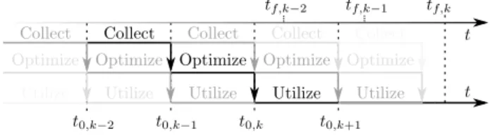
Consider thekth iteration of the monitoring process (see Figure6). We divide it into a three-step procedure of collecting, optimizing, and utilizing. The first step, which is performed by theEstimator, involves collect-ing measurements of the objects’ and sensor’s states. At timet0,k−1the collected information so far is used to perform state and parameter estimation. This involves predicting the future state of the objects and sensor
at time t0,k. The next step is to optimize by solving
(15) to obtain the desired path (16). This step is ac-complished by thePath Planner. The optimized paths should be readily available by the timet0,k, since they
at this time instant should be utilized by the RPAS, which is the final step.
Figure 6: The monitoring system consists of a three-step procedure of collecting, optimizing, and utilizing.
The three steps of the procedure execute concur-rently with earlier and later time steps: when the moni-toring system is optimizing for iterationk, it is collect-ing for iteration k+ 1, and utilizing iteration k−1. Figure6 illustrates the three-step procedure.
4 Case Study
4.1 Implementation
To efficiently solve the OCP (15), we choose a direct transcription approach where both the state and con-trol variables are discretized into a finite-dimensional nonlinear programming (NLP) problem. The simulta-neous collocation of finite elements is used to obtain Lagrange interpolation polynomial descriptions of the state variables. The control input is piecewise con-stant, whereas the states are described using K-point Radau collocation, for details consultBiegler(2010).
The resulting large-scale NLP formulation benefits from being sparse and having structure. These prop-erties can be exploited using an efficient NLP solver. We formulate the problem in the symbolic framework CasADi (Andersson et al., 2012), which provides the necessary derivative information required by both the extended Kalman filter and the NLP solver. The CasADi library contains an interface for the primal-dual interior-point NLP solver IPOPT (W¨achter and Biegler, 2006). IPOPT is compiled with OpenBLAS (Xianyi et al., 2012) and the linear algebra sparse di-rect solver MA27 (HSL,2011).
An initial desired sensor path is provided a priori be-cause it needs to be available when the first optimiza-tion is running. Once an OCP has finished, solving the mobile sensor dynamics with the provided initial condi-tion and control inputs, results in a new optimal path. The performance of the discretized optimization prob-lem benefits from good initial conditions. We initialize the object state and covariance variables by solving the matching IVPs with expected closed-loop behavior of the mobile sensor given its respective predicted initial condition. Since a new optimization horizon goes be-yond the previous, we use the previous iterations final control input as extrapolation.
4.2 Experiment Setup
We are going to solve Problem1, which was presented in Section 3 with no = 3. We numerically simulate the objects under surveillance and use an UAV as the mobile sensor. We assume that the UAV is capable of observing the objects with a pitch and roll stabi-lized downward-looking optical camera. Since no real objects are going to be observed, we simulate this be-havior by providing object measurements at a sam-pling frequency of 1 Hz whenever the simulated object is within the field of view of ∆z1 = ∆z2 = 300 m using
(8).
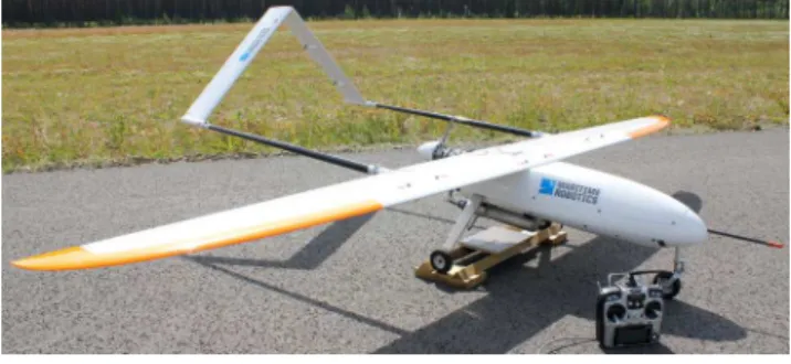
The RPAS is provided byMaritime Robotics(2013). It consists of a Penguin UAV B (Figure 7) fromUAV Factory(2013) with a Piccolo autopilot and the flight management software Piccolo Command Center from
Cloud Cap Technology (2013). This system is used with waypoint-tracking capability, so the continuous state trajectories provided by the path planner are sampled at a frequency of 1/8 Hz. The sampled north and east coordinates are combined with a constant al-titude of 600 m and transformed into laal-titude and lon-gitude decimal degrees (WGS84). This information is written to compatible waypoint files and manually up-loaded to the aircraft autopilot by a flight operator in a timely manner. The path-planning algorithm itself is run on a laptop computer and receives aircraft teleme-try data at 1 Hz from the Piccolo Command Center trough a TCP/IP connection. From the telemetry data the GPS coordinates and orientation are utilized by the path planner.
The experiment was executed at Eggemoen Avia-tion and Technology Park, Ringerike, Norway. An ex-tended visual line-of-sight (EVLOS) airspace was al-located, with additional field observers on a lookout for unscheduled air traffic. A nominal circular path within the confined airspace is uploaded a priori to make it easier to initialize the path planning algo-rithm. Once started, the path-planning framework received a mobile sensor initial condition of ˆx(t0) =
Figure 7: Maritime Robotics’ Penguin B from UAV Factory that was used during the experiments.
col(1621.63,−640.87,6.00) at t0 = 0.74 s. The bank angle is constrained to be within [uθ,L, uθ,H] = [−π
9 ,
π
9]. This is more conservative than what the autopilot actu-ally can manage, but software-in-the-loop simulations suggest better path-following performance under this constraint. The standard gravityg is set to 9.81 m s−2 and the airspeedVa is 28 m s−1.
The initial conditions of the objects are ˆχ1(t0) = col(1360,700), ˆχ2(t0) = col(2946,−539), and ˆχ3(t0) = col(2400,440), wheret0= 1.00 s. The velocity parame-ters arep1 = col(−1.15,−0.96),p2 = col(−0.82,0.57), and p3 = col(0,0). The estimation error covariance matrices are Po∈I3(t0) = I2. The process noise
spec-tral densities areQo∈I3= 0.1I2and measurement noise
spectral densities areRo∈I3 = 10I2.
The smooth weighting functions for the measure-ment matrices areWo∈I3 =wC∞(·)I2, using the
weight-ing function of Example 1 with n = 1, K1 = 3.3× 10⁻⁵I2. The weighting function of (12) is the same for all objects, also defined as in Example 1 with n = 1 andK1= 5.2×10⁻⁷I2.
The optimization horizon is 120 s and the sampling interval 60 s. A 2-point Radau collocation is used for discretization of the state variables with a total for 40 finite elements at each optimization horizon. The con-trol input is piecewise constant with 20 finite elements over the horizon. Meters are scaled by 1/100 in the op-timization problem and the following variables are used in the scaled OCP: vL
o∈I3(t) = 25 col(1,1), Γ(t) = 5,
Ξ(t) = 0, andvM
o∈I3= 40 col(1,1).
4.3 Results
waypoint files, so it was stressful for the flight operator to execute this task. At several occasions the operator failed to switch to the new waypoint file in due time, resulting in the autopilot to perform a re-run of the currently tracked waypoint. This basically means that the aircraft did not fly sufficiently close to the waypoint and it was not properly visited. This behavior does not coincide well with the path planner, so the experiment had to be reset. The results in the following capture a run where this problem did not occur. Another run is illustrated inHaugen and Imsland(2014b).
0 15 30 45 60
1 2 3 4 5 6
Solv
e
time
[
s
]
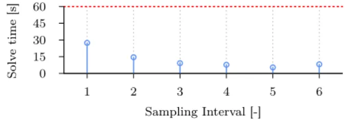
Sampling Interval [-]
Figure 8: The computation time of each optimization problem is always less than 30 s. This gives the operator enough time to upload the new waypoints within the sampling period of 60 s. As can be seen in Figure 9, the planned paths were within the constraints of the vehicle model. Neverthe-less, no wind speeds were included in the path plan-ning, so the aircraft still had to struggle to properly follow the planned path. The autopilot is set with a constant airspeed. With nonzero wind velocity, the aircraft did move along the path, but the temporal ex-ecution was incorrect. As a result, the aircraft might come too late or too early to a specific location. This was not a huge problem in our case, but by including estimates of the wind velocity in the vehicle model of the path planner and/or allowing some leeway in the desired airspeed, this error can perhaps be reduced. We did try the former approach with an extended Kalman filter, but likely due to poor wind velocity estimates, we did not succeed to obtain satisfactory results.
A plot showing the experiment with north and east coordinates are displayed in Figure 10. The shaded polygon is the admissible operation region. Dashed lines represent optimized/predicted trajectories, and solid lines are filtered values. An object marker indi-cates that the object has been observed by the aircraft (there are also markers att0). An aircraft marker indi-cates the instant of switching from one sampling inter-val to the next, which occurs every 60 s. We see that the aircraft is able to follow the planned paths fairly well and does observe the objects under surveillance without violating the admissible region.
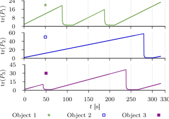
The uncertainty of an object’s position is signifi-cantly reduced every time it is being observed. Once
-0.4 -0.2 0 0.2 0.4
330
0 50 100 150 200 250 300
uθ
[
ra
d
]
t[s]
Figure 9: The optimized control input that are used together with the low-fidelity vehicle model to construct the desired paths for the mobile sensor. The input remains within the upper and lower constraint, which are indicated by dashed lines.
an object leaves the FOV of the mobile sensor, the uncertainty increases. Figure11illustrates this behav-ior during the experiment. It should be pointed out that the objects were simulated without noise, so the path planner perfectly predicted their future locations. Even if noise had been included in the object simula-tions, the mobile sensor still might have been able to find the objects, since they were observed fairly often, and that the FOV was relatively large. In the opposite case, an unobserved object leads to greater uncertainty and higher priority at the next optimization horizon. This does not remedy the fact that an object was not where it was predicted to be, and the object might still remain unobserved. The current framework does not handle the event of missed observations, and this should be considered as a relevant extension. More-over, if an object leaves the region of interest, or if a new one arrives, this can easily be added to the path planner at the next sampling interval.
5 Concluding Remarks
The optimization-based path planner for object surveillance devised in Haugen and Imsland (2013b) has been successfully demonstrated in a full-scale ex-periment. Although the planned paths can be followed successfully, including wind velocity estimates in the vehicle model of the path planner, or manipulating the desired airspeed of the autopilot is advised to improve path-tracking performance.
monitor--1000
-500
0
500
1000
-500 0 500 1000 1500 2000 2500 3000
East
[
m
]
North [m]
Sensor 1 Object 1
Object 2 Object 3
Figure 10: The mobile sensor performs remote sensing of the three objects in question. The dashed line represents optimized/predicted trajec-tories, whereas solid lines are filtered val-ues. Every aircraft marker represents the instant when a new sampling interval is uti-lized. An object observation is represented with a line marker. The shaded polygon is the admissible region.
0 8 16 24
tr
(
P1
)
0 20 40 60
tr
(
P2
)
0 15 30 45
330
0 50 100 150 200 250 300
tr
(
P3
)
t[s]
Object 1 Object 2 Object 3
Figure 11: The trace of each object’s covariance ma-trix. An object observation is indicated by a significant reduction in the trace magnitude.
ing task, where an instance of the monitoring systems presented herein executes within each partition. The independent instances are connected to a higher-level Supervisioncomponent, which is responsible for ensur-ing that sub-tasks are properly delegated.
Other further work include extending the framework to handle missed observations, allowing simultaneous detection and tracking, and executing a more real-life experiment with real objects. It would also be inter-esting to see an execution without human-in-the-loop, both allowing more objects to be observed and display-ing truly autonomous surveillance.
Acknowledgments
Research partly funded by Research Council of Norway (RCN) KMB project no. 199567: “Arctic DP”, with partners Kongsberg Maritime, Statoil, and DNV GL, and partly by RCN project no. 223254: CoE AMOS. The authors would like to thank Carl Erik Stephansen, Vegard Hovstein, and other involved parties at Mar-itime Robotics for their professional and flawless exe-cution of the practical sides of the experiments. The authors also appreciate the assistance provided by Lars Semb, Anders Willersrud, and Anne Mai Ersdal during the field experiment period. Additionally, the authors would like to thank Francesco Scibilia and Esten Ingar Grøtli for constructive feedback on the manuscript.
References
AMOS. Center for Autonomous Marine Op-erations and Systems. 2014. URL http: //www.ntnu.edu/amos/centre-for-autonomous-marine-operations-and-systems.
Andersson, J., ˚Akesson, J., and Diehl, M. CasADi: A symbolic package for automatic differentiation and optimal control. In S. Forth, P. Hovland, E. Phipps, J. Utke, and A. Walther, editors, Recent Advances in Algorithmic Differentiation, volume 87 ofLecture Notes in Computational Sci. and Eng., pages 297– 307. Springer-Verlag, Berlin Heidelberg, Germany, 2012. doi:10.1007/978-3-642-30023-3 27.
Arctic Marine Solutions. 2014. URL www. arcticmarinesolutions.se.
Biegler, L. T. Nonlinear Programming: Con-cepts, Algorithms & Applications to Chemical Processes. SIAM, Philadelphia, PA, 2010. doi:10.1137/1.9780898719383.
fil-tering and smoothing with mobile sensor networks. In Proc. 17th Mediterranean Conf. Control & Au-tomation, MED ’09. Thessaloniki, Greece, pages 181–186, 2009. doi:10.1109/MED.2009.5164536. CAA–Norway. Civil Aviation Authority – Norway,
RPAS-FAQ. 2014. URLwww.luftfartstilsynet. no/selvbetjening/allmennfly/RPAS-FAQ/. Choi, H. and How, J. P. Continuous trajectory
planning of mobile sensors for informative fore-casting. Automatica, 2010. 46(8):1266–1275. doi:10.1016/j.automatica.2010.05.004.
Cloud Cap Technology. 2013. URL http://www. cloudcaptech.com.
Crowe, W., Davis, K. D., la Cour-Harbo, A., Vihma, T., Lesenkov, S., Eppi, R., Weatherhead, E. C., Liu, P., Raustein, M., Abrahamsson, M., Johansen, K.-S., and Marshall, D. Enabling science use of unmanned aircraft systems for arctic environmen-tal monitoring. Technical Report 6, Arctic Moni-toring and Assessment Programme (AMAP), Oslo, Norway, 2012. URL http://amap.no/documents/ download/938.
Demetriou, M. A. Guidance of mobile actuator-plus-sensor networks for improved control and es-timation of distributed parameter systems. IEEE Trans. Autom. Control, 2010. 55(7):1570–1584. doi:10.1109/TAC.2010.2042229.
Demetriou, M. A. and Hussein, I. I. Estimation of spatially distributed processes using mobile spatially distributed sensor network. SIAM J. Control Op-tim., 2009. 48(1):266–291. doi:10.1137/060677884. Edmond, C., Liferov, P., and Metge, M. Ice and iceberg
management plans for shtokman field. InProc. OTC Arctic Technol. Conf. 2011. Houston, TX, pages 1–9, 2011. doi:10.4043/22103-MS.
Eik, K. Review of experiences within ice and ice-berg management. J. Navig., 2008. 61(4):557–572. doi:10.1017/S0373463308004839.
Eik, K. and Løset, S. Specification for a sub-surface ice intelligence system. In Proc. ASME 28th Int. Conf. Ocean, Offshore and Arctic Eng., OMAE2009. Honolulu, HI, pages 103–109, 2009. doi:10.1115/OMAE2009-79606.
Fossen, T. I. Handbook of Marine Craft Hydrodynam-ics and Motion Control. John Wiley & Sons Inc., Hoboken, NJ, 2011. doi:10.1002/9781119994138.
Frew, E. W. and Brown, T. X. Networking issues for small unmanned aircraft systems. J. Intell. Robot. Syst., 2009. 54(1–3):21–37. doi: 10.1007/s10846-008-9253-2.
G¨urtner, A., Baardson, B. H. H., Kaasa, G.-O., and Lundin, E. Aspects of importance related to arctic dp operations. In Proc. ASME 31th Int. Conf. Ocean, Offshore and Arctic Eng., OMAE2012. Rio de Janeiro, Brazil, pages 617–623, 2012. doi:10.1115/OMAE2012-84226.
Hamilton, J., Holub, C., Blunt, J., Mitchell, D., and Kokkinis, T. Ice management for support of arc-tic floating operations. InProc. OTC Arctic Tech-nol. Conf. 2011. Houston, TX, pages 1–12, 2011. doi:10.4043/22105-MS.
Haugen, J., Grøtli, E. I., and Imsland, L. State estimation of ice thickness distribution using mo-bile sensors. In Proc. IEEE Multi-Conf. Syst. Control. Dubrovnik, Croatia, pages 336–343, 2012. doi:10.1109/CCA.2012.6402649.
Haugen, J. and Imsland, L. Optimization-based au-tonomous remote sensing of surface objects using an unmanned aerial vehicle. In Proc. European Con-trol Conf. (ECC). Zurich, Switzerland, pages 1242– 1249, 2013a. URLhttp://ieeexplore.ieee.org/ stamp/stamp.jsp?tp=&arnumber=6669610.
Haugen, J. and Imsland, L. UAV Path Planning for Multitarget Tracking with Experiments. In Proc. 2nd IFAC Workshop Res., Develop. and Educ. Un-manned Aerial Syst.Compi`egne, France, pages 316– 323, 2013b. doi:10.3182/20131120-3-FR-4045.00061. Haugen, J. and Imsland, L. Monitoring an advection-diffusion process using aerial mobile sensors. Un-manned Systems, 2014a. Submitted.
Haugen, J. and Imsland, L. Monitoring moving objects using aerial mobile sensors. IEEE Trans. Control Syst. Technol., 2014b. Accepted.
Haugen, J., Imsland, L., Løset, S., and Skjetne, R. Ice observer system for ice management operations. In Proc. 21st Int. Offshore and Polar Eng. Conf.Maui, HI, pages 1120–1127, 2011.
HSL. A collection of Fortran codes for large scale sci-entific computation. 2011. URL http://www.hsl. rl.ac.uk.
Keinonen, A. J. Ice management for ice offshore op-erations. InProc. OTC Arctic Technol. Conf. 2008. Houston, TX, pages 1–15, 2008. doi: 10.4043/19275-MS.
Looker, J. R. Minimum paths to interception of a mov-ing target when constrained by turnmov-ing radius. nical Report DSTO-TR-2227, Defence Sci. & Tech-nol. Organisation, Canberra, Australia, 2008. URL
http://dspace.dsto.defence.gov.au/dspace/ bitstream/1947/9741/1/DSTO-TR-2227PR.pdf. Maritime Robotics. 2013. URL http://www.
maritimerobotics.com.
Metrikin, I., Løset, S., Jenssen, N. A., and Kerkeni, S. Numerical simulation of dynamic positioning in ice. Marine Technol. Soc. J., 2013. 47(2):14–30. doi:10.4031/MTSJ.47.2.2.
Moran, K., Backman, J., and Farrell, J. W. Deep-water drilling in the arctic ocean’s permanent sea ice. In J. Backman, K. Moran, D. B. McInroy, L. A. Mayer, and the Expedition 302 Scientists, editors, Proc. IODP, 302. Integraded Ocean Drilling Pro-gram Management Int., Inc., Edinburgh, UK, pages 1–13, 2006. doi:10.2204/iodp.proc.302.106.2006. Morbidi, F. and Mariottini, G. L. Active target
track-ing and cooperative localization for teams of aerial vehicles. IEEE Trans. Control Syst. Technol., 2013. 21(5):1694–1707. doi:10.1109/TCST.2012.2221092. Norut. Norut UAV remote sensing. 2014. URL
http://norut.no/en/satelitter-fjernmaling-og-ubemannede-fly.
Parker, L. E. Cooperative robotics for multi-target ob-servation.Intell. Autom. Soft Comput., 1999. 5(1):5– 19. doi:10.1080/10798587.1999.10750747.
Rathinam, S., Sengupta, R., and Darbha, S. A resource allocation algorithm for multivehicle
systems with nonholonomic constraints. IEEE Trans. Autom. Sci. Eng., 2007. 4(1):98–104. doi:10.1109/TASE.2006.872110.
Savla, K., Frazzoli, E., and Bullo, F. Traveling sales-person problems for the Dubins vehicle. IEEE Trans. Autom. Control, 2008. 53(6):1378–1391. doi:10.1109/TAC.2008.925814.
Sheykin, I. B. Icebreaker reconnaissance for ice mange-ment: offshore experience. InProc. 20th IAHR Int. Symp. Ice. Lahti, Finland, pages 525–536, 2010. Simicon. Simicon Arctic UAS. 2011. URL http://
simicon.no/.
Simon, D. Optimal State Estimation. John Wiley & Sons Inc., Hoboken, NJ, 2006.
Tang, Z. and Ozg¨¨ uner, U. Motion planning for multitarget surveillance with mobile sensor agents. IEEE Trans. Robot., 2005. 21(5):898–908. doi:10.1109/TRO.2005.847567.
Tricaud, C. and Chen, Y. Optimal Mobile Sensing and Actuation Policies in Cyber-physical Systems. Springer-Verlag, London, UK, 2012. doi:10.1007/978-1-4471-2262-3 1.
UAV Factory. 2013. URLhttp://www.uavfactory. com.
W¨achter, A. and Biegler, L. T. On the implementa-tion of an interior-point filter line-search algorithm for large-scale nonlinear programming. Math. Pro-gramming, 2006. 106:25–57. doi: 10.1007/s10107-004-0559-y.
Wang, Y. and Hussein, I. I. Search and Classifica-tion Using Multiple Autonomous Vehicles. Springer-Verlag, London, UK, 2012. doi: 10.1007/978-1-4471-2957-8 1.