Original Article
Development of a model selection method based on the reliability
of a soft sensor model
Takeshi Okada, Hiromasa Kaneko, and Kimito Funatsu*
Department of Chemical System Engineering,
The University of Tokyo, Hongo 7-3-1, Bunkyo-ku, Tokyo 113-8656, Japan.
Received 13 December 2011; Accepted 27 March 2012
Abstract
Soft sensors are widely used to realize highly efficient operation in chemical process because every important variable such as product quality is not measured online. By using soft sensors, such a difficult-to-measure variable y can be estimated by other process variables which are measured online. In order to estimate values of y without degradation of a soft sensor model, a time difference (TD) model was proposed previously. Though a TD model has high predictive ability, the model does not function well when process conditions have never been observed. To cope with this problem, a soft sensor model can be updated with newest data. But updating a model needs time and effort for plant operators. We therefore developed an online monitoring system to judge whether a TD model can predict values of y accurately or an updating model should be used for both reducing maintenance cost and improving predictive accuracy of soft sensors. The monitoring system is based on support vector machine or standard deviation of y-values estimated from various intervals of time difference. We confirmed that the proposed system has functioned successfully through the analysis of real industrial data of a distillation process.
Keyword: soft sensor, process control, model selection, time difference, moving window
1. Introduction
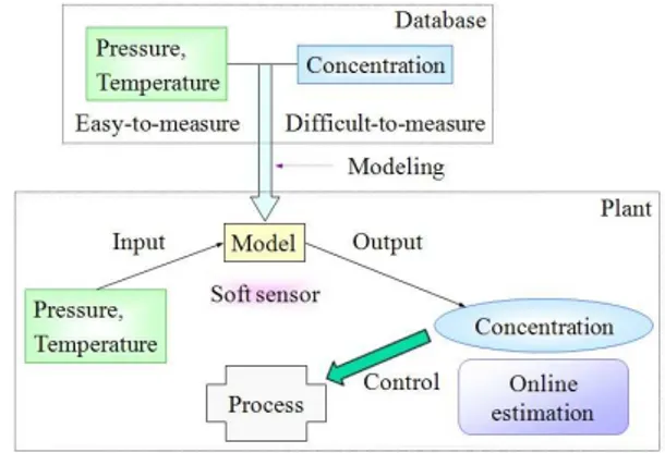
For realizing highly efficient operations, chemical processes must be controlled by using process variables such as pressure, temperature, concentration, flow, liquid level, and so on. However, every important variable such as product quality is not always measured easily because of technical difficulties, large measurement delays, high investment costs, and others. To estimate the difficult-to-measure variable y, soft sensors; (Kadlec et al., 2009) are widely used in chemical processes. By using soft sensors, y-values can be estimated with other process variables X, which are easily measured online. Figure 1 shows the basic concept of the soft sensors. By using the estimated values, the process can be controlled easily and promptly.
However, soft sensors have some practical difficulties. One of the crucial difficulties is that their predictive accuracy gradually decreases due to changes in the state of chemical plants, catalyzing performance loss, scale deposition, process
* Corresponding author.
Email address: [email protected]
http://www.sjst.psu.ac.th
drift, and others. In order to reduce the degradation of a soft sensor model, updating models were proposed (Kadlec et al., 2011). These models have high predictive ability because the models are adaptive to new operating conditions. However, the models are optimized for a certain period of operating time, and hence, need to be used carefully. Therefore, opera-tors have to check the model in terms of predictive accuracy of y for a long period of time and a relationship between X and y before practically applied. It takes significant time and efforts because there are many applications of soft sensors.
For solving these problems, Kaneko et al. (2011) developed a time difference (TD) model for reducing the efforts of updating models without the degradation of a soft sensor model. Though a TD model has a high predictive ability without updating the model, it does not function well when a process condition has never been observed. In order to cope with both the degradation and efforts for checking the models, we have attempted to develop a model selection method to achieve high predictive ability and reduce the efforts. This method is an online monitoring system to judge whether a TD model can predict values of y accurately or an updating model should be used for accurate prediction. By using the proposed method, we can reduce maintenance cost, which means time and efforts of detecting and eliminating abnormal data and checking the parameters of the model in model updating, and improve predictive accuracy of soft sensors.
2. Research Methodology
In this section, before describing a new model selec-tion method, we briefly explain tradiselec-tional multivariate statis-tical process control (MSPC) methods (Kourti, 2005). It is important to find variations in process variables because the prediction accuracy of a TD model is related to process con-ditions. Then, MSPC methods are applicable to estimate the prediction accuracy of a TD model. Many researchers developed data-based process monitoring methods to detect process variations (Bersimis et al., 2007; Kano et al., 2008). Two types of MSPC methods, the ensemble prediction method (EPM) (Kaneko et al., 2011) and support vector machine (SVM)-based MSPC methods (Kaneko et al., 2009) are used in this paper.
2.1 EPM
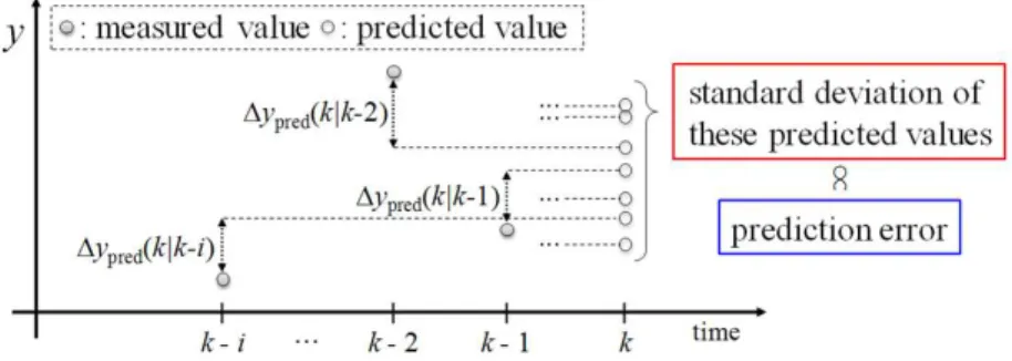
The EPM handles multiple y-values predicted by in-putting multiple intervals of time difference of X into a TD model. Figure 2 shows the basic concept of the EPM. To esti-mate a prediction accuracy of a TD model at time k, the TD model predicts multiple y-values from the multiple intervals of time difference of X, x(k|k-1), x(k|k-2), …, and x(k|k-i). Then, ypred values are predicted from each time, and ypred
values are calculated by using y(k-1), y(k-2), ..., and y(k-i) as follows:
( , 1) ( , 1) ( 1)
( , 2) ( , 2) ( 2)
( , ) ( , ) ( )
pred pred
pred pred
pred pred
y k k y k k y k y k k y k k y k
y k k i y k k i y k i
(1)
The EPM is calculated by standard deviation of these estimated y-values. When the EPM values are large, the process is changing and a TD model cannot predict accu-rately. When the EPM values are small, the process is static state and a TD model can predict accurately. The detail of EPM is written in Kaneko et al. (2011).
2.2 SVM-based MSPC Methods
Chemical processes are multivariable systems, and hence, it is important to consider a large number of mutually correlated variables. Therefore, MSPC has been developed to monitor such multivariable processes. The basic concept of MSPC is to determine the control limit of process variables, i.e. the normal condition of a process, and to detect data outside the control limit.
SVM is one of the nonlinear classification methods and it can determine the control limit. First, data measured in normal conditions are labeled as 1; data measured in ab-normal conditions are labeled as -1; and then, a discriminant model is constructed by using the SVM method with the labeled data. For improving the discriminant ability, principal component analysis (PCA) (Jolliffe, 1986) and independent component analysis (ICA) (Comon, 1994) are combined with the SVM in this study. By using PCA and ICA, we can extract
important components from process variables before con-structing SVM models. Figure 3 is the image of concon-structing SVM, PCA-SVM, and ICA-SVM. SVM relates X-variables and the label of data. In PCA-SVM and ICA-SVM, discrimi-nant models are constructed after extracting principal com-ponents and independent comcom-ponents from X-variables by using the PCA and ICA methods, respectively.
2.3 Proposed method
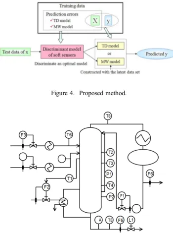
A TD model is mainly used, but when decreasing the prediction ability of a TD model, a moving window (MW) model (Qin, 1998) is used. A MW model is one of the updat-ing models and used for time series analysis and constructed with the latest data set of X and y. Figure 4 shows the basic concept of the proposed method.
For developing a model discriminating an optimal soft sensor, first, a TD model and a MW model are constructed by training data and prediction error are calculated by using the models. The discriminant model is constructed by using MSPC method between X and the variable that is labeled as 1 when difference of the errors calculated by a TD model and a MW model is higher than a threshold and as -1 when differ-ence of the errors is lower than a threshold. This model dis-criminates the amount of prediction errors of a TD model. Therefore, this discriminant model judges whether a TD model should be used or not.
In prediction, the discriminant model judges whether a TD model or a MW model should be used for the prediction of new data. When a TD model is selected, the data are pre-dicted by a TD model (not updating). When a MW model is selected, the data are predicted by using a MW model updated by the latest data set. This proposed method will have less frequency of update and high accuracy of predic-tion.
3. Results and Discussion
In this section, SVM, PCA-SVM, ICA-SVM, and the EPM were compared in terms of the detection ratio (DR) and the accuracy ratio (AR) and verified the superiority of the proposed method over traditional soft sensor models with real industrial data. The DR was defined as the ratio of the number of the abnormal data that are detected as abnormal
by a discriminant model and the total number of abnormal data. The AR was defined as the ratio of the number of data that are discriminated correctly and the total number of data.
3.1 Data
The data to estimate performance of soft sensors was obtained from an operation of a distillation column at Mizushima works, Mitsubishi Chemical Corporation. Figure 5 is an image of the distillation column. y-variable was the concentration of the bottom product having a lower boiling point, and X-variables are shown in Table 1. The measure-ment interval of y was 30 minutes and that of X was 1 minute. The data was collected from monitoring that took place from 2002 to 2006. The training data was measured from January 2002 to December 2003. The test data was measured from January 2004 to December 2006.
3.2 Soft sensor discriminant models
The soft sensor discriminant models were constructed by SVM, PCA-SVM, ICA-SVM, and the EPM. Prediction errors of training data were calculated for the classification. If the absolute difference between prediction error of a TD model and those of a MW model was higher than the threshold 0.3, the data was labeled as -1. If the absolute
dif-Figure 3. Constructing the discrimnant model.
Figure 4. Proposed method.
ference was lower than the threshold, the data was labeled as 1. When the threshold is small, the proposed model becomes sensitive to small changes of operation conditions and noise. When the threshold is large, the proposed model can detect only the data that have large prediction errors calculated by the TD model. In this paper, we set the threshold as 0.3, changing the threshold and comparing the prediction errors of test data. The threshold of standard deviation for the EPM was 0.55 decided by the training data. When the standard deviation of a test data exceeds the threshold, a TD model will not predict the data accurately.
Table 2 shows the DR and the AR of test data with the four methods. Though the DR of PCA-SVM and ICA-SVM were improved by using PCA and ICA, there did not seem to be a significant difference of the DR and the AR between SVM, PCA-SVM and ICA-SVM. Meanwhile, the DR and the AR of the EPM were higher than others. Therefore, the EPM was suitable to construct the discriminant model and was used for the following soft sensor analysis.
3.3 Soft sensor analysis
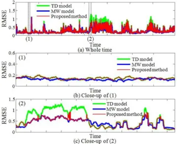
Three models were compared as follows; 1. Using only a TD model, 2. Using only a MW model, and 3. Using the proposed method. Figure 6 shows time plots of root mean square error (RMSE). Figure 6(a) was the prediction results of the three methods in the whole time. The horizontal axis was time and the vertical axis was RMSE that was criteria of predictive accuracy of statistical models. The proposed method could reduce the maintenance cost by 8.1% because the MW model was applied to 3,210 data of 39,515 data instead of the TD model. Figure 6(b) and (c) are close-ups of (1) and (2) in Figure 6(a). From Figure 6(b) it can be seen that when RMSE values of the TD model and MW model were almost at same levels, those of the proposed method were close to those of the TD model. This result suggested that the proposed method could keep high predictive ability re-ducing maintenance cost. Figure 6(c) shows that when RMSE values of the TD model were large, those of the proposal method were close to those of the MW model. This result suggested that the discriminant model detected the time when the state of the plant was different from the past operat-ing conditions under which the TD model was constructed. Then, a MD model was used instead of a TD model for pre-Table 1. The process variables of distillation column
Symbol Objective variable A Bottom product concentration No. Symbol Explanatory variables
1 F1 Reflux flow
2 F2 Reboiler flow
3 F3 Feed 1 flow
4 F4 Feed 2 flow
5 F5 Bottom flow
6 F6 Top flow
7 L1 Liquid level
8 P1 Pressure 1
9 P2 Pressure 2
10 T1 Temperature 1
11 T2 Temperature 2
12 T3 Temperature 3
13 T4 Temperature 4
14 T5 Bottom temperature
15 T6 Feed 1 temperature
16 T7 Feed 2 temperature
17 T8 Top temperature
18 F4/F3=R Reflux ratio 19 F1/F6=F Feed flow ratio
Table 2. The DR and the AR with the four methods
SVM PCA-SVM ICA-SVM EPM DRa (%) 47.7 55.9 58.0 77.3
ARb (%) 93.5 92.0 90.2 94.2
a : Detection ratio, b : Accuracy ratio.
Figure 6. Time plot of RMSE.
dicting the values of y. When RMSE values of a TD model were small, those of the proposed method were close to those of the TD model. It was conceivable that the MW model was affected by the data where the state of the plant was chang-ing from the process variation to the normal condition.
4. Conclusions
In this work, we developed the discriminant model considering the prediction error of a TD model for high pre-dictive ability and reduction of maintenance cost. The dis-criminant model judges whether a TD model is reliable in the current operating conditions or not. Through the analysis of the real industrial data, we concluded that the proposed method could reduce maintenance cost and improve pre-dictive accuracy of soft sensors. The proposed system will perform effective operations in chemical plants.
Acknowledgements
The authors acknowledge the support of Mizushima works, Mitsubishi Chemical Corporation.
References
Bersimis, S. Psarakis, S. and Panaretos, J. 2007. Multivariate Statistical Process Control Charts: An Overview. Qual-ity and ReliabilQual-ity Engineering International. 23, 517-543.
Comon, P. 1994. Independent component analysis, A new concept? Signal Processing. 36, 287-314.
Jolliffe, I.T. 1986. Principal Component Analysis. Springer-Verlag, New York, U.S.A.
Kadlec, P. Gabrys, B. and Strandt, S. 2009. Data-driven Soft Sensor in the process industry. Computers and Chemi-cal Engineering. 33, 795-814.
Kadlec, P. Grbic, R. and Gabrys, B. 2011. Review of adapta-tion mechanisms for data-driven soft sensors. Com-puters and Chemical Engineering. 35, 1-24.
Kaneko, H., Arakawa, M. and Funatsu, K. 2009. KAGAKU KOGAKU RONBUNSHU. 35, 382-389 (in Japanese). Kaneko, H. and Funatsu, K. 2011. Maintenance-Free Soft
Sensor Models with Time Difference of Process Vari-ables. Chemometrics and Intelligent Laboratory Systems. 107, 312-317.
Kaneko, H. and Funatsu, K. 2011. A Soft Sensor Method Based on Values Predicted from Multiple Intervals of Time Difference for Improvement and Estimation of Prediction Accuracy. Chemometrics and Intelligent Laboratory Systems. 109, 197-206.
Kano, M. and Nakagawa, Y. 2008. Data-based process moni-toring, process control and quality improvement: Recent developments and applications in steel indus-try. Computers and Chemical Engineering. 32, 12-24. Kourti, T. 2005. Application of latent variable methods to
process control and multivariate statistical process control in industry. Adaptive Control and Signal Pro-cessing. 19, 213-246.
Qin, S.J. 1998. Recursive PLS algorithms for adaptive data modeling. Computers and Chemical Engineering. 22, 503–514.
Appendix A
A support vector machine (SVM) is one of the classifi-cation methods used to generate nonlinear classifiers by ap-plying the kernel approach. In a linear SVM, the discriminant function f(x) is defined as follows:
x
Xw
b
f
(A-1)where x Rn (n represents the number of variables) denotes
a query sample, w Rn, a weight vector; and b, a bias. The
primal form of the SVM can be expressed as an optimization problem:
Minimize
i i
C
w2
2 1
(A-2)
subject to
,11 1
i
i i
i y
b w x
y
(A-3)
where yiand xirepresent training data; i, slack variables; and
C, the penalizing factor that controls the trade–off between a training error and a margin. By minimizing (A-2), a discri-minant model is constructed that shows a good balance between the ability to adapt to the training data and the ability to generalize. In our application, a kernel function is a radial basis function:
2
exp
,x x x
x
K