17
2017
REPORT OF THE WORKSHOP ON
SAMPLING EFFORT FOR BIOLOGICAL
PARAMETERS (WKSEBP)
Cristina Silva, Manuela Azevedo, Corina Chaves,
Rui Coelho, Ana Maria Costa, David Dinis, Sandra
Dores, Ana Cláudia Fernandes, Patrícia Gonçalves,
Pedro G. Lino, Hugo Mendes, Teresa Moura,
Cristina Nunes, Melinda Oroszlányová, Daniel
RELATÓRIOS CIENTÍFICOS E TÉCNICOS DO IPMA – SÉRIE DIGITAL
Destinam-se a promover uma divulgação rápida de resultados de carácter científico e técnico,
resultantes da actividade de investigação e do desenvolvimento e inovação tecnológica nas áreas
de investigação do mar e da atmosfera. Esta publicação é aberta à comunidade científica e aos
utentes, podendo os trabalhos serem escritos em Português, Francês ou Inglês.
Edição
IPMA
Rua C – Aeroporto de Lisboa
1749-007 LISBOA
Portugal
Corpo Editorial
Francisco Ruano – Coordenador
Aida Campos
Irineu Batista
Lourdes Bogalho
Mário Mil-Homens
Rogélia Martins
Teresa Drago
Edição Digital
Anabela Farinha
As instruções aos autores estão disponíveis no sitio web do IPMA
http://ipma.pt
ou podem ser solicitadas aos membros do Corpo Editorial desta publicação
Capa
Conceição Almeida
ISSN
2183-2900
Workshop on Sampling Effort for
Biological Parameters - WKSEBP
Citation:
Report of the Workshop on Sampling Effort for Biological Parameters
(WKSEBP)
Cristina Silva, Manuela Azevedo, Corina Chaves,
Rui Coelho, Ana Maria Costa, David Dinis, Sandra Dores,
Ana Cláudia Fernandes, Patrícia Gonçalves, Pedro G. Lino,
Hugo Mendes, Teresa Moura, Cristina Nunes,
Melinda Oroszlányová, Daniel Pinto and Maria do Carmo Silva
IPMA - Divisão de Modelação e Recursos da Pesca (DivRP) Av. Brasília, 1449-006 Lisboa
RESUMO
Título: Relatório do Workshop sobre o Esforço de Amostragem para a Estimação de Parâmetros Biológicos
O “Workshop on Sampling Effort for Biological Parameters (WKSEBP)”, presidido pelas investigadoras
Manuela Azevedo e Cristina Silva (IPMA), decorreu no IPMA-Algés, de 18 a 20 de Abril de 2017, para analisar o actual Programa Nacional de Amostragem Biológica (PNAB/Data Collection Framework) com o objectivo de otimizar o esforço de amostragem e melhorar a precisão na estimação de parâmetros biológicos. Foram analisados e discutidos vários métodos e abordagens que resultaram num conjunto de recomendações para trabalho futuro. Foram desenvolvidos quatro casos de estudo centrados nos seguintes temas: 1) amostragem de comprimentos em campanhas de investigação, 2) amostragem de comprimentos em lota, 3) estimação de chaves de idade-comprimento e 4) determinação de ogivas de maturação. Em cada caso de estudo foi analisado e discutido o número de amostras, o tamanho efetivo de cada amostra e a precisão na estimação dos parâmetros biológicos.
Palavras chave: amostragem por comprimentos, chave comprimento-idade, ogiva de maturação, tamanho efectivo da amostra.
ABSTRACT
The Workshop on Sampling Effort for Biological Parameters (WKSEBP), chaired by Manuela Azevedo and Cristina Silva (IPMA) met in Lisbon, 18 – 20 November 2017, to focus on the analysis of the current Portuguese sampling designs under PNAB/DCF (Programa Nacional de Amostragem Biológica/Data Collection Framework) with the aim to optimize the sampling effort and improve precision on the estimation of biological parameters. Several approaches and methodologies were discussed and guidelines for future work were recommended. Four case-studies were analyzed focusing on: 1) survey sampling for length, 2) at-market sampling for length, 3) estimation of age-length key and 4) maturity ogive. The number of samples, the effective sample size and the precision in parameters estimation were discussed in each case-study.
Key words: length sampling, age-length key, maturity ogive, effective sample size
REFERÊNCIA BIBLIOGRÁFICA
Table of contents
1 Introduction ... 7
1.1 Terms of reference ... 7
1.2 Background ... 7
1.3 Conduct of the meeting ... 7
1.4 Structure of the report ... 8
2 Case Study 1: Survey length sampling ... 9
2.1 Introduction ... 9
2.2 Methods ... 9
2.3 Results ... 11
2.4 Discussion and future work ... 18
2.5 References ... 19
3 Case Study 2: Hake at-market length sampling ... 20
3.1 Introduction ... 20
3.2 Analysis of data ... 22
3.3 Discussion and future work ... 27
3.4 References ... 28
4 Case Study 3: Blue-whiting age-at-length sampling ... 30
4.1 Introduction ... 30
4.2 Age-length Keys ... 30
4.3 Discussion and future work ... 39
4.4 References ... 40
5 Case Study 4: Mackerel and hake maturity ogive sampling... 41
5.1 Introduction ... 41
5.2 Maturity sampling ... 41
5.3 Maturity ogive estimation ... 43
5.4 Effective sample size and sampling variability on maturity ogive performance ... 44
5.5 Discussion and future work ... 49
5.6 References ... 50
6 Main Conclusions and Recommendations ... 53
Annex 1: List of participants ... 55
Annex 2: Meeting Agenda ... 56
1
Introduction
1.1 Terms of reference
The Workshop on Sampling Effort for Biological Parameters (WKSEBP), chaired by Manuela Azevedo and Cristina Silva met in Lisbon, 18–20 April 2017, to focus on the analysis of sampling effort needed to estimate biological parameters with a certain precision. Data used in the analysis were collected under PNAB/DCF (Programa Nacional de Amostragem Biológica/Data Collection Framework) and the main objective was to optimize the number of samples to collect, in terms of time and costs saving. Four case-studies were presented and analyzed during the workshop:
- CS 1) Surveys sampling for assessing the precision of length-frequency estimates: hake (Merluccius merluccius) and horse mackerel (Trachurus trachurus).
- CS 2) At-market sampling for landings length composition: hake commercial size categories.
- CS 3) Sampling for ALKs: blue-whiting (Micromesistius poutassou).
- CS 4) At-market sampling for maturity ogive: mackerel (Scomber scombrus) and hake.
1.2 Background
The Workshop was organized within the scope of the National Biological Sampling Programme - PNAB/DCF.
1.3 Conduct of the meeting
The workshop participants made available several sets of data and scripts prepared in advance to the meeting, as well as several presentations (Annex 4) which subsequently formed the basis of the
workshop’s investigations and discussions during the week.
The following speakers presented the talks indicated:
Case Study 1
P01 – Melinda Oroszlányová: Assessing the precision of length-frequency estimates (Following the paper of M. Pennington, 2002)
Case Study 2
P02 – Manuela Azevedo: At-market sampling for landings length composition: hake commercial size categories case-study. M. Azevedo, C. Silva
Case Study 3
P03 – Patrícia Gonçalves: Sampling for ALKs – blue-whiting case-study
Case Study 4
P04 – Ana Maria Costa: Southern mackerel, Scomber scombrus, mature ogive. A. Costa, C. Nunes, M. C. Silva.
Subgroup 2 – Effective sampling size in at-market sampling for size-categories. Subgroup 3 – Sampling for ALKs.
Subgroup 4 – Sampling for maturity ogive.
1.4 Structure of the report
The structure of the report is as follows:
Section 2 describes the work developed during the workshop, related to CS 1.
Section 3 describes the work developed during the workshop, related to CS 2.
Section 4 describes the work developed during the workshop, related to CS 3.
Section 5 describes the work developed during the workshop, related to CS 4.
2
Case Study 1: Survey length sampling
2.1 Introduction
One way to predict the status of a fish stock is to conduct an at-sea survey directed to the stock of
interest. IPMA’s at-sea surveys collect data to estimate the abundance (and relative abundance) of fish stocks and the relative frequency of population characteristics such as length, age, etc. It is of great importance to have precise and unbiased estimates; at the focus of this section is the study of precision, in particular of length-frequency estimates.
The aim of the exercise conducted for Case Study 1 is to optimize the number of individuals that need to be measured at surveys in order to determine the structure of the population regarding its length composition. Pennington et al. (2002) assesses the precision of length-frequency distributions estimated from trawl-survey samples, and shows that the effective sample size estimated using Kish’s design effect (Cochran, 1977) can be much smaller than the currently applied sample size. Such an optimal sample size can be derived from data sets that satisfy certain criteria. The main assumption of Pennington et al. (2002) is that fish caught together (i.e. at a given survey station) tend to have more similar characteristics (e.g. length), than those caught randomly from the entire population. This would imply that fish caught together will contain less information about the population length distribution than fish sampled randomly from the general population. In this case, the effective sample size for the estimate of the population length-frequency distribution could be much smaller than the number of fish sampled with the current design. In other words, the sample mean estimated from randomly measured fish from the population should have the same precision as the population mean estimated from fish measured with the currently applied method.
The objective of the present study is to estimate the effective sample size and test for the precision of mean length estimates, based on the methodology of Pennington et al. (2002), using data of two species, the European hake - Merluccius merluccius (HKE) and the Atlantic horse mackerel – Trachurus trachurus (HOM), from the Portuguese Bottom Trawl Surveys.
2.2 Methods
In order to estimate the optimal sample size defined by Pennington et al. (2002), first, one needs to estimate the variance of the population length distribution and the variance of population mean length. If fish are randomly sampled (or if all fish are sampled) at each station , and is the total number of fish caught during the survey (where is the actual or estimated number of fish caught at station ) and the length of the th fish at station , the variance of the
population length distribution can be estimated using the following expression:
.
(2.1)
In the above formula, is the ratio estimator of the population mean length of Cochran (1977), given as
, (2.2)
where is the estimate of the average length of fish caught at station .
where . Pennington et al. (2002) derives the estimate of the effective sample size by substituting (2.1) and (2.3) in
. (2.4)
As Pennington et al. (2002) relates the effective sample size to Kish’s design effect as follows:
, (2.5)
where is the number of fish sampled at random from the population, it can be written in the following form:
. (2.6)
Thus, , and so
. (2.7)
Then, by selecting random samples from the total number of fish caught, and comparing the mean length estimated from these samples with the population mean length estimated by using (2.2), one can assess the precision of mean length estimates.
The case study of the present section considers Portuguese Autumn Groundfish Surveys (PT-PGFS Q4) carried out by IPMA in the past two years (2015 and 2016), and uses the data of HKE and HOM,
to show whether Pennington’s method to determine the optimal number of individuals to be sampled at surveys can be adopted.
The survey area is the Portuguese continental coast, covering the area extending from latitude 41°20' N to 36°30' N (ICES Area IXa), where 12 sectors are defined along the three main geographical zones as follows:
i. North (N): Caminha (CAM), Matosinhos (MAT), Aveiro (AVE), Figueira da Foz (FIG), Berlengas (BER);
ii. Southwest (SW): Lisbon (LIS), Sines (SIN), Vila Nova de Milfontes (MIL), Arrifana (ARR); iii. South (S): Sagres (SAG), Portimão (POR), Vila Real de Santo António (VSA).
All of the above 12 sectors are further stratified by depth (1: ≤ 100m; 2: >100 and ≤ 200m; 3: >200 and ≤
500m), defining the strata. The data used for the analyses consist, for each sampled station, of the number of fish caught, their average length, the number of fish measured, and the estimated or actual length of every fish caught. For each station, information on zone, sector and stratum were also made available.
levels). While analyzing the above scenarios, several questions and doubts popped up, which are discussed below (see Section 2.4).
In order to show that the estimates obtained from fish sampled at random have the same precision of the sample mean obtained from the estimate based on the existing survey samples, 100 simulated distributions of for the different scenarios have been analyzed. The simulated estimates of the mean lengths were generated by randomly sampling (without replacement), from the total number of fish caught, a number of fish determined by the effective sample size formula (2.7).
2.3 Results
2.3.1 Exercise 1- Considering the whole survey region, without taking into account any
strata
2.3.1.1 Estimating the effective sample size
Table 2.1 presents the estimates of the effective sample size (denoted by ess_1) and summary statistics for assessing the precision of the estimated length distributions of HKE and HOM by year. When considering the whole survey region, the results indicate that for both HKE and HOM, the estimated effective sample size is very small compared to the number of sampled fish. This means that measuring only 1.5% of the samples in average would be sufficient in order to have the same precision of mean length estimates. The effective sample size per station was also calculated, however, its usefulness in this context, and whether it can be determined in such way is doubtful and discussed below (see Section 2.4).
Table 2.1. Data available and results for exercise 1 (considering the whole survey region, without taking into account any strata). See section 2.2 for further definitions.
Year Species Nº stations Nº fish (total) Nº sampled fish Rˆ (cm) var
(Rˆ)
2
ˆx
σ ess_1 ess_1/Nº stations
(ess_1/sampled fish)*100%
2015 HKE 83 21950 10733 19.9 0.1 36.1 263 3 2.5%
2016 HKE 81 7290 5078 22.3 1.4 71.6 51 1 1.0%
2015 HOM 66 72808 6356 14.9 0.7 30.9 47 1 0.7%
2016 HOM 55 11248 2580 19.0 0.2 10.4 44 1 1.7%
2.3.1.2 Re-sampling
Figure 2.1. Results from the resampling simulations and respective mean for hake (top) and horse mackerel (bottom), for the years 2015 (left) and 2016 (right).
2.3.2 Exercise 2 – Considering the survey region stratified by sectors
2.3.2.1 Rationale
The mean length varies with sector in both species (Figures 2.2 and 2.3), being most evident for horse mackerel (Figure 2.3). For this reason, it was hypothesized that length distributions could be more precisely defined if an effective sample size was estimated by sector.
Figure 2.2. Interquartile range of hake total length (cm) by sector in 2016.
HKE, 2015 HKE, 2016
HOM, 2015 HOM, 2016
mean(rs100) = 19.93217 mean(rs100) =22.32725
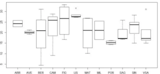
Figure 2.3. Interquartile range of horse mackerel total length (cm) by sector in 2016.
2.3.2.2 Estimating the effective sampling size
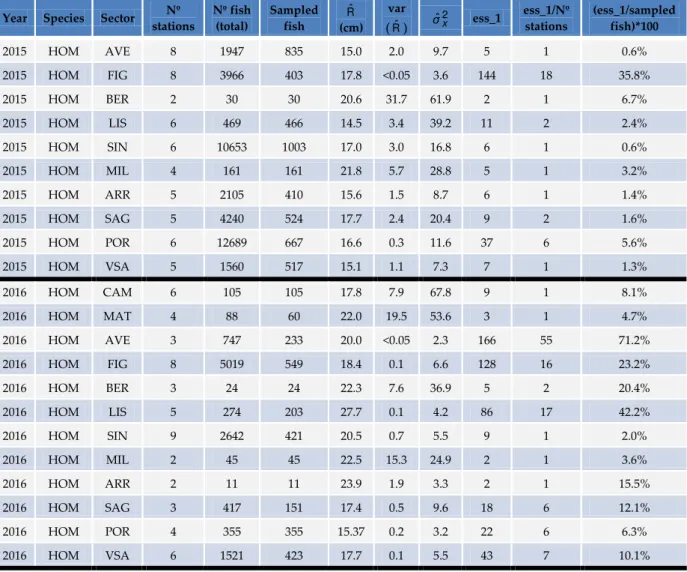
Table 2.2 contains the estimates of the effective sample size and summary statistics for assessing the precision of the estimated length distributions of HKE and HOM by sector, for each analyzed year. The results indicate that, similarly to exercise 1, the estimated effective sample size by sector is very small compared to the number of sampled fish, for both species. In the case of horse mackerel, very low effective sample sizes were estimated for some sectors despite the wide length range observed.
Table 2.2. Data available and results for exercise 2 (considering the survey region stratified by sectors). See section 2.2 for further definitions.
Year Species Sector Nº stations Nº fish (total) Sampled fish Rˆ (cm) var
(Rˆ)
2
ˆx
σ ess_1 ess_1/Nº stations
(ess_1/sampled fish)*100
2015 HKE CAM 8 3735 1412 20.7 0.3 30.1 113 14 8.0%
2015 HKE MAT 7 5197 1094 19.0 0.5 30.5 65 9 5.9%
2015 HKE AVE 7 1675 918 19.9 0. 8 14.1 18 3 2.0%
2015 HKE FIG 10 3308 2081 20.0 0.5 24.7 51 5 2.4%
2015 HKE BER 6 1619 890 21.1 2.2 26.6 12 2 1.4%
2015 HKE LIS 7 1220 862 17.5 0.5 29.4 54 8 6.3%
2015 HKE SIN 8 927 811 19.2 4.2 100.6 24 3 3.0%
2015 HKE MIL 6 594 594 18.8 3.6 66.3 18 3 3.1%
2015 HKE ARR 5 338 338 18.2 3.1 54.2 18 4 5.2%
2015 HKE SAG 5 455 354 24.5 0.7 61.1 86 17 24.3%
2015 HKE POR 7 1544 494 21.4 0.4 21.2 51 7 10.4%
2015 HKE VSA 7 1339 855 20.1 8.9 78.7 9 1 1.0%
2016 HKE CAM 8 799 676 26.1 0.6 41.5 73 9 10.8%
2016 HKE MAT 8 128 126 25.8 8.0 65.6 8 1 6.5%
2016 HKE AVE 5 109 109 24.7 5.5 36.4 7 1 6.1%
2016 HKE FIG 9 506 506 22.8 0.9 40.5 46 5 9.1%
2016 HKE BER 5 668 436 21.8 3.2 71.1 22 5 5.1%
2016 HKE LIS 9 986 769 21.5 1.3 51.6 40 5 5.3%
2016 HKE SIN 10 506 455 26.0 2.5 71.3 29 3 6.3%
2016 HKE MIL 4 368 368 19.8 5.5 69.9 13 3 3.5%
2016 HKE ARR 3 214 214 18.4 8.9 47.7 5 2 2.4%
2016 HKE SAG 5 167 123 24.3 2.1 78.5 38 8 31.0%
2016 HKE POR 8 1499 544 16.8 4.6 83.2 18 2 3.4%
Year Species Sector Nº stations Nº fish (total) Sampled fish Rˆ (cm) var
(Rˆ)
2
ˆx
σ ess_1 ess_1/Nº stations
(ess_1/sampled fish)*100
2015 HOM AVE 8 1947 835 15.0 2.0 9.7 5 1 0.6%
2015 HOM FIG 8 3966 403 17.8 <0.05 3.6 144 18 35.8%
2015 HOM BER 2 30 30 20.6 31.7 61.9 2 1 6.7%
2015 HOM LIS 6 469 466 14.5 3.4 39.2 11 2 2.4%
2015 HOM SIN 6 10653 1003 17.0 3.0 16.8 6 1 0.6%
2015 HOM MIL 4 161 161 21.8 5.7 28.8 5 1 3.2%
2015 HOM ARR 5 2105 410 15.6 1.5 8.7 6 1 1.4%
2015 HOM SAG 5 4240 524 17.7 2.4 20.4 9 2 1.6%
2015 HOM POR 6 12689 667 16.6 0.3 11.6 37 6 5.6%
2015 HOM VSA 5 1560 517 15.1 1.1 7.3 7 1 1.3%
2016 HOM CAM 6 105 105 17.8 7.9 67.8 9 1 8.1%
2016 HOM MAT 4 88 60 22.0 19.5 53.6 3 1 4.7%
2016 HOM AVE 3 747 233 20.0 <0.05 2.3 166 55 71.2%
2016 HOM FIG 8 5019 549 18.4 0.1 6.6 128 16 23.2%
2016 HOM BER 3 24 24 22.3 7.6 36.9 5 2 20.4%
2016 HOM LIS 5 274 203 27.7 0.1 4.2 86 17 42.2%
2016 HOM SIN 9 2642 421 20.5 0.7 5.5 9 1 2.0%
2016 HOM MIL 2 45 45 22.5 15.3 24.9 2 1 3.6%
2016 HOM ARR 2 11 11 23.9 1.9 3.3 2 1 15.5%
2016 HOM SAG 3 417 151 17.4 0.5 9.6 18 6 12.1%
2016 HOM POR 4 355 355 15.37 0.2 3.2 22 6 6.3%
2016 HOM VSA 6 1521 423 17.7 0.1 5.5 43 7 10.1%
2.3.2.3 Re-sampling
The re-sampling simulations showed that the means had values close to Rˆ. Figure 2.4 illustrates the results of resampling for hake and horse-mackerel in sector CAM.
Figure 2.4. Results from the re-sampling simulations and respective mean for hake and horse mackerel in sector CAM in 2015.
HKE HOM
2.3.3 Exercise 3 – Considering the survey region stratified by zones ( N, SW and S) and by depth (3 levels)
2.3.3.1 Rationale
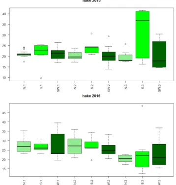
Mean lengths vary with sector, but also with depth (Figures 2.5 and 2.6). For these reasons, it was also tested whether length distributions could be more precisely defined when an effective sample size is estimated by area and stratum.
Figure 2.5. Interquartile range of hake total length (cm) by area and stratum in 2015 and 2016.
2.3.3.2 Estimating the effective sample size
When stratifying the survey region, the optimal sample sizes for the estimates of the length composition of HKE followed the same pattern, with proportions from the samples that would be sufficient to measure varying between 0.8% and 26.2%. In the case of HOM, the results show a different pattern, with more extreme effective sample size estimates in certain strata, reaching 733.3% of the sampled fish that should be measured. It might be due to negative intra-haul correlation, what can push the effective sample size above the number of fish sampled (Cochran, 1977). Although, this is rare for trawl surveys (Pennington et al., 2002).
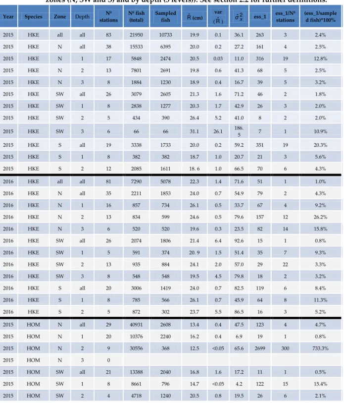
Table 2.3. Data available and results for exercise 3 (Considering the survey region stratified by zones (N, SW and S) and by depth (3 levels)). See section 2.2 for further definitions.
Year Species Zone Depth stationsNº Nº fish (total) Sampled fish Rˆ(cm) var
(Rˆ) 2
ˆx
σ ess_1 ess_1/Nº
stations
(ess_1/sample d fish)*100%
2015 HKE all all 83 21950 10733 19.9 0.1 36.1 263 3 2.4%
2015 HKE N all 38 15533 6395 20.0 0.2 27.2 161 4 2.5%
2015 HKE N 1 17 5848 2474 20.5 0.03 11.0 316 19 12.8%
2015 HKE N 2 13 7801 2691 19.8 0.6 41.3 68 5 2.5%
2015 HKE N 3 8 1884 1230 18.9 0.4 16.7 39 5 3.2%
2015 HKE SW all 26 3079 2605 21.3 1.6 71.2 46 2 1.8%
2015 HKE SW 1 8 2838 1277 20.3 1.7 42.9 26 3 2.0%
2015 HKE SW 2 5 434 390 26.4 5.2 41.0 8 2 2.0%
2015 HKE SW 3 6 66 66 31.1 26.1 186.
5 7 1 10.9%
2015 HKE S all 19 3338 1733 20.0 0.2 59.2 351 19 20.3%
2015 HKE S 1 8 382 382 18.7 1.0 20.7 21 3 5.6%
2015 HKE S 2 12 2085 1611 18. 6 1.0 66.5 70 6 4.3%
2016 HKE all all 81 7290 5078 22.3 1.4 71.6 51 1 1.0%
2016 HKE N all 35 2211 1853 24.0 0.7 54.9 79 2 4.3%
2016 HKE N 1 16 857 734 26.1 0.5 33.7 67 4 9.2%
2016 HKE N 2 13 834 599 24.6 0.5 79.6 157 12 26.2%
2016 HKE N 3 6 520 520 19.6 0.3 23.5 82 14 15.8%
2016 HKE SW all 26 2074 1806 21.4 6.4 92.6 15 1 0.8%
2016 HKE SW 1 5 591 374 20. 9 1.5 51.4 35 7 9.3%
2016 HKE SW 2 13 935 884 24.1 2.0 57.0 29 22 3.3%
2016 HKE SW 3 8 548 548 19.5 4.5 79.8 18 2 3.2%
2016 HKE S all 20 3006 1419 24.0 0.7 82.5 119 6 8.4%
2016 HKE S 1 8 785 566 26.1 0.7 45.9 64 8 11.3%
2016 HKE S 2 5 872 302 23.7 5.5 86.5 16 3 5.2%
2015 HOM N all 29 40931 2608 13.4 0.4 47.5 123 4 4.7%
2015 HOM N 1 20 10376 2240 16.2 0.4 6.9 19 1 0.8%
2015 HOM N 2 9 30556 368 12.5 <0.05 65.6 2699 300 733.3%
2015 HOM N 3 0
2015 HOM SW all 21 13388 2040 16.8 1.6 17.2 11 1 0.5%
2015 HOM SW 1 8 8661 796 14.7 <0.05 4.2 122 15 15.4%
Year Species Zone Depth Nº
stations
Nº fish (total)
Sampled
fish Rˆ(cm)
var
(Rˆ) 2
ˆx
σ ess_1 ess_1/Nº
stations
(ess_1/sample d fish)*100%
2015 HOM SW 3 4 7 4 25.1 14.6 62.2 4 1 107.5%
2015 HOM S all 16 18489 1708 16.7 0.3 13.8 41 3 2.4%
2015 HOM S 1 8 7004 1174 18.1 0.6 14.4 23 3 2.0%
2015 HOM S 2 11 11443 492 15.8 0.1 11.0 83 8 16.8%
2015 HOM S 3 2 42 42 27 6.3 28.7 5 2 11.0%
2016 HOM all all 55 11248 2580 19.0 0.2 10.4 44 1 1.7%
2016 HOM N all 24 5983 971 18.6 0.2 8.4 50 2 5.1%
2016 HOM N 1 14 5863 879 18.5 0.1 6.6 72 5 8.1%
2016 HOM N 2 8 115 87 27.2 1.0 15.8 17 2 19.1%
2016 HOM N 3 2 5 5 31.9 0.1 0.8 14 7 278.0%
2016 HOM SW all 18 2293 680 21.2 1.0 10.0 10 1 1.5%
2016 HOM SW 1 6 2391 398 20.2 0.5 5.8 11 2 2.9%
2016 HOM SW 2 11 570 271 25.3 0.6 4.7 7 1 2.7%
2016 HOM SW 3 1 11 11 31.6 2.5 0 0.0%
2016 HOM S all 13 2973 929 17.3 0.1 6.6 71 6 7.7%
2016 HOM S 1 8 711 487 17.1 0.6 12.3 22 3 4.4%
2016 HOM S 2 3 422 278 16.6 0.2 2.6 11 4 3.8
2.3.3.3 Resampling
Figure 2.7. Results from the resampling simulations and respective mean for horse mackerel in 2016 by area: North, North per station, North1, North1 per station, North2 and North2 per station.
2.4 Discussion and future work
Three main types of exercises have been conducted regarding survey fish length sampling. The first one focuses on estimating the optimal sample size for one species at a time per survey. Since the number of stations at the surveys might vary from year to year, as well as the total number of fish caught and the number of fish sampled, it means that the optimal sample size may also vary from year to year. Thus, it might not be enough to estimate the effective sample size only from one year and apply it for future years, but it shall be estimated from a group of surveys of the same type. Therefore, it might be preferred to estimate the optimal sample size for instance for the last few years (at least 5-10), and calculate their average. Then, this average optimal sample size could be used as a reference at the forthcoming surveys.
N N per station
N1 N1 per station
N2 N2 per station
mean(rs100) = 18.6284 mean(mN24_100) =22.40
mean(rs100) = 18.44236 mean(mN1_100) =19.38043
The abundance of a particular species in a survey region can be variable. This motivated the second type of exercise, in which the optimal sample size was estimated for each of the 12 pre-defined sectors
(“water cuboids”) along the Portuguese coast. Such stratification might imply that the estimated
optimal sample size can be much smaller or much greater in some sectors than the estimated optimal sample size without stratifying the data per sectors. Similarly, the third type of exercise, where the survey area is divided into three major zones (N, SW and S) with three depth strata in each, faces the same implications of stratifying the survey region.
The question is: which method is the best to determine the optimal sample size for a particular group (cluster) of fish, i.e. per station. While looking for the answer, one has to keep in mind that, as Pennington et al. (2002) reminds, besides variable fish density, very small effective sample sizes, and so rather imprecise estimates of length distributions might be due to fish being more similar in a haul, i.e., at a station, than fish in the general population. If fish of similar length tend to be caught together, with the increased variance, the effective sample size can drastically decrease (because of intra-haul correlation, see Cochran, 1977).
A very low effective sample size per station implies that in order to significantly improve survey precision, fish should be sampled from as many locations as possible. This could improve overall survey efficiency without increasing survey cost. If more locations were sampled (with shorter hauls), the total number of fish caught would be less in average, but the estimates of fish density (abundance) would be more precise, and the resulting fish samples would be more representative of the whole population. However, changing survey design accordingly could lead to the loss of information for less abundant species.
For some species it might be preferred to stratify the catch at a station, e.g. for small, medium and large size categories. In this case, a random sample would be chosen from each stratum, and the stratified mean length ( ) would be estimated. For other sampling schemes at a station, the variance of the population length distribution is calculated differently from (1), based on the frequency of fish in each length bin ( ) and the bins’ midpoints ( ):
.
(2.8)
Further investigation should be performed to explain the extreme effective sample size estimates observed for HOM in certain strata (exercise 3) and to evaluate whether length distributions could be more precisely defined. Future work is also needed to check whether this methodology can be applied to all species, considering fish distribution patterns. Finally, the influence of the change in the sampling effort (using effective sample size) on the raising procedure and on the estimation of the total length composition should be evaluated.
2.5 References
Cochran WG, 1977. Sampling techniques. 3rd ed. John Wiley and Sons, New York, NY, 428 p.
3
Case Study 2: Hake at-market length sampling
3.1 Introduction
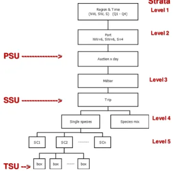
The current at-market sampling design is a stratified multistage design, with [auction * day] as the Primary Sampling Unit (PSU). It is stratified by fleet (or métier), auction and quarter (Figure 3.1). Following the DCF requirements (EU, 2016a), less significant fleets are not sampled (e.g. dredges, beach-seines) and sampling effort is based on number of trips. Annual sampling effort is fixed by the DCF National Sampling Plan (EU, 2016b) which sets the number of trips to be sampled for each fleet
(≈ métier). Sampling effort is allocated to auctions and quarters proportionally to the most recent
year’s landings.
For each fleet, the visit dates in each [auction * quarter] are spread somewhat systematically throughout the quarter in a way that covers all week days of that fleet activity.
In every [auction * visit_date], observers attempt to sample a predefined number of vessel sale events, which are haphazardly selected from a list of all landings awaiting auction. This list includes the name of each vessel and the commercial species, commercial category and weight of each of landed box. Each vessel sale event generally corresponds to the landings of one fishing trip. A minor proportion of vessel sale events may not be present in the selection list when sampling starts.
From each selected trip, the observers aim to sample boxes from every landed species and commercial size category. Within each size category, the observers select 1 box randomly. Since 2014, when there are very few fish from a species inside the box, observers take more boxes until the length composition of the size category is well defined. Also, when different species are present within a box, observers sample them all. This sampling design, referred to as “trip-based” design, is linked to the concurrent sampling.
Figure 3.1. Current at-market sampling design (Azevedo et al., 2016)
Some difficulties may constrain this sampling strategy, namely vessels arriving to port after the auction has started, with large amounts of landings/species/categories meaning no time to sample the complete trip. (e.g.: OTB_DEF). Also, some commercial species may not be available for sampling if they have previously been included in a fixed sale contract. Sometimes, when observers do not have time to sample all commercial species, the more important species (for stock assessment, with TAC, etc) are selected.
The aim of this case-study is to analyze the effective sampling size to estimate the annual length composition of hake landings, based on the length distribution by size category obtained from sampling size categories. Modeling length distribution using commercial size categories was first presented in the Workshop on Sampling Design and Optimization of (Azevedo et al., 2014), using horse-mackerel data and later its application in a horse mackerel focused pilot plan was further developed in Azevedo et al., 2016 and ICES, 2017. In this case-study, the sampling effort and the effective number of length measurements by sample in a size category sampling design for hake are discussed. This sampling design, referred herein after as “size category-based” design, is a “species
focus” sampling scheme.
The analysis was carried out based on the year 2013 sampling data. The main auction markets sampled were grouped in three zones: NW (Póvoa do Varzim, Matosinhos, Aveiro and Figueira da Foz); SW (Peniche, Sesimbra and Sines); and S (Portimão, Olhão and Vila Real de Santo António). In these ports, trips from several metiers were sampled, particularly bottom otter trawl trips targeting either demersal fish or crustaceans and trips from multi-gear vessels, some of them identified as using gill or trammel nets and longliners (P02).
The dataset comprises length data for hake, recorded in 365 sampled trips with hake landings (positive trips), corresponding to 720 samples and 5748 length measurements. Table 3.1 summarizes the total number of trips sampled, the number of samples and the number of individuals measured by size category and zone. In 2013, the maximum number of sampled hake individuals per size category box was around 30. There were, however, several sampled trips where the number of hake landed by size category was very low, especially in size categories that include the larger individuals (T1 and T2) (see Table 3.1).
The analyses were performed using the statistical environment R (R Core Team, 2017).
Table 3.1. Summary statistics of hake at-market sampling in 2013: total number of trips per zone, number of samples and number of individuals measured by zone and size category (SC).
zone SC # trips # samples # indiv
T1 39 184
T2 39 161
T3 54 373
T4 93 708
T5 48 325
Total 146 273 1751
T1 25 155
T2 32 257
T3 46 314
T4 57 441
T5 22 195
Total 106 182 1362
T1 16 76
T2 28 187
T3 78 814
T4 82 861
T5 61 697
Total 113 265 2635
TOTAL 365 720 5748
NW
SW
3.2 Analysis of data
3.2.1 Size categories (SC)
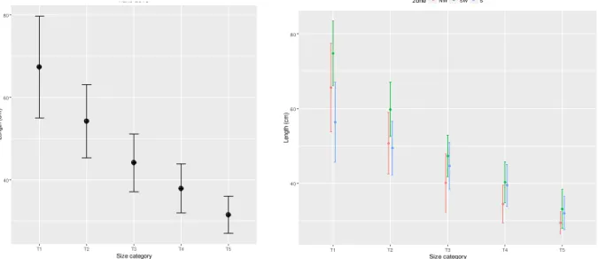
In the auction, landings of hake and of other species are sold in size categories. In the case of hake there are 5 size categories from T1 (largest fish) to T5 (smallest fish), which have different market prices. Although the size category classification is established by EU regulation (Council Regulation (EC) No. 2406/96 of 26 November 1996), its application may differ by zone. Figure 3.2 presents the 2013 hake landings by size category and zone. As shown, in 2013 the size categories with highest landings were T4 and T5 (small sizes) and mainly from the NW and SW. In S zone, low landings were recorded for the largest fish, T1 and T2. Figure 3.3 shows the overall mean length (± 1 sd) in each size category and its variability among zones for 2013.
Figure 3.2. Portuguese hake landings by size category and zone.
Figure 3.3. Mean length (± 1 standard deviation) by size category in 2013. Left – all samples combined; right – samples by zone.
40 60 80
T1 T2 T3 T4 T5
Size category L e n g th (c m )
zone NW SW S
40 60 80
T1 T2 T3 T4 T5
To estimate the required sampling effort (number of positive trips) to characterize the size categories,
two approaches, the “trip-based” and “size category-based” designs, were developed and described in the following sections. Given that the mean length by size category may vary among zones (Figure 3.3), the analyses were carried out considering this factor.
3.2.2 Trip-based design
The first set of analyses aimed at exploring the number of (positive) trips necessary to characterize the length composition by size category.
Considering that no major changes are made to the current trip sampling design, simulations were performed by zone, i.e. a number k of whole trips are randomly sampled in each zone and all the existing size categories and length measurements from each sampled trip were used for the analysis. It is noted that the trip landings may not include all size categories. The simulation scheme is presented in Figure 3.4.
Figure 3.4. Simulation scheme for the trip-based design 1. i– levels of zone; k– number of trips to sample; b– number of re-samples)
The simulations were performed with and without trip replacement for the three zones, with k = 10:100 (step 10) and 100 re-samples. As shown in Table 3.1, the number of trips with hake landings, sampled in 2013 in each zone (NW = 146, SW = 106, S = 113), is greater than the maximum value of k.
The expected number of samples by size category (minimum and maximum) and zone for the simulated k trips (Table 3.2) is below or well below the number of sampled trips in 2013, since not all size categories are landed in each trip and some size categories are less frequent in some zones.
zone i (NW, SW, S)
i = 1 to 3 sample k trips
k = 10 to 100 (step 10)
b = 1 to 100
k trips by zone
Table 3.2. Trip-based design. Minimum and maximum number of samples by size category and sampled trips (k from 10 to 100, step 10) in each zone, from simulations with 100 re-samples with replacement.
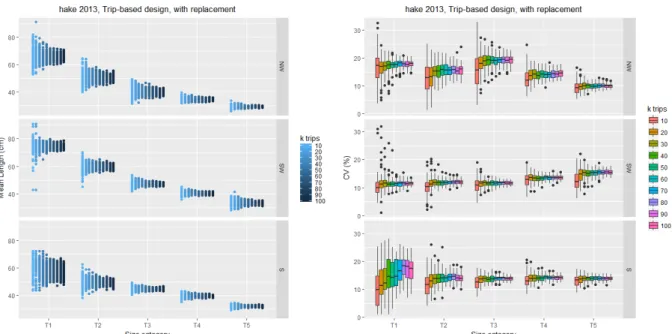
For each size category j in each zone i, the mean length, standard deviation (sd) and coefficient of variation (CV) were computed for each re-sample and k. As expected, the results are similar when sampling is carried out with or without replacement. Figure 3.5 shows the variability of the mean length and CV for the sampling with replacement.
For size categories T3, T4 and T5, which are the size categories with higher landings, the variability in the mean length does not change much for k ≥ 40 in all zones. The size categories T1 and T2 which have lower landings in the NW and S, show decreasing variability in the mean length, from 10 to 60 trips.
For k ≥ 40 the CVs were, on average, below 15% for all size categories in SW, for T2 to T5 in S and for T4 and T5 in NW. The highest CVs and variability was observed in T1 in S for k between 10 and 70 trips, which reflects the low number of samples of T1 in the dataset (Table 3.1).
Zone k T1 T2 T3 T4 T5 T1 T2 T3 T4 T5
10 0 0 0 3 0 6 5 7 9 7
20 0 1 2 6 0 9 10 12 17 12
30 3 3 3 14 4 15 13 18 25 18
40 3 5 9 18 6 18 18 24 33 21
50 7 5 11 24 7 21 21 27 41 25
60 8 10 14 27 13 24 26 29 47 31
70 9 10 15 34 14 33 34 35 53 35
80 12 14 15 43 17 31 32 42 61 38
90 13 13 25 44 19 38 33 44 66 39
100 17 12 26 51 21 43 38 48 79 45
10 0 0 1 1 0 5 6 9 8 7
20 0 1 4 6 0 10 11 15 16 9
30 2 3 7 8 2 14 15 19 22 11
40 4 6 10 13 2 16 20 29 28 16
50 6 8 10 17 3 18 25 30 35 17
60 6 5 15 21 5 22 29 35 43 24
70 8 14 22 28 6 25 36 42 47 22
80 10 16 24 32 8 32 33 44 53 30
90 12 18 26 36 9 32 39 50 63 29
100 11 18 28 43 12 34 45 54 66 29
10 0 0 2 4 2 4 6 10 10 10
20 0 0 9 8 5 7 9 19 20 16
30 0 2 14 15 11 9 14 28 26 21
40 1 5 19 22 12 12 17 35 35 30
50 2 5 28 29 20 13 20 45 45 35
60 3 8 30 35 24 16 22 50 52 43
70 3 9 40 38 24 20 26 58 60 47
80 5 9 44 46 34 18 28 64 66 53
90 5 13 52 56 37 21 32 73 75 60
100 8 13 58 53 41 22 34 82 82 66
Min Max
NW
SW
Figure 3.5. Trip-based design. Mean length (left) and length CV (right) by size category and number of sampled trips (k from 10 to 100, step 10) by zone, from simulations with 100 re-samples with replacement.
The second set of simulations aims to estimate the effective sample size (number of fish to be measured) by size category, to characterize its length distribution.
Considering the same trip-based design, how many fish shall we take from a size category in each sampling event to characterize its length distribution? In this case, sampling is performed in two steps: 1) the trips are sampled by zone as in the previous scheme, and 2) from each category of each sampled trip, n lengths are sampled. Considering the number of individuals that were measured from each trip/size category combination in the 2013 dataset ( 1 to 30), this second step was carried out with replacement. Again, as in the previous simulation, if one category is missing in the trip, this category will not be sampled. The simulation scheme is presented in Figure 3.6.
Figure 3.6. Simulation scheme for the trip-based design 2. i– levels of zone; k– number of trips to sample; j– size category levels; n– number of lengths to sample; b– number of re-samples.
Simulations were performed by zone for k = 40 trips (representing a reduction around 70% of the 2013 sampling effort, Table 3.1) and n from 4 to 16 fish (step 4). Since not all trips landed all size categories, the number of samples by size category for 40 trips varied according to Table 3.2, though the
zone i (NW, SW, S)
i = 1 to 3
size cat j (T1, ... T5)
j = 1 to 5 sample
k trips
k = 40
sample n lengths by sc from each trip
lengths by b, i, k, j, n
n = 4 to 16 (step 4)
b = 1 to 100
simulated number of fish measured in each size category sampled was achieved since the re-sample of n was performed with replacement.
The results indicate that the variability of the estimated mean length and its CV by size-category are very similar for all n analyzed, in each zone (Figure 3.7). However, as noted above, the achieved total sample size by size category and zone was well below the intended (i.e. 160 for n = 4, 320 for n = 8, 480 for n = 12 and 640 for n = 16).
Figure 3.7. Trip-based design. Mean length (left) and its CV (right) with number of sampled individuals n (# ind from 4 to 16, step 4) by size category and zone. Simulations for k = 40 trips by zone, with 100 re-samples with replacement.
3.2.3 Size category-based design
In this approach, the trips are ignored and for each zone and size category, s samples of size n are taken.
For the analysis the samples (fish lengths) may be obtained using two approaches:
i) Randomly generate the samples assuming a normal distribution characterized by the mean length and standard deviation by size category and zone;
ii) Randomly sample from a pool of all lengths measured in 2013 in each size category and zone.
Figure 3.8. Simulation scheme for the size category-based design. i) and ii) represent two different sampling procedures. i– zone levels; j– size category levels; s– number of samples: n– number of lengths to sample; b– number of re-samples.
As expected, both variants give similar results:
- Stable mean length within each [zone * size category] combination, no matter the size of n.
- No trend observed in CV with the increase of n in each [zone * size category] combination.
Figure 3.9 shows the results for the variant ii). Sampling only 4 fish by size category in 40 samples corresponds to 160 fish to be measured by zone and a total annual of 2400 fish (160 fish x 3 zones x 5 sc). The results suggest a reduction of around 60% in the number of fish measured in 2013 (Table 3.1).
Figure 3.9. Size category-based design. Mean length (left) and its CV (right) with number of sampled individuals n (# ind from 4 to 16, step 4) by size category. Simulations for 40 samples by zone, with 100 re-samples with replacement.
3.3 Discussion and future work
Considering the current trip-based sampling design, in the case of hake landings, the simulations using 2013 data suggest that the number of trips to be sampled, for the characterization of size categories length distributions, may be reduced to around 40 in each zone. Table 3.2 illustrates the minimum and maximum number of samples by size category and k, in each zone, for the simulations performed with 100 re-samples with replacement. For example, with k = 40 trips, there is a chance of
zone i (NW, SW, S)
i = 1 to 3
size cat j (T1, ... T5)
j = 1 to 5 s = 40
lengths by b, i, j, s, n
n = 4 to 16 (step 4)
b = 1 to 100
number of samples doubled, though it is still low (2 samples). The simulations for the effective sample size of length measurements (n) by size category were carried out considering the trip-based design (k = 40 trips) and the alternative size category-based design (s = 40 samples) from n = 4 to 16 fish. The size category-based design is not limited by the sampled trips, i.e. the current sampling level
“métier” and sampling unit “trip” (Figure 3.1) are removed. Although the size categories classification may show some variability among zones/ports, in the same auction market no differences among gears are expected.
The comparison of mean lengths and CV obtained from the two designs (see Figures 3.7 and 3.9) shows that the two designs have similar mean lengths per size category but the mean length has lower variability in almost all size categories with the size category-based design. This is due to the
fact that in a “size-category” sampling design observers will haphazardly select boxes by size category from a list of all boxes by size category awaiting auction. Therefore, in an auction visit, as the aim is not to sample a number of trips by métier but a number of individuals by size category, the probability of getting samples by size category increases. Also, if the number of individuals in a size category box is not enough, it is possible to complete the required number taking fish from another box, provided that more than one box of that category was landed. In the case of the trip-based design the observer will sample only the size categories present in the randomly selected trips (2 or 3 trips) and will be limited to the number of fish that is present in each size category box. If this number is low (e.g. T1), the size category may present larger variability of the mean length.
Even though the results from the size category approach suggest that n = 4 fish would provide reasonable precision levels for the mean length of the most representative size categories, the analysis should be extended to other years to investigate the consistency in the variability of the mean length by size category within and among zones, before its implementation.
Moreover, the analysis should also look at the required number of [auction * visits] by zone to accomplish either k = 40 trips (trip-based design) or s = 40 samples by size category (size category-based design). In the first case, it means computing the probability of trips with hake landings in an auction day and, for a positive trip, the probability of occurrence of each size category in the landings of hake; in the second case, taking into account the probability of occurrence of each hake size category in an auction day. Decision on the number of samples by size category will be a trade-off between accepted levels of precision and costs associated. For example, in 2013 the landings of T1 in zone S were low and the lowest among zones. This means that achieving s = 40 in T1 in S would likely require an enormous number of [auction * visits] with unacceptable sampling costs and without significantly improving the precision of the annual landings length composition.
It is recommended to perform another type of analysis with prior definition of acceptable precision levels (e.g. CV ≤ 12%) for the more represented size categories in landings. The maximum number of samples and required [auction * visits] by zone to accomplish the target precision (e.g. in NW: s = 30 for T4 and s = 20 for T5, hence, maximum = 30) will be used to compute the precision of the less represented categories in the landings (T1, T2 and T3). Our results suggest that, in this case, the precision of the less represented size categories in landings will be ≥ 20% CV, which may well be acceptable given the low contribution of the landings of these size categories to the total landings length composition.
3.4 References
Azevedo M, Silva C, Vølstad JH, 2016. Modelling length distribution by commercial size category to estimate species catch length composition for stock assessment. ICES Annual Science Conference, Riga – Latvia, 19-23 September 2016. ICES CM 2016/O:170.
EU, 2016a. Commission Implementing Decision (EU) No. 2016/1251 of 12 July 2016 adopting a multiannual Union programme for the collection, management and use of data in the fisheries and aquaculture sectors for the period 2017-2019. Official Journal of the European Union L 207: 113 – 177. EU, 2016b. Commission Implementing Decision (EU) No. 2016/1701 of 19 August 2016 laying down rules on the format for the submission of work plans for data collection in the fisheries and aquaculture sectors. Official Journal of the European Union L 260: 153 – 228.
ICES. 2017. Report of the Working Group on Commercial Catches (WGCATCH), 7-11 November 2016, Oostende, Belgium. ICES CM 2016/SSGIEOM:03. 142 pp.
4
Case Study 3: Blue-whiting age-at-length sampling
4.1 Introduction
Estimating ages from hard structures for a large number of fish is very time-consuming, whereas measuring the length of a large number of fish is usually relatively faster and simple. The age structure for a large number of fish can be estimated by the relationship between age and length for a relatively small subsample of fish and then applying an age-length key (ALK) to the entire sample of fish. The selection of the subsamples to be used to construct the age-length key could be random (i.e. the number of specimens aged from each length category proportional to the number in each length category) or fixed (i.e. a constant number of specimens aged from each length category) (Kimura, 1977). Currently, the most common method of subsampling is to create length-groups of 10-mm, 25-mm, or 1mm lengths and collect age data structures from a fixed number of fish per length-group. The ages of fish in the subsample are then estimated by various methodologies, and statistics such as mean length and variance are computed for each age group represented in the subsample (Betolli and Miranda, 2001).
In most of the cases, a major problem is to achieve the exact fixed number of fish aged by length, in order to guarantee a compromise between the time-spent ageing and the final data quality on the ALKs. Due to the difficulty on comparing and assessing ALKs quality, the evaluation of age-length estimates is usually done based on the growth models. In fisheries, the most widely used growth model is the von Bertalanffy model, derived in 1938 by von Bertalanffy and based on simple physiological arguments. This model assumes that the growth rate of a fish declines with size, the change in the fish growth rate (dl/dt) is described by (Eq. 4.1):
(4.1)
where t is time, l is length, K is the growth rate and L is the asymptotic growth at which growth is zero. The von Bertalanffy growth model equation (Eq. 4.2) is given by integrating equation 4.1. and described as:
(4.2)
The main goal of this case study was to develop an algorithm to define the minimum fixed number of fish by length class that should be used to construct the age-length key. Length and age data (determined from otolith readings) for blue-whiting (Micromesistius poutassou) from year 2004 and 2008 were used as test cases.
The algorithm, the statistical analyses and the plots were performed using the statistical environment R (R Core Team, 2017).
4.2 Age-length Keys
4.2.1 Ageing sampling procedure
Figure 4.1. Number of blue-whiting otoliths collected (red) and aged (blue) by year, from 2000-2016, for the Portuguese coast. The green rectangles show the transition in the total number of aged otoliths: before 2011, all the collected were aged; after 2011, a random sample of 10 by length-class and quarter were aged.
4.2.2 Simulations
The following sampling scenarios were tested: the sampling period (quarter, semester, year) (Section 4.2.2.1) and the fixed number of otoliths to read by length class (1, 2, 4, 5, 10, 20, 30, 40, 50, 100) (Section 4.2.2.2).
4.2.2.1 Periodicity
The blue-whiting sampling data from 2004 were used to test whether the fixed number of 10 otoliths by length class (5 males and 5 females) uniformly distributed by port, should be collected by quarter (the current sampling scheme), by semester or by year. A total of 100 sampling simulations, without replacement, were performed in order to test each of those scenarios.
Figure 4.2. Number of blue-whiting otoliths aged by length class (cm) in 2004 (in total n=907).
The 2004 ALK representation is shown in Figure 4.3.
The von Bertalanffy growth model (4.2) was fitted to the age-length data obtained from the random sampling of 10 aged otoliths by length class (1 cm) and by quarter, by semester and by year and compared with the growth curve considering all the otoliths aged in 2004 (all) (Figure 4.4).
Figure 4.4. Blue-whiting growth curves from fitting von Bertalanffy growth model to all the 2004 data (red) (original data) and simulated samples of 10 otoliths by length class, using year (green), semester (blue) and quarter (violet) based selection. X-axis represents age and Y-axis represents length (cm).
The curves obtained by sampling a fixed number of otoliths selected by quarter and by semester were similar and also close to the curve when using all otoliths collected/read in 2004.
Figure 4.5. Blue-whiting length distribution by age from the 100 simulations (Simulation (ID)) of 10 otoliths per length class based on quarter, semester and annual sampling, and with all the 2004 available data (original data).
Figure 4.6. The parameters (Linf (a), k (b) and t0 (c)) from the von Bertalanffy growth model fitted to the 10-otoliths by length class data simulations, based on year (orange), semester (green) and quarter (blue) selection.
The figures above reveal similarities between the parameters obtained based on a quarterly and semester selection. Taking into account, the scenario of achieving the minimum number of aged fishes, the results support the change to the semester-based sampling period.
4.2.2.2 Number of otoliths by length class
The semester was then used as a base for testing the number of otoliths to read by length class, according to the results of the previous section (Section 4.2.2.1). The Portuguese blue-whiting sampling data of 2008 were used to evaluate what the minimum fixed number of otoliths should be aged by semester and length class (Figure 4.7), in order to guarantee that the growth model is still well fitted. A fixed number of 1, 2, 4, 5, 10, 20, 30, 40, 50 and 100
a b
total of 100 simulations, resampling without replacement, were performed in order to test each of those effective sample sizes.
Figure 4.7. Number of blue-whiting aged otoliths by length class (cm) in 2008 and by semester. (a) 1st semester (total n=638) and (b) 2nd semester (total n=715).
The 2008 ALK representation is shown in Figure 4.8.
Figure 4.8. 2008 blue-whiting age-length distribution.
Figure 4.9. Boxplots showing the length distribution by age (cm) by changing the fixed number of otoliths read by length class (1, 2, 4, 5, 10, 20, 40, 50, 100) and by semester.
The von Bertalanffy growth model was fitted to the randomly sampled 1, 2, 4, 5, 10, 20, 30, 40, 50 and 100 aged otoliths per length class by semester and compared to the growth curve using all otoliths aged in 2008 (Figures 4.10 and 4.11).
Figure 4.11. Blue-whiting growth curves resulting from the von Bertalanffy growth model fitted to 100 simulations considering a fixed number of otoliths per length class by semester (1, 2, 4, 5, 10, 20, 30, 40, 50 and 100) compared to 2008 growth curve (original data).
Figures 4.10 and 4.11 show the differences in the von Bertalanffy curve shapes according to the number of otoliths by length class, with two distinct groups, below and above 20 otoliths. Figure 4.10 also shows that in the cases where less otoliths were selected by length class, the curves present higher dispersion while an overlap is observed when more than 20 otoliths are sampled by length class.
The parameter values from the von Bertalanffy growth model fitted to the 2008 data were Linf = 36.78, k = 0.16 and t0 = -5.25. The values obtained from the simulations with a fixed number of otoliths are shown in Figure 4.12.
The analysis indicates that with a fixed number of 30 otoliths per length class by semester, the growth curve is similar to the one obtained using all 2008 data showing low dispersion in parameter estimates (Figure 4.12).
The root mean squared error (RMSE) and the mean absolute percentage error (MAPE) from the von Bertalanffy growth parameter estimates were determined through (repeated) K-fold cross-validation, considering the scenarios described above and presented in Table 4.1. The prediction errors are small and very similar for a fixed number of 20 to 100 otoliths by length class.
Table 4.1. Prediction errors (RMSE and MAPE), estimated values and 95% confidence limits of von Bertalanffy growth parameters from cross-validation with fixed number of otoliths by length class (cm) by semester (2008 all data: Linf = 36.78, k = 0.16 and t0= -5.25).
Note: Confidence intervals of the VB model parameters (Linf, k, t0) were obtained by bootstrap of the mean centered residuals. A total of 1000 datasets were generated by resampling.
4.3 Discussion and future work
The results obtained for 2004 blue-whiting seem to indicate that a random sample selection of 10 otoliths by length class and by semester produces a growth curve similar to the curve based on a quarterly based random sample. However, this is not so clear from the analysis of 2008 data, which indicates a minimum number of 30 otoliths per length class by semester based on the similarity of growth curves and low parameter estimates dispersion. These results seem to be in line with Kimura (1977), which states that small increases in the age sample will likely increase the accuracy of an age-distribution more effectively than relative large increases in the length sample.
Using sardine as a case study, Azevedo et al. (2014) show that by taking an age random subsample (i.e. with the number of specimens aged from each length category proportional to the number in each length category), similar age-length distributions are obtained when the number of aged fish is reduced from 10 to 1 for each of the subsamples collected along the year. Similar results were obtained in a study using Pacific Ocean perch and Pacific cod as case studies (Kimura, 1977). In all the mentioned studies, the fixed number is selected on a sample/haul basis. The same principle is proposed by Aanes and Vølstad (2015). Based on simulations, they show that the collection of subsamples of one fish per 5 cm length bin (10 fish total) per haul or trip, in length-stratified samples, is sufficient and nearly as efficient as a random subsample of 20 fish.
It is important to state that this blue-whiting case study was primarily designed to apply and test the algorithm. Therefore, the results obtained should be regarded as preliminary and no changes should be made in the current sampling based on the current study at this stage.
Data RMSE MAPE Median 95% LL 95% UL Median 95% LL 95% UL Median 95% LL 95% UL
2008 36.86 33.99 44.24 0.16 0.09 0.23 -5.26 -7.59 -3.99
1 24.7 23.99 36.38 35.79 37.07 0.29 0.27 0.32 -1.87 -2.06 -1.69
2 24.1 22.15 34.05 33.68 34.54 0.34 0.32 0.36 -1.62 -1.75 -1.49
4 23.8 23.16 33.31 33.05 33.55 0.37 0.35 0.38 -1.57 -1.67 -1.48
5 23.9 22.97 33.42 33.19 33.65 0.37 0.35 0.38 -1.57 -1.64 -1.47
10 23.7 23.07 32.54 32.39 32.69 0.39 0.38 0.40 -1.53 -1.59 -1.47
20 23.6 22.79 32.32 32.21 32.43 0.38 0.37 0.39 -1.66 -1.71 -1.61
30 23.5 22.76 32.34 32.23 32.45 0.35 0.34 0.36 -1.96 -2.00 -1.91
40 23.4 22.59 32.58 32.46 32.72 0.32 0.31 0.33 -2.24 -2.29 -2.19
50 23.4 22.41 33.01 32.87 33.14 0.29 0.28 0.29 -2.54 -2.59 -2.48
100 23.4 22.28 34.21 34.31 34.75 0.22 0.22 0.23 -3.48 -3.48 -3.33
F ix e d nu m be r o f o to li ths by l e ng th cl a ss ( cm ) a nd by s e m e st e r
k t0
Two approaches must be tested: (i) change the algorithm in order to take an age random subsample proportional to the length distribution by period (quarter, semester, annual); and (ii) the simulations shall be repeated using trips/ports as sample units instead of the time period. Moreover, the algorithm should be applied to a larger data set, considering a minimum of 10 years. Taking into account this new approach, the number of otoliths per length class and by period will be tested and evaluated. The subsequent results from this application shall be used to produce the inputs to stock assessment and the impact of the changes evaluated in terms of blue-whiting population structure results.
The authors believe that it will be possible to perform the correct and necessary changes in the sampling effort, i.e., to reduce the sampling effort and still obtain accurate growth estimates of the blue-whiting Portuguese component of the population and that the same principle is valid and could be applied to other fish species.
The algorithm, the statistical tests and the plot codes developed in R (R Core Team, 2017) will be made available as a tool to be applied to other fish species.
4.4 References
Aanes S, Vølstad JH, 2015. Efficient statistical estimators and sampling strategies for estimating the age composition of fish. Canadian Journal of Fisheries and Aquatic Sciences, 72(6), pp. 938–953.
Azevedo M, Silva C, Vølstad JH, Prista N, Alpoim R, Moura T, Figueiredo I, Dias M, Fernandes AC, Lino PG, Felício M, Chaves C, Soares E, Dores S, Gonçalves P, Costa AM, Nunes C. 2014. Report of the Workshop on Sampling Design and Optimization of fisheries data. Relat. Cient. Téc. do IPMA (http://ipma.pt), nº 2, 79 pp.
Bettoli PW, Miranda LE, 2001. Cautionary note about estimating mean length at age with sub-sampled data. North American Journal of Fisheries Management, 21: 425–428.
5
Case Study 4: Mackerel and hake maturity ogive sampling
5.1 Introduction
To collect data for the estimation of maturity ogives the spawning season, which is the period with higher proportion of actively spawning individuals (Murua et al., 2003), must be known and in the case of species with indeterminate fecundity the best sampling time coincides with the peak of spawning activity (Dominguez-Petit et al., 2017). Data can be collected during scientific surveys, on board of commercial vessels and from landings (market samples). However, market samples are often biased, due to the lack of individuals below the minimum landing size, which is the case of mackerel, the present case study.
The sampled number must be representative of the population and the sampling design needs to ensure a good coverage of the whole length range.
There are a number of studies that provide extensive review of several methods currently used to estimate fecundity in marine species in relation to their reproductive strategy (e.g. Murua et al., 2003; ICES, 2008). In this study we evaluate the methodologies used to estimate maturity ogives, using data from hake and mackerel collected by PNAB/DCF (Programa Nacional de Amostragem Biológica/Data Collection Framework). We analyzed the effective sample size per length class and the implications in model performance.
5.2 Maturity sampling
5.2.1 Samples collection
Sampling should be carried out over the entire stock spatial distribution (including juvenile and adult areas). Preferably, the samples must be obtained in several ports and with different fishing gears, since the size of the captured specimens depends on the mesh size of the net. In species landed in commercial size categories (T1 to Tn categories), like mackerel and hake, information from landings given by the auctions helps to direct the sampling effort, so that it covers all size categories.
Sampling for the maturity ogive curve must have a greater effort on the length and/or age group within the transition from immature to mature individuals (Murua et al., 2003), and to avoid misidentification between maturity stages, sampling must be done during the spawning season to reduce the macroscopic sampling error.
A record of the number of females sampled by length class must be kept along the sampling season, to allow a balanced sampling over the entire length range and avoid the acquisition of too many samples.
For the purpose of this contribution, mackerel data from 2011, 2012 and 2013 and also 2010 hake maturity data were analyzed.
Mackerel data
Historical analysis of the PNAB/DCF sampling data showed that individuals larger than 17 cm in length are very scarce; only 55 fish smaller than 17 cm were caught by the purse seiners in Peniche and Matosinhos, in June and July of 2005, 2007, 2010 and 2016 and out of the spawning season.