Cross Sectional Default Probabilities in European Corporate Bonds
Leonor Silva de Almeida Masters in Finance, 706
Supervising professor: Afonso Eça
2
Abstract
3
I. Introduction
In recent years, the global economy has been plagued with prolonged financial turmoil. Western economies have experienced one of the most severe crises in the last decades, and are just now starting to show signs of recovery.
Europe has faced a particularly dark period, experiencing the negative effects of the global crisis on top of a sovereign debt crisis and a banking crisis. The 2008 financial crisis spread out to Europe almost immediately, via exposures of European banks to contaminated US securities, resulting in credit losses and shrinking balance sheets. However, the impacts of the crisis in European economies have been aggravated by the particular institutional framework of the Eurozone.
European sovereign debt and banking crises
4
In addition, increasing current account deficits and historical macroeconomic imbalances further exposed the disparities among Eurozone countries, resulting in asymmetric effects once the global financial crisis began (Lane and Milesi-Ferretti, 2011). The sovereign debt crisis gained its momentum once Greece announced alarming levels of fiscal discrepancies in 2009, causing yields on sovereign bonds for several Euro area countries to move further and further away from the benchmark German yield. The financial burden on governments became increasingly higher, which, in combination with high levels of public deficits, eventually culminated in a bailout program for Greece (2010), Ireland (2010), Portugal (2011) and Cyprus (2012).
5
It is in the context of the crises and their long-lasting impacts on European economies that this study focuses on the Eurozone banking sector and the dynamics of the underlying measures of credit risk during this period. Following the framework studied by Vrgut (2010), on a first stage, market-implied default probabilities and recovery values of selected bonds will be estimated. Then, a comparison between the bond market and credit default swap (CDS) market will be made, in order to ascertain the existence of arbitrage opportunities during the considered periods.
Credit default swaps and basis trading
Vrgut’s method (explained in more detail in the Section II) allows for the simultaneous estimation of risk-neutral default probabilities and implied recovery values from bond prices. It assumes a flexible parameterization of default probabilities, making it possible to observe fluctuations in the slope of the corresponding “term structure”, i.e., the market’s adjustment for risk during the sample periods.
Using these market-implied estimations for risk will facilitate the comparison with the CDS market, since the credit spread is already a simple measure of the market’s perception of the creditworthiness for a particular issuer (Coleman, 2009).
6
value of future cash flows, discounted at a flat spread plus the corresponding spot rate, matches the current bond price. This measure has the advantage of capturing the complete term structure of the selected risk-free curve used for discounting each cash flow at its own rate (De Wit, 2006).
It is argued that these two spreads should be co-integrated, as they constitute two alternative investment strategies in credit risk of the same entity, and, therefore, the expected payoff scheme should be the same for both (Hull, Predescu and White, 2004). In other words, in equilibrium, the basis – difference between CDS spread and the bond spread at the same maturity – should be equal to zero. Hence, deviations from this parity may originate arbitrage opportunities, with investors exploiting the anomaly in the expectation of a narrowing of the basis as the bond approaches maturity.
Since interest rates and bond prices are inversely related, the larger the spread, the lower the price of the associated instrument. Therefore, when there is a positive (negative) basis, the CDS (bond) is cheaper than the bond (CDS). In order to capitalize on the non-zero basis, investors should buy the cheap asset and sell the expensive one, so, for example, in the case of a positive basis, one should go simultaneously short on a CDS (buy protection) and on the bond. Traditionally, negative basis opportunities are easier to explore, since shorting corporate bonds may prove to be more challenging than adopting a long position.
7
may simply be a reflection of market imperfections and not an indicator of an arbitrage opportunity. Price discovery has also been used as a justification for non-zero basis: the CDS market usually leads the bond market, as the first reflects private information of informed banks that the latter fails to incorporate (Alexopoulou, Andersson and Georgesu, 2009). De Wit (2006) summarises the main explanatory factors for the existence of a non-zero basis in the market, dividing them into technical (related to the nature of the bond and CDS markets) and fundamental factors (related to the nature of a CDS agreement). Among the multitude of factors, the author identifies four main determinants of the basis: liquidity differences between the two markets, difficulty of taking short positions on cash bonds, the cheapest-to-deliver option on CDS agreements, and the increasing issuance of synthetic CDO (collateralised debt obligations) by reference entities.
8
Arbitraging these inefficiencies does entail, however, new levels of risk, such as counterparty, liquidity and deleveraging risks (Li, Zhang and Kim, 2011). Hence, arbitrage opportunities in basis trading are always accompanied with additional risks, not constituting “pure arbitrage opportunities” in the true sense of the term. Moreover, due to the complexity of factors affecting the basis, the selected “basis measure” may fail to incorporate all
determining factors, thus eroding potential/apparent arbitrage gains (De Wit, 2006).
The paper is organized as follows: Section II describes the estimation methods employed on the chosen data set (Vrgut model and basis calculation), Section III presents the results and major findings, and Section IV concludes.
II. Model
The Vrgut Model
As previously mentioned, the first step will be the application of Vrgut’s model in selected corporate bonds of the European banking sector. The model’s structure allows for a simultaneous estimation of risk-neutral default probabilities and recovery values from observed bond prices. Its flexible parameterization facilitates a more in-depth analysis of the market’s expectations and assessment of risk.
9
opposed to the traditional Merton (1974) default view used in structural models, where default is assumed to occur once the value of a firm’s assets falls below its liabilities.
The “survival” scenario assumes that the bondholder receives the promised cash flows, where the price of the bond is assumed to be the probability-weighted average of the aforementioned cash flows (coupon and principal at maturity):
𝑆𝑢𝑟𝑣𝑖𝑣𝑎𝑙𝑛 = ∑𝑁𝑛=1𝑑𝑓𝑛(𝐶𝐹𝑛 × 𝑆𝑛) ( 1 )
where df corresponds to the risk-free discount factor, CF corresponds to promised cash flows, n corresponds to the cash flow date and S corresponds to the cumulative probability of survival.
In turn, the “no survival” or “default” scenario assumes that the bondholder simply receives the recovery value:
𝐷𝑒𝑓𝑎𝑢𝑙𝑡𝑛 = ∑𝑁𝑛=1𝑑𝑓𝑛(𝑅𝑉 × 𝑆𝑛−1 × 𝜋𝑛) ( 2 )
where RV corresponds to the bond’s recovery value and 𝜋 to the probability of default.
The cumulative probability of survival, S, is calculated also assuming “survival” or
“default” scenarios:
𝑆𝑛 = ∏ (1 − 𝜋𝑛𝑖=1 𝑖) ( 3 )
If the obligor survives until n-1 and continues to survive at cash flow date n, then 𝜋𝑛 =
10
In turn, this default probability, 𝜋, is estimated using a flexible default rate structure:
𝜋𝑖 = 𝛼 + 𝛽 (1 − 𝑒−𝑡𝑖)/𝑡𝑖 ( 4 )
where t is the number of years until the next payment at time i and the unknown parameters 𝛼 and 𝛽 are to be estimated. This structure captures the slope of the term structure of default rates, having enough flexibility to accommodate changes in slope that may occur during times of stress in the market. The instantaneous rate of default is 𝛼 + 𝛽 and 𝛼 is the infinity-maturity default probability.
Combining both scenarios, it is possible to reach the price of a given bond, since the price of a financial instrument corresponds to the present value of expected future cash flows:
𝑃0 = ∑ 𝑑𝑓𝑛[(𝐶𝐹𝑛 × 𝑆𝑛) + (𝑅𝑉 × 𝑆𝑛−1 × 𝜋𝑛)] 𝑁
𝑛=1
( 5 )
In this case, the main idea is to discount the probability-weighted cash flows at risk-free rates. In order to do so, the riskless instrument was assumed to be the constant maturity German zero-coupon bonds, where the discount factor was obtained using the yields from maturities of 3m, 6m, 1 to 10 years, 15 years, 20 years and 30 years. Maturities were fitted to the exact cash flow horizon using Svensson’s method (1994):
𝑦𝑡(𝑛) = 𝛽0𝑡+ 𝛽1𝑡[1−𝑒
(− 𝑛𝜏1) 𝑛
𝜏1 ] + 𝛽2𝑡[
1−𝑒(− 𝑛𝜏1) 𝑛
𝜏1 − 𝑒
(−𝜏1𝑛)
] + 𝛽3𝑡[1−𝑒
(− 𝑛𝜏2) 𝑛
𝜏2 − 𝑒
(−𝜏2𝑛)
] ( 6 )
11
Thus, the final bond “pricing” formula is obtained:
𝑃0 = ∑ 𝑑𝑓𝑛[(𝐶𝐹𝑛× ∏(1 − (𝛼 + 𝛽(1 − 𝑒−𝑡𝑖)/𝑡𝑖) 𝑛
𝑖=1
)
𝑁 𝑛=1
+ (𝑅𝑉 × ∏(1 − (𝛼 + 𝛽(1 − 𝑒−𝑡𝑖)/𝑡𝑖) × (𝛼 + 𝛽(1 − 𝑒−𝑡𝑖)/𝑡𝑖))
𝑛−1 𝑖=1
)] (7)
The unknown parameters for default probability (𝛼, 𝛽) and recovery value (RV) will be estimated by minimizing the sum of squared pricing errors between actual prices and estimated prices of each bond j, for each day in the sample period:
min
𝛼,𝛽,𝑅𝑉∑(𝑃𝑗 − 𝑃̂𝑗) 2 𝐽
𝑗=1
( 7 )
It should be noted that, by using a risk-free discount factor, there is an inherent assumption concerning the risk profile of investors, since the obtained default probabilities will necessarily be risk-neutral. In other words, investors do not attribute more/less weight to the probability of default for a given entity since it is assumed that they are risk-neutral market participants.
Basis calculation
12
These two metrics represent two different methods of observing the market-implied credit risk profile of a certain entity. Considering that both constitute proxies for credit risk, and under the assumption of no-arbitrage pricing, the resulting basis should be close to zero.
A CDS agreement is a financial contract between two parties designed to provide insurance against certain credit events, such as bankruptcy, that could lead to the deterioration of credit quality of a certain issuer. The protection buyer (short position) commits to making regular payments (premium or CDS spread) to the protection seller (long position) in exchange for a payout in case a predetermined credit event occurs. Upon default, the contract can be terminated either with a physical settlement (the protection buyer receives the par value in exchange for delivering the “defaulted” bond to the protection seller), or with a cash settlement (the protection buyer receives the difference between the bond’s recovery value
and par value). Essentially, the protection buyer is “selling credit risk” in order to reduce his/her exposure, whereas the protection seller is seeking to increase his/her credit risk exposure, thus effectively “buying credit risk”.
There are different methods to retrieve bond spreads, varying according to the chosen risk-free benchmark curve and the accuracy of “maturity matching” with the bonds’ cash flow dates. This study adopts a Z-spread, or a zero-volatility spread, which consists of the spread added to the selected risk-free benchmark curve – the German yield-curve – in order for the sum of discounted bond cash flows to equal its market price. For every bond j in the selected sample, the following equation was applied to the observed daily market price P:
𝑃𝑗 = ∑(1 + 𝑦 𝐶𝐹𝑛
𝑛+ 𝑍𝑠𝑝𝑟𝑒𝑎𝑑)𝑛 𝑁
𝑛=1
13
Following the lines of Li, Zhang and Kim (2011), the CDS-bond basis will be calculated as the difference between the observed CDS spreads and the estimated Z-spreads at the same maturity, using a simple interpolation process to match CDS maturities to the corresponding bond instrument.
𝐵𝑎𝑠𝑖𝑠𝑗 = 𝐶𝐷𝑆 𝑠𝑝𝑟𝑒𝑎𝑑𝑗− 𝑍𝑠𝑝𝑟𝑒𝑎𝑑𝑗 ( 10)
Despite being argued that the CDS-bond basis should be zero, deviations from this parity have been widely studied and documented. These deviations can either be positive, when CDS spread is larger than the derived bond spread, or negative, when CDS spread falls below the bond spread, and are dependent both on time and on the specifications of the reference entity.
The amplitude and direction of the basis will then be determined by the factors causing the behaviour of CDS to greatly diverge from the observed behaviour of the bond market, and, consequently, from the estimated bond spread.
Data
The final pricing formula (7) was applied to the selected sample of bonds, from which a risk-neutral term structure of default rates and recovery values were obtained.
The dataset is composed of corporate bonds from the Eurozone banking sector, for selected periods over the course of 3 years, from 2012 to 2014. The financial institutions were chosen based on the occurrence of a “default” event, that is, situations involving
14
likely to observe government interventions in this sector during stressful times than in other sectors of the economy. In other words, governments are more prone to provide help in order to avoid the collapse of a given financial institution and its repercussions for the rest of the economy.
Daily prices for the bond curves of each issuer were extracted, including non-trading days in order for periods to be comparable. The sample focused on fixed-coupon bonds with maturities under 10 years, thus excluding floating rate and zero-coupon bonds, inflation-linked bonds, callable bonds and other maturity type bonds.
Additionally, CDS spreads with maturities between 6 months and 10 years for the same selected issuers were obtained, in order to ascertain the existence of arbitrage opportunities.
In total, 10 banks from 5 Eurozone member countries were selected, for which, on a first stage, the unknown parameters 𝛼, 𝛽 and RV in equation (7) were estimated for each day of the corresponding 2-month period –the month leading up to the “default” event and the actual month in which the event occurred; and on a second stage, bond spreads (Z-spread) were calculated and bases were obtained.
III. Results
15
In Portugal, one of the most recent controversial subjects in the financial sector has been the case of Banco Espírito Santo (BES), one of the oldest and largest private banking institutions in the country.
In the summer of 2014, after months of uncertainty, the bank reported losses of €3,600M,
catching the market by surprise by largely surpassing the anticipated amounts. Investors had been gradually losing confidence in the bank amidst rumours and suspicions of financial turmoil within the institution. The situation culminated with this announcement, as the reaction proved to be so negative that trading had to be suspended on August 1st.
Given the size and the role that BES had in the Portuguese economy, the country’s central bank (Banco de Portugal) had to intervene, not only to minimise the inevitable negative impacts, but also to prevent contagion to the rest of the financial sector. As such, a prompt action was taken, and on August 3rd, Banco de Portugal announced a recapitalisation plan for BES: there would be a capital injection of €4,900M and the bank would undergo an organisational restructuring. The bank would be split into two separate entities: the “bad”
bank, BES, that would keep the name and the toxic assets; and the “good” bank, a newly created institution (currently designated Novo Banco), that would keep the healthy assets.
16
institutions1provided the remaining €700M. Ultimately, the final goal would be to shut down
BES (the “bad” bank) and sell Novo Banco (the “good” bank), thus reimbursing the loans
received for the creation of the new institution.
As such, for the purposes of this study, daily data for selected bonds and CDS instruments for BES during the months of July and August 2014 was considered. In total, 5 bonds with maturities ranging from 1 year to 5 years, and coupons between 4 and 7 (assuming a face value of 100) were obtained. Similarly, daily prices for CDS instruments of comparable maturities (between 1 year and 5 years) during the selected sample period were retrieved.
Following the two estimation stages described in Section II, the long-term default probability (𝛼 in equation (7)) throughout the sample period is, on average, 12.74%, while recovery value is 71.83 cents on the euro.
In the beginning of July, BES’ long-term probability of default revolves around 6%, with no significant changes in any particular day. However, there is a noticeable jump on July 15th, when the probability of default more than doubles, from 7.0% to 16.0%, representing a 9 percentage point increase in just one day. This behaviour could be interpreted as a reaction to the increasing amount of rumours and uncertainty revolving around the bank, the change in the Management Team and the downgrades in the bank’s credit rating that occurred around that date.
1
17
From that point onwards, the long-term default probability steadily increases, reaching its highest recorded value on July 31st, 18.3%, the trading day immediately after the losses were made public. As expected, investors’ perception of risk for this financial institution
increases considerably during this period, as there is increasingly more uncertainty over the bank’s ability to comply with its obligations.
On August 4th, the day following the recapitalisation plan, there is a reversal of this
18
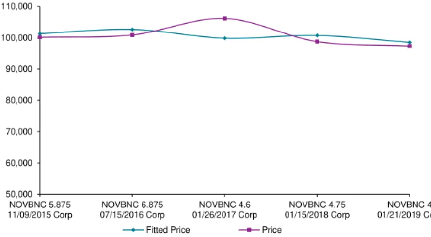
Figure 1: Model-implied price and actual price, August 4th(€)
Figure 2: Estimated long-term default probabilities (%)
With Vrgut’s model, it is also possible to observe the changes in the risk-neutral term structure of default probabilities, i.e., the way in which default probabilities vary with the time until the next promised cash flow. In general terms, a positive slope illustrates that the default probability increases for bonds with a closer cash flow date, whereas a negative slope shows that bonds with more time until the next promised cash flow date have a higher probability of default than those with less time until the next payment. In line with Vrgut’s findings, the shape of the term structure of default probabilities for BES’ bonds changes with
0.00% 2.00% 4.00% 6.00% 8.00% 10.00% 12.00% 14.00% 16.00% 18.00% 20.00% 0 1 -0 7 -2 0 1 4 0 3 -0 7 -2 0 1 4 0 5 -0 7 -2 0 1 4 0 7 -0 7 -2 0 1 4 0 9 -0 7 -2 0 1 4 1 1 -0 7 -2 0 1 4 1 3 -0 7 -2 0 1 4 1 5 -0 7 -2 0 1 4 1 7 -0 7 -2 0 1 4 1 9 -0 7 -2 0 1 4 2 1 -0 7 -2 0 1 4 2 3 -0 7 -2 0 1 4 2 5 -0 7 -2 0 1 4 2 7 -0 7 -2 0 1 4 2 9 -0 7 -2 0 1 4 3 1 -0 7 -2 0 1 4 0 2 -0 8 -2 0 1 4 0 4 -0 8 -2 0 1 4 0 6 -0 8 -2 0 1 4 0 8 -0 8 -2 0 1 4 1 0 -0 8 -2 0 1 4 1 2 -0 8 -2 0 1 4 1 4 -0 8 -2 0 1 4 1 6 -0 8 -2 0 1 4 1 8 -0 8 -2 0 1 4 2 0 -0 8 -2 0 1 4 2 2 -0 8 -2 0 1 4 2 4 -0 8 -2 0 1 4 2 6 -0 8 -2 0 1 4 2 8 -0 8 -2 0 1 4
July 15th
Investors react to a
series of negative
events
July 31th
Announcement of 3,600M€ losses
August 4th
Day after announcement
of recapitalization plan
19
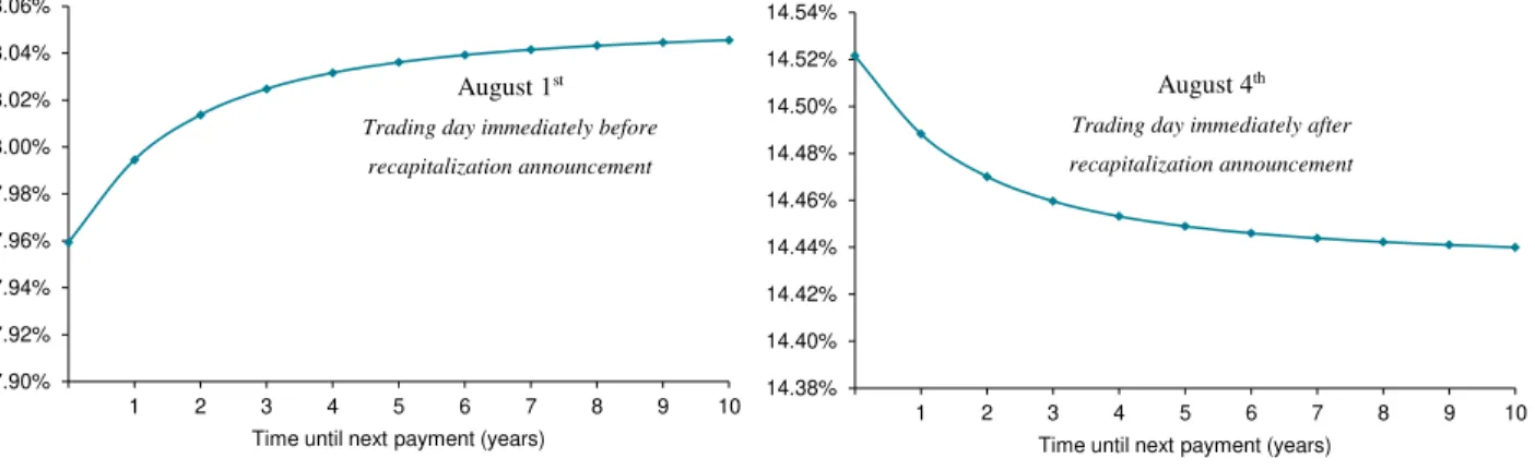
the announcement of the recapitalisation plan, going from a negative slope on August 1st (the
trading day immediately before the announcement) to a positive slope on August 4th. The slope remained positive for the remainder of the sample period.
Figure 3: Estimated risk-neutral term structure of default probabilities (%)
Throughout the selected period, the impacts of the abovementioned events did not affect implicit recovery values to the same extent as in default probabilities. After some fluctuations in the beginning of July, recovery value for BES stabilised around 70 cents on the euro.
In the CDS market, however, the reaction to these events is similar to the behaviour observed in implied default probabilities.
17.90% 17.92% 17.94% 17.96% 17.98% 18.00% 18.02% 18.04% 18.06%
1 2 3 4 5 6 7 8 9 10 Time until next payment (years)
August 1st
Trading day immediately before
recapitalization announcement
14.38% 14.40% 14.42% 14.44% 14.46% 14.48% 14.50% 14.52% 14.54%
1 2 3 4 5 6 7 8 9 10 Time until next payment (years)
August 4th
Trading day immediately after
20
Figure 4: 1-year CDS spread (basis points)
There is a noticeable increase in CDS spreads on July 31st, the day immediately after the losses were made public, thus reflecting investors’ lack of confidence in the bank’s creditworthiness. As with default probabilities, the maximum values for these spreads are recorded on August 1st. Moreover, there is an immediate reaction to the recapitalisation plan, as evidenced by the significant decrease (3.6 percentage points, on average) in spreads across all CDS maturities on August 4th. This decrease suggests that investors regained some trust on BES’ ability to cover its obligations, thus the demanded compensation for a protection buyer/seller is smaller, as a result of a decrease of the perceived default probability. CDS spreads keep decreasing until the end of the sample period, reflecting the market’s continued belief on the success of the recapitalisation/restructuring plan.
Comparing implied bond spreads with the prevailing CDS spreads on the market during the sample period allows for an assessment of market-implied perceptions of credit risk for the same entity by two different methods. Whereas CDS spreads directly represent investors’ perception of a certain entity’s credit risk, bond spreads represent the theoretical risk
premium required for corporate bonds in comparison to a risk-free instrument. By using
21
model-implied bond prices, the calculated bond spreads should incorporate the estimated default probabilities and recovery values, and as such allow for comparisons between model-implied and market credit metrics to be performed.
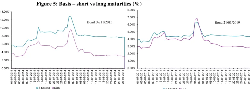
As detailed in equation (10), the basis results from the difference between CDS and bond spreads for the same maturity. Throughout the considered period, the basis is predominately negative across all selected BES’ bonds, meaning that CDS spreads were consistently above bond spreads. Therefore, investors were demanding a higher compensation on the CDS market than in the bond market, i.e., bonds were cheaper than entering into a CDS agreement at that time. Since both metrics echo the market’s perception of risk for BES, a negative basis suggests that bond-implied default probabilities were below the ones perceived on the CDS market.
Based on the belief that the two spreads should be co-integrated, an arbitrage opportunity could be considered to exist in this scenario. Assuming that, in equilibrium, the basis should tend to zero, a negative basis could be exploited by simultaneously taking a long position both on the bond and on the CDS markets, that is, buy the cheap instrument (bond) and sell the expensive one (sell credit risk, i.e., buy protection).
22
attributed to a similar adjustment for risk on both markets, i.e. perceived risk for BES was similar in both markets.
Figure 5: Basis – short vs long maturities (%)
Table 1: Summary of bases results for BES2
It should be noted that the existence of pure arbitrage opportunities is not common, and investors should approach these apparent opportunities with a certain level of precaution. The credit market is exposed to an array of uncontrollable and unpredictable factors, in addition to considerable transaction costs (bid-ask spreads), which have been found to have a sizeable impact on the potential gains of an arbitrageur.
2Bonds for BES have “NOVBNC” denomination, since at the time the data retrieved, these assets had already been
transferred to Novo Banco.
0.00% 2.00% 4.00% 6.00% 8.00% 10.00% 12.00% 14.00% 0 1 -0 7 -2 0 1 4 0 3 -0 7 -2 0 1 4 0 5 -0 7 -2 0 1 4 0 7 -0 7 -2 0 1 4 0 9 -0 7 -2 0 1 4 1 1 -0 7 -2 0 1 4 1 3 -0 7 -2 0 1 4 1 5 -0 7 -2 0 1 4 1 7 -0 7 -2 0 1 4 1 9 -0 7 -2 0 1 4 2 1 -0 7 -2 0 1 4 2 3 -0 7 -2 0 1 4 2 5 -0 7 -2 0 1 4 2 7 -0 7 -2 0 1 4 2 9 -0 7 -2 0 1 4 3 1 -0 7 -2 0 1 4 0 2 -0 8 -2 0 1 4 0 4 -0 8 -2 0 1 4 0 6 -0 8 -2 0 1 4 0 8 -0 8 -2 0 1 4 1 0 -0 8 -2 0 1 4 1 2 -0 8 -2 0 1 4 1 4 -0 8 -2 0 1 4 1 6 -0 8 -2 0 1 4 1 8 -0 8 -2 0 1 4 2 0 -0 8 -2 0 1 4 2 2 -0 8 -2 0 1 4 2 4 -0 8 -2 0 1 4 2 6 -0 8 -2 0 1 4 2 8 -0 8 -2 0 1 4 Z-Spread CDS Bond 09/11/2015 0.00% 1.00% 2.00% 3.00% 4.00% 5.00% 6.00% 7.00% 8.00% 0 1 -0 7 -2 0 1 4 0 3 -0 7 -2 0 1 4 0 5 -0 7 -2 0 1 4 0 7 -0 7 -2 0 1 4 0 9 -0 7 -2 0 1 4 1 1 -0 7 -2 0 1 4 1 3 -0 7 -2 0 1 4 1 5 -0 7 -2 0 1 4 1 7 -0 7 -2 0 1 4 1 9 -0 7 -2 0 1 4 2 1 -0 7 -2 0 1 4 2 3 -0 7 -2 0 1 4 2 5 -0 7 -2 0 1 4 2 7 -0 7 -2 0 1 4 2 9 -0 7 -2 0 1 4 3 1 -0 7 -2 0 1 4 0 2 -0 8 -2 0 1 4 0 4 -0 8 -2 0 1 4 0 6 -0 8 -2 0 1 4 0 8 -0 8 -2 0 1 4 1 0 -0 8 -2 0 1 4 1 2 -0 8 -2 0 1 4 1 4 -0 8 -2 0 1 4 1 6 -0 8 -2 0 1 4 1 8 -0 8 -2 0 1 4 2 0 -0 8 -2 0 1 4 2 2 -0 8 -2 0 1 4 2 4 -0 8 -2 0 1 4 2 6 -0 8 -2 0 1 4 2 8 -0 8 -2 0 1 4 Z-Spread CDS Bond 21/01/2019
Average Min. Max.
NOVBNC 5.875 09/11/2015 Corp -3.54% -4.81% -1.16%
NOVBNC 6.875 15/07/2016 Corp -2.18% -5.40% 0.86%
NOVBNC 4.600 26/01/2017 Corp -1.41% -2.41% 0.18%
NOVBNC 4.750 15/01/2018 Corp -1.21% -2.04% 0.12%
NOVBNC 4.000 21/01/2019 Corp -0.81% -1.56% 0.53%
23
Extending the analysis to the rest of the sample, it can be observed that the behaviour of market-implied default probabilities and recovery values varies across banks, time periods and countries.
24
Figure 5: Summary of bases results
Average Min. Max.
M illenium BCP
BCPPL 3.750 08/10/2016 Corp 2.02% -3.49% 5.70%
BCPPL 4.750 22/06/2017 Corp 3.63% -1.60% 5.82%
BCPPL 13.000 13/10/2021 Corp -0.71% -5.15% 1.46%
Caixa Geral de Depósitos
CXGD 3.384 15/12/2014 Corp -3.85% -8.14% -2.34%
CXGD 4.500 19/01/2016 Corp -1.78% -5.07% -0.51%
CXGD 4.455 20/08/2017 Corp -0.30% -3.43% 0.96%
CXGD 4.400 08/10/2019 Corp 1.09% -1.16% 2.33%
CXGD 5.320 05/08/2021 Corp -0.95% -2.68% 0.01%
Bankia
BKIASM 3.500 13/11/2014 Corp 4.31% 2.78% 6.06%
BKIASM 3.500 14/12/2015 Corp 3.44% -0.13% 5.45%
BKIASM 5.750 29/06/2016 Corp 2.98% 1.72% 4.45%
BKIASM 4.375 14/02/2017 Corp 3.93% 2.23% 5.73%
BKIASM 4.250 25/05/2018 Corp 2.98% 1.80% 4.51%
BKIASM 5.000 28/06/2019 Corp 2.80% 1.52% 4.41%
BKIASM 4.500 26/04/2022 Corp 2.33% 1.19% 3.85%
Novagalicia Banco
NOVAGA 3.125 15/04/2015 Corp -0.38% -1.70% 0.54%
NOVAGA 4.375 23/01/2019 Corp 1.05% -0.21% 1.82%
NOVAGA 4.900 31/07/2020 Corp 1.17% 0.09% 1.92%
Basis Bond
Average Min. Max.
SNS Reaal
SNSSNS 3.500 20/10/2015 Corp -0.55% -2.43% 0.56%
SNSSNS 4.250 26/09/2016 Corp -0.35% -2.10% 0.73%
SNSSNS 4.515 13/02/2017 Corp -0.67% -2.79% 1.17%
SNSSNS 5.360 18/09/2018 Corp 0.00% -1.54% 1.05%
SNSSNS 5.000 15/03/2019 Corp -0.61% -1.95% -0.08%
SNSSNS 3.500 28/08/2020 Corp 4.20% 3.70% 4.73%
Banco Espírito Santo
NOVBNC 5.875 09/11/2015 Corp -3.54% -4.81% -1.16%
NOVBNC 6.875 15/07/2016 Corp -2.18% -5.40% 0.86%
NOVBNC 4.600 26/01/2017 Corp -1.41% -2.41% 0.18%
NOVBNC 4.750 15/01/2018 Corp -1.21% -2.04% 0.12%
NOVBNC 4.000 21/01/2019 Corp -0.81% -1.56% 0.53%
Banca M onte dei Paschi di Siena
MONTE 3.750 02/01/2016 Corp -13.53% -27.64% -8.29%
MONTE 2.500 03/02/2017 Corp -4.26% -7.31% -3.04%
MONTE 5.000 09/02/2018 Corp -2.49% -4.26% -1.75%
MONTE 3.000 03/02/2019 Corp -1.66% -3.08% -1.08%
MONTE 5.000 21/04/2020 Corp 0.01% -0.78% 0.49%
MONTE 4.100 03/03/2021 Corp -0.19% -1.18% 0.29%
25
IV. Conclusion
This study attempts to identify basis-trading opportunities in the European banking sector over a period of 3 years, by comparing two different measures for the market’s
assessment of risk: market-observed CDS spreads and model-implied Z-spreads (following Vrgut’s framework, 2010). Assuming non-arbitrage pricing, these two metrics should convey the same information for a given financial instrument, i.e., the CDS-bond basis should be zero.
Considering a sample of 10 banks, this analysis was performed on periods of a “default”
event, such as restructuring programs, government-sponsored bank bailouts and/or recapitalisations. Overall, it can be concluded that, while implied default probabilities and recovery values greatly depend on the reference entity, geography and time, the majority of bases were, on average, negative. Additionally, across the selected sample, the basis is larger for bonds with smaller maturities. This suggests that there were arbitrage opportunities throughout the sample periods, potentially more profitable for smaller maturity bonds. As such, the arbitrageur should buy the bond, while simultaneously buying the CDS instrument (selling protection), capitalizing these opportunities as the basis approaches its long-term equilibrium.
26
artificially larger bases. In addition, given the simplicity of the calculations employed for the bond spread, the estimated basis may not be the most accurate proxy for assessing basis-trading opportunities.
27
V. Appendix
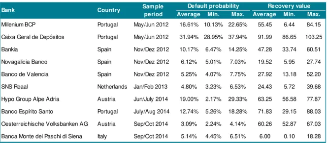
Table 2: Estimated parameters –Vrgut’s model
Average Min. Max. Average Min. Max.
Millenium BCP Portugal May/Jun 2012 16.61% 10.13% 22.65% 55.45 6.44 84.15
Caixa Geral de Depósitos Portugal May/Jun 2012 31.94% 28.95% 37.94% 91.99 86.65 103.25
Bankia Spain Nov/Dez 2012 10.17% 6.47% 14.25% 47.28 33.74 60.51
Novagalicia Banco Spain Nov/Dez 2012 6.12% 5.01% 7.03% 19.52 5.95 27.74
Banco de Valencia Spain Nov/Dez 2012 5.25% 4.07% 7.75% 27.92 13.18 52.20
SNS Reaal Netherlands Jan/Feb 2013 4.80% 3.23% 6.53% 24.43 5.72 39.68
Hypo Group Alpe Adria Austria Jun/July 2014 19.00% 2.17% 29.33% 63.25 56.58 77.87
Banco Espírito Santo Portugal July/Aug 2014 12.74% 5.26% 18.28% 71.83 29.15 88.03
Oesterreichische Volksbanken AG Austria Sep/Oct 2014 3.09% 2.24% 4.14% 60.26 52.87 67.03
Banca Monte dei Paschi di Siena Italy Sep/Oct 2014 5.14% 4.45% 6.51% 6.00 0.10 18.28
Bank Sam ple
period
Default probability Recovery value
28
References
Alexopoulou, Ioana, Magnus Andersson, and Oana Maria Georgescu. 2009. “An Empirical Study on
the Decoupling Movements between Corporate Bond and CDS Spreads”. ECB Working Paper No.
1085.
Bai, Jennie, and Pierre Collin-Dufresne. 2013. “The CDS-Bond Basis”. Journal of Economic
Literature.
Blanco, Robert, Simon Brennan, and Ian Marsh. 2005. “An Empirical Analysis of the Dynamic
Relationship between Investment Grade Bonds and Credit Default Swaps”. Journal of Finance, 60,
2255-2281.
Coleman, Thomas S.. 2008. “A Primer on Credit Default Swaps (CDS)”. Working paper:
http://papers.ssrn.com/sol3/papers.cfm?abstract_id=1555118.
De Wit, Jan. 2006. “Exploring the CDS-Bond Basis”. National Bank of Belgium Working Paper No.
104.
Fagan, Gabriel and Vitor Gaspar. 2007. “Adjusting to the Euro”. ECB Working Paper No. 716.
Gourinchas, Pierre-Olivier, and Maurice Obstfeld. 2012. “Stories of the Twentieth Century for the
Twenty-First”. American Economic Journal: Macroeconomics 4(1): 226–65.
Hull, John, Mirela Predescu and Alan White. 2004. "The Relationship between Credit Default Swap
Spreads, Bond Yields, and Credit Rating Announcements". University of Toronto Working Paper.
Jarrow, Robert, David Lando and Stuart M. Turnbull. 1997. “A Markov Model for the Term Structure
29
Laeven, L. and Fabián Valencia. 2012. “Systematic Banking Crises Database: An Update”. IMF
Working Paper No. 12/163.
Lane, Philip R. 2012. “The European Sovereign Debt Crisis.” Journal of Economic Perspectives
26(3): 49–68.
Lane, Philip R., and Gian Maria Milesi-Ferretti. 2011. “The Cross-Country Incidence of the Global
Crisis.” IMF Economic Review 39(1): 77–110.
Li, Haitao, Weina Zhang and Gi Hyun Kim. 2011. “The CDS-Bond Basis Arbitrage and the Cross
Section of Corporate Bond Returns”. Working Paper, National University of Singapore.
Merton, Robert C. 1974. “On the Pricing of Corporate Debt: The Risk Structure of Interest Rates”.
Journal of Finance 29: 449-470.
Schoenmaker, D. and Toon Peek. 2014. “The State of the Banking Sector in Europe”. OECD
Economics Department Working Papers No. 1102.
Svensson, Lars E. O., 1994. “Estimating and Interpreting Forward Interest Rates: Sweden 1992 –
1994”. NBER working paper No. 4871.
Vrgut, Evert B. 2010. “Estimating Implied Default Probabilities and Recovery Values”. Journal of