INSTITUTO SUPERIOR DE ECONOMIA E GESTÃO

(1)

UNIVERSIDADE TÉCNICA DE LISBOA

INSTITUTO SUPERIOR DE ECONOMIA E GESTÃO

MESTRADO EM: Economia Monetária e Financeira

TERM STRUCTURE OF CREDIT SPREADS WITH AFFINE

PROCESSES

DMITRY SHIBAEV

Orientação: Prof. Jorge Barros Luís

Júri:

Presidente:

Profª. Maria Rosa Borges

Vogais:

Prof. Elísio Brandão

Prof. Jorge Barros Luís

(2)

TERM STRUCTURE OF CREDIT SPREADS WITH AFFINE PROCESSES

Dmitry Shibaev

M.Sc.: Monetary and Financial Economics

Supervisor: Prof. Jorge Barros Luís

Concluded in:

ABSTRACT

A brief review and a comparison between Structural and Intensity mode is

presented in the first section with an argument in favor of Intensity models

based on the quality of information available to market participants.

Next, an Intensity model with an affine (constant plus linear) parametrization of

the intensity parameter driven a by a set of latent variables is formulated for the

Euro Credit Default Swap (CDS) curve. Latent variables in the intensity

parameter are assumed to follow uncorrelated CIR processes. Furthermore the

model parameters, the latent variable processes and implicit risk-neutral default

probabilities are estimated with an application of a Linearized Kalman Filter

approach and a Likelihood maximization algorithm.

A conclusion is reached that a model with two latent variables is able to account

for 95%, 89%, 98% and 99% of the variations in 3, 5, 7 and 10-year maturities

of the CDS curve.

Keywords: credit risk, affine, intensity models, CIR, term-structure, kalman filter.

(3)

ESTRUTURA TEMPORAL DE SPREADS DE CRÉDITO COM PROCESSOS

AFFINE

Dmitry Shibaev

Mestrado em: Economia Monetária e Financeira

Orientador: Prof. Jorge Barros Luís

Provas Concluidas em:

RESUMO

Um breve resumo e uma comparação entre os modelo Estruturais e modelos

de forma Intensiva é apresentado na primeira secção do trabalho, com um

argumento a favor dos modelos de forma Intensiva baseado na qualidade de

informação disponível aos participantes do mercado.

De seguida, é formulado um modelo de forma Intensiva para a a curva “Credit

Default Swap (CDS)” da zona Euro com a parametrização “affine” (constante

mais linear) do parâmetro de intensidade que por sua vez é movido por um

conjunto de variáveis latentes. É assumido que as variáveis latentes seguem

processos CIR não correlacionados. Os parâmetros do modelo, processos das

variáveis latentes e probabilidade de incumprimentos risco-neutrais implícitas

são estimados com a aplicação da versão Linearizada do Filtro Kalman em

conjunto com o algoritmo de Maxima Verosimilhança.

Por fim conclui-se que o modelo com duas variáveis latentes é capaz de

explicar 95%, 89%, 98% e 99% das variações nas maturidades de 3,5, 7 e 10

anos da curva CDS.

Palavras Chave: risco de crédito, affine, modelos de forma intensiva, CIR,

estrutura temporal, filtro kalman.

(4)

AGRADECIMENTOS

Em primeiro lugar queria agradecer a minha família por me ter apoiado e

motivado desde o início. Também gostaria agradecer o Prof. Jorge Barros Luís

pelo tempo dispensado na orientação deste trabalho e pela forma práctica

como conduziu as reuniões. Agradeço o Prof. Paulo Brito e Prof. Pedro Júdice

pelos comentários e sugestões. Agradeço o Rui Cabral, Ricardo Santos, José

Cerveira e Nuno Palma pelas discussões continuas.

(5)

3 List of Figures

Figure 1 - Two CDS curve examples……….. 9

Figure 2 - CDS series and the Normal Distribution………... 10

Figure 3 - One-factor observed and estimated CDS premia………... 18

Figure 4 - Estimated process for the latent variable X_₁……… 20

Figure 5 - Comparison of the estimated latent variable process with the four CDS premia….. 21

Figure 6 - Two-factor observed and estimated CDS premia……….. 22

Figure 7 - Estimated processes for the latent variables X₁ and X₂……… 23

Figure 8 - Relative fit of the one-factor and the two-factor model……….. 24

Figure 9 – Principal Components………. 31

List of Tables

Table 1 - Descriptive Statistics of CDS premia in Differences………... 9

Table 2 - Parameter estimates for one-factor model………... 19

Table 3 - Parameter estimates for two-factor model……… 20

Table 4 - Model implied risk-neutral probabilities of default………... 24

(8)

1 Introduction

The purpose of this paper is to study the forces responsible for movements in credit spreads at

di¤erent maturities. A credit spread is usually perceived as the premium demanded by the investors

to hold risky (subject to default) assets over risk-free counterparts. Examples of these assets are

corporate bonds that have credit risk embedded due to the possibility of a company’s default. On

the other hand examples of risk-free assets are bonds issued by governments of developed countries

carrying zero1 _{credit risk due to the general belief that it is impossible for example the United}

States government to default on its obligations. A common misleading interpretation emerges:

The di¤erence in return between risky and risk-free bonds is the credit spread. This interpretation

is incorrect because there are two additional components in this di¤erence besides credit spread:

liquidity premium and tax premium. The presence of these two components imply that bonds are

not an ideal choice for the study of credit spreads.

Alternative …nancial instruments are available on the markets that bear a better re‡ection of

credit spreads. One that focuses directly on credit risk and establishes a price for it in a market

environment is a Credit Default Swap (CDS) contract. CDS contracts are credit derivatives with

a standardized speci…cation dictated by the ISDA2 and are comprised of three main components:

a risky underlying asset; the contracting party normally holding this asset and an insuring party.

The risky asset is usually a senior, unsecured bond emitted by a corporation subject to default

risk. The contracting party holding this asset enters into such a contract with the view to o¤set

the potential default risk of the corporation in return for a semiannual premium payment to the

insuring party. Thus a CDS contract takes the form of a standard insurance policy where the

insured capital is the risky asset and where the premium prices directly re‡ects the risk involved.

CDS contracts apart from having an appealing de…nition for the credit risk subject, also bene…t

from being traded on organized Over the Counter Markets with …xed maturities from 1 to 10 years.

Availability of a multidimensional dataset lets one study the time-series and cross-section properties

of the variable. Models that take into consideration these two dimensions are commonly referred

to asterm structure models.

The paper proceeds as follows: In section 2 structural and intensity credit models are compared.

Section 3 provides a description of the CDS timeseries properties and in section 4 a formulation of

an intensity model is presented. In section 5 the model estimation methodology is discussed and

in section 6 results are presented. I conclude with section 7.

1_{For the sace of this dicussion I assume that government bonds are risk-free. Government bonds of developed}

countries with a solid politic system, stable economy and sound …nancial markets are usually attributed a AAA rating by the rating agencies which is although not risk-free, but very close to.

(9)

2 Credit Models

In the theory of credit risk one is generally limited to a choice between two di¤erent modeling

approaches: The classicStructuralmodels, or the more recentIntensitymodels. These are generally

perceived as rivals, until the recent publication of two papers by Du¢e & Lando (2001) and Çetin

et al. (2004) demonstrating that the two models, although based on distinct assumptions are

actually of the same kind if an additional relatively weak assumption is added to both of them.

This vital assumption linking both models into one is that the market participants are less informed

than the managers. A distinction between information sets implies di¤erence in perception of a

company’s health by two sets of agents, the ones participating in the market and the ones controlling

the company.

In order to get a better grasp of the two modeling approaches, in the next two subsections I

will brie‡y review both of them and provide an intuition on under what circumstances one should

be chosen over the other.

2.1 Structural Credit Models

Since the early 70’s with the publication of two in‡uential papers on pricing of defaultable

con-tingent claims by Merton (1974) and Black & Cox (1976), their ideas became standard for credit

risk modelling. Almost exclusively all subsequent thirty years of research were based on their

fundamental idea that a …rm’s value could be modelled as a standard, continuous di¤usion process

with default occurring when a …rm’s value drops to a level where repayment of outstanding debt

can not longer be warranted. A number of commercial packages, allegedly predicting the risk of a

…rm’s default have been developed, such as Moody’s KMV or JPMorgan - CreditGrades3. The

termStructuralis at times used to classify these models, as explicitly de…ning the structure of how

a …rm’s value evolves throughout time.

Consider a …rm’s value to be well represented by a di¤usion process where is the …rm’s asset

rate of return, asset volatility andWta standard Brownian motion

dVt= Vtdt+ VtdWt (1)

This equation intuitively tells us that a …rm’s value is expected to ‡uctuate randomly around its

long-term growth path de…ned by the variable . Fluctuations are not deterministic and thus do

not permit to infer exactly on where a …rm’s value will be at any period in time, but it provides

3_{Documentation on Moody’s KMV and CreditGrades models can be found by the following to links respectively:}

(10)

enough information to construct a probability distribution on the likelihood of being above, or

below a certain level at any future date.

Lets now consider that for a …rm to stay alive its asset value must at all times remain above

a certain barrier K. This assumption is quite reasonable as many …rms in the market carry

a signi…cant amount of debt, and if their asset value drops below the value of debt, the …rm

technically goes into default. Many times it is convenient to have an estimate of the probability

that a …rm will not default before some time , as in the case when a decision is made on whether

to lend funds to a …rm and under what conditions.

Formally the probability of survival Qin structural models depends on a …rm’s internal

para-meters , , current asset valueV0 and the default barrierK, as

Q( > T) =f(V0; K; ; ; T) (2)

where the implicit function f( ) can vary according to the de…nition of randomness in the asset process. IfdW is assumed to follow a normal distribution, as is usually done, then functionf( )

will be something similar to the well-known Black-Scholes equation.

2.2 Intensity Credit Models

Intensity models were …rst introduced by Jarrow & Turnbull (1995), Jarrow et al. (1997) and

extended in papers such as Du¢eet al. (1996), Lando (1998), Du¢e & Singleton (1999), Du¤ee

(1999). These models bear signi…cant di¤erences to structural models. As opposed to structural

models, intensity models are silent about why default occurs. They do not make assumptions

on the evolution of …rm’s asset value. Moreover, capital structure, volatility, leverage ratio and

expected return play no direct role in the de…nition of the survival probability. In intensity models

survival probability is calculated on the basis of a binary outcome of a point process. A …rm

defaults if the underlying process assumes a value of 1, implying that the probability of surviving

is equivalent to the probability of a point process not jumping from 0 to 1.

The term intensity comes from the de…nition of the underlying point processes. A Poisson

process is one example where the intensity is the only variable controlling the probability of a

jump. In fact Poisson processes have much in common with the general speci…cation of intensity

models. Consider a standard Poisson process4 _{with a known intensity, the probability that the}

4_{From statistics, a homogeneous (time independent) Poisson process, with terminology adapted to credit risk,}

states that the probability ofn_{defaults within a …xed time interval is controlled by an intensity} _{through the}

relation

P(n=k) =e k

(11)

process will not jump during a certain time interval depends only on the intensity for the same

time interval through the relation

P(n= 0) =e (3)

Extending this logic to the construction of intensity models, we can de…ne the probability of

survival past timeT as

Q( > T) =e (4)

This last equation is the main building block for intensity models, extremely simplistic in

its construction, but su¢ciently versatile to accommodate a vast variety of parametrization. In

fact, as we will see later, the intensity parameter is not required to remain constant, or to

be deterministic. The intensity variable can be allowed to take on alternative functional forms,

be a¤ected by external macroeconomic and internal, …rm speci…c variables of deterministic or

stochastic nature.

2.3 Equivalence between Intensity and Structural Models

As in Jarrow & Protter (2004). Structural models assume complete knowledge of a very detailed

information set (up to the stochastic process of the asset price). This information is normally

thought to be available to managers. With an extremely re…ned information set, up to the point

of knowing the value of assets at each point in time implies that a …rm’s default is predictable, but

this is not necessary the case. In contrast, intensity models assume knowledge of a less detailed

information set (up to the knowledge of the default probability). This information set is normally

though to be available to the market.

Du¢e & Lando (2001) and Çetinet al. (2004) demonstrate that structural and intensity models

are equivalent by assuming that the asset di¤usion process in the structural models is not perfectly

observable. An interpretation is that accounting reports and press releases either purposefully or

inadequately add extra noise that obscures the market’s knowledge of the …rm’s asset value.

Both papers reach the same, crucial conclusion that brought intensity models greater attention

and acceptance from academics and practitioners:If the asset value is not perfectly observable then

the structural models are just a special case of more general intensity models. Intuitively, if the

asset value is not perfectly observable then the market has no way of knowing the exact function

in equation 1 and mathematically by adding noise to this function makes it reducible to the one

(12)

When choosing a model one must take into consideration two main factors: the model’s ability

to mirror empiric stylized facts and to admit a viable speci…cation for econometric estimation.

More ‡exible intensity models are able to better adhere to these two requisitions and in addition,

as argued above, have the advantage of nesting a structural model within. Since the publication of

seminal papers on intensity models, they have been slowly becoming the models of choice especially

in term-structure modeling problems. Recent examples of their applications to CDS premia are

those of Schneideret al. (2007) and Pan & Singleton (2007).

3 Data Description

According to Reyngoldet al. (2007), CDS prices are fairly pure indicators of credit risk because

their structure separates the credit risk component from other asset risks and premiums, such as:

Interest rate risk, currency risk and tax premium normally present in bonds. In addition they

are light instruments in the sense that one does not need to fund an entire bond position, for

example, to have essentially the identical credit risk exposure. Finally CDS pricing has become

liquid with standardised ISDA contracts and exponentially growing markets. Total market size of

CDS (notional outstanding) was 17 trillion USD by broker estimates in April 2006.

In the empirical application I will use a CDS iTraxx index of High Volatility European

compa-nies taken from Reuters Xtra 3000 and consider it as a good overall credit risk representation in the

euro area. This speci…c series was chosen due to its relatively extensive timeseries, greater number

of maturities if compared to other iTraxx series and more liquidity if compared to contracts on

individual counterparties. Daily iTraxx HiVol series for 3, 5, 7 and 10 year maturities, spanning

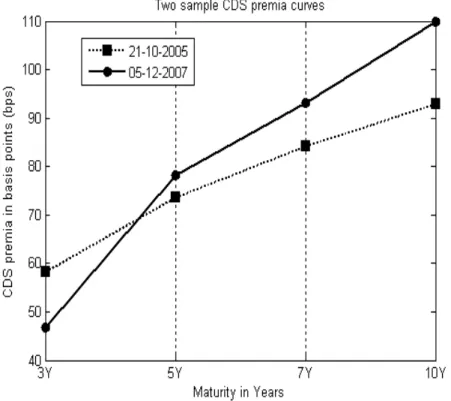
from 21-10-2005 to 5-12-2007, with a total of 537 data points were extracted. The series’

descrip-tive statistics are very similar to what is expected from any …nancial series: a skewed distribution

with a large kurtosis, indicating non-normality. Two sample CDS curves are presented in Figure

1.

3.1 Sample Distribution Statistics

When looking at a time series distribution it is usually su¢cient to analyse the …rst four moments to

get a picture of its characteristics: mean, variance, skewness and kurtosis. These are calculated for

(13)

Figure 1: Two CDS curve examples, one from the beginning and the other from the end of the sample. On the vertical axes the CDS premia is quoted in basis points (1 bps = 0.01%).

and presented in a table below for the available range of maturities

Table 1: Descriptive Statistics of CDS premia in Di¤erences5

3Y 5Y 7Y 10Y

Standard Deviation 0.00015 0.00021 0.00022 0.00021

Skewness 0.2647 -0.1278 -0.7206 -0.4733

Kurtosis 10.5127 13.8708 16.7872 15.3054

A …rst observation can be made, shorter maturity contracts tend to exhibit higher volatilities,

especially the 3 year contracts with more than 3 times the volatility of the 10 year contract. This

can be an indication that shorter maturity contracts respond more to short-term market turmoils

while the longer maturities are more a¤ected by long-term economic trends that tend to be less

volatile.

Skewness gives an indication on the sample distribution tilt, leftward (negative value) or

right-ward (positive value) and the size of this tilt. It is surprising to see that only the 3 year maturity

exhibits a positive skewness indicating mostly positive movements. The fourth moment, Kurtosis,

(14)

gives an indication on the concentration of values around the distribution mean, as well as the

tail size. A time-series with a tight concentration of data points around the distribution mean,

and a signi…cant number of outliers is bound to exhibit a large kurtosis. CDS time-series is no

exception with kurtosis above 10 across all maturities (in comparison to a kurtosis of 3 in a normal

distribution).

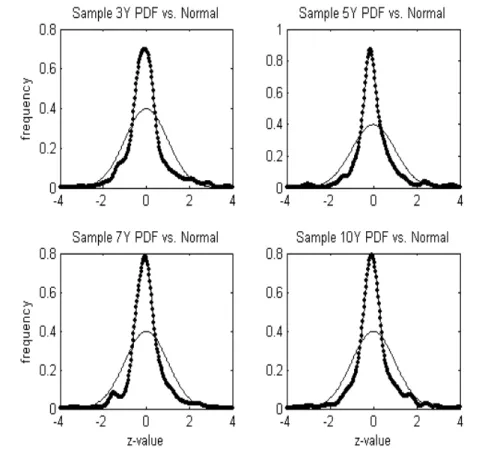
Figure 2 visually con…rms the analysed descriptive statistics and motivates the argument against

a single, Gaussian model to capture the full distribution spectrum of CDS premia, such as a

structural model.

Figure 2: Comparison between the diferenciated CDS premia series and the normal distribution.

4 Intensity Model for CDS Premia

CDS contracts are credit derivatives that give the buyer protection against default of the underlying

asset and issuer, the exposure to this credit risk. Individual CDS contracts on an underlying asset

are constructed in such a form that in case of a default, the selling party is obliged to reimburse the

buying party the full covered notional amount. In return, up to the date of the default the buying

(15)

similar way to a common insurance policy. In a complete market where no arbitrage opportunities

may exist, equilibrium is attained when the expected sum of all the premium payments are equal

to expected pay-out in case of a default.

I will denote A0 as the expected sum of quarterly premiums payments by the buying party

over the life of the contract. Where c is the constant premium, T the term of the contract, r

the risk free interest rate6 _and ₁

>T an indicator function taking on value 1 if no default occurs prior to T and 0 otherwise. Under the risk neutral measureQ, the expected current value of all

the premiums is a relation between the risk free interest rate and the indicator function implying

premium payments up to the date of the default

A0=EQ

2

4c

4T

X

j=1

e r(j4)1 >j4

3

5 (5)

In the world where interest rates are deterministic one can work through the expectation and

arrive at a probability for the indicator function, being the only unknown parameter. The equation

above can thus be simpli…ed to take on a more convenient form

A0=c 4T

X

j=1

e r(4j)_Q > j

4 (6)

where as has been seen before,Q > j₄ is the probability of survival past ₄j corresponding to the periodic premium payment date.

Further I will denoteB0 as the expected present value of the pay-out in the case of a default,

with all other parameters as before

B0=EQ e rT[1 1 >T] (7)

It is trivial to see that if1 >T indicates survival past timeT, then1 1 >T indicates the contrary, default prior to timeT. Working through the expectation, and as before with deterministic interest

rates, the above equation simpli…es to

B0=e rT[1 Q( > T)] (8)

Furthermore, in an arbitrage free market, the equality relation betweenA0 andB0 must hold.

By equaling the two and solving for the premium parameter I arrive at an equation relating the

6_{For the interest rate I will use the German zero-coupon Bunds at available maturities and …ll missing data}

(16)

CDS premia to the probabilities of survival

c= e

rT_[1 _Q₍ _{> T}_)]

P4T j=1e

r₍j

4)_Q _>j 4

(9)

From here onward one can either estimate the premium market price if the survival probabilities

are known, or estimate the probabilities of survival if market premiums are known. Information

regarding probabilities of survival are regularly published by rating agencies, thus letting one

estimate CDS premia by a simple application of the above equation. The objective of this paper is

however, related to the latter problem, estimating not only the probabilities of survival, but also

extracting the forces that move them.

4.1 Intensity Representation of the Survival Probability

The next question is how to give some explicit form to the probability of survival. As it has

been seen in the introductory section, intensity models are built on point processes where the

probability of survival is de…ned as the probability of no jumps in the point process within a

certain time interval. The probability of survival past timeT is given by equation 4 which could

be back substituted into equation 9 to get rid of the probability parameter, but this would still leave

the model depending on the intensity variable, , with up to now unknown form. The intensity

variable could be left constant and estimate likewise, however signi…cantly constraining the model

dynamics. An alternative approach is to let the intensity take on a stochastic form, by which

adding richer dynamics to the model and letting the probability of survival vary through time.

4.2 Stochastic A¢ne Intensity

A¢ne intensity as will be described here and a¢ne models in general are characterized by all the

variables having a constant plus linear relation between themselves. What makes a¢ne models

more attractable when compared to other functional forms is their direct interpretation of

parame-ters and maybe most important of all, they generally admit closed form solutions. A¢ne models

were …rst introduced and popularized by Du¢e & Kan (1996) with the publication of a seminal

paper on interest rate yield-curve modeling. Their initial approach was later extended by Du¢e

et al. (2000) to show that every exponential a¢ne jump-di¤usion model admits a closed-form

so-lution and includes a wide array of yield-curve models as special cases, such as the Vasicek (1977)

and the Coxet al. (1985) model.

Returning to the survival probability, a stochastic version is attained when the intensity follows

(17)

intensity implies that the survival probability is no longer constant across its time horizon and

must be evaluated over the full trajectory of the intensity variable. In mathematical terms, a

stochastic survival probability past timeT is

Q( > T) =EQh_e R0T (s)ds

i

(10)

The probability is a¢ne in construction if the intensity parameter is a linear function of some

underlying latent variables (I will use the terms variables and factors interchangeably throughout

this paper). Latent variables, X, take their name from their unobservable nature, similar to

principal components in a principal component analysis and in general do not carry any obvious

economic interpretation7_{. Formally an a¢ne intensity takes the form}

(Xt) = 0+ 1Xt (11)

where there is no constrain on the number of latent variables entering the above equation. In a

univariate case Xt is a just a single variable, whereas in a multivariable case Xt and 1 can be

n-dimensional vectors.

However for a model to be classi…ed as a¢ne it is insu¢cient for the intensity to be a linear

function of latent variables, as the stochastic process governing each latent variable also has to be

of a¢ne form8_{. In an It¯o representation of the stochastic process for latent variables}_X

t

dXt= (Xt)dt+ (Xt)dWt (12)

where (Xt) and (Xt) are implicit vectors in Rn and Rn n controlling the deterministic and variable parts accordingly, and Wta standard Brownian motion. The model is a¢ne if both the deterministic and variable parts have a linear plus constant dependence on each other

(Xt) = 0+ 1Xt (13)

(Xt) =

p

0+ 1Xt

7_{In the …eld of interest rate term structure modeling, attempts have been made to label latent factors with}

intuitive names such aslevel, slope andcurvature. For further discussion consult Cristensenet al. (2007). 8_{For a technical reference on the necessary and su¢cient conditions of a¢ne models, as well as a mathematical}

(18)

4.3 CIR Process as a Special Case

A¢ne models are malleable enough in the de…nition of the latent variable di¤usion process to

encompass a wide variety of alternative speci…cations, only constrained by the technical conditions

as explained in Dai & Singleton (2000). One of these examples is the Coxet al. (1985) process,

widely referred to as the CIR process initially devised for the modeling of interest rates. A CIR

di¤usion process takes the form

dXt=k( Xt)dt+

p

XtdWt (14)

with constant parametersk, and . Parameter has the interpretation of the long-run mean,

k the speed of convergence to the long-run mean and volatility. This process is a¢ne, as its

parameters map directly to the ones in equation 13,k = 0,k= 1, = 21.

CIR and Gaussian processes are the best known examples of a¢ne di¤usions. The two classes

di¤er with respect to their assumptions about the variance parameter. Gaussian processes have

a constant variance while CIR processes introduce conditional heteroskedasticity by allowing the

variance to depend on the state variable which as noted by Bates (1996) and Heston (1993) is an

important ingredient to account for skewness and large kurtosis in …nancial timeseries, as the ones

presented in section 3.1.

4.4 Loss Given Default (LGD)

Central to the pricing of any insurance policy or a derivative on an asset subject to default is Loss

Given Default, or simply LGD. By omitting loss given default, one would tend to overprice the

premiums by implicitly assuming that the insurer is subject to bear the full loss of asset value

at default, which is not generally the case, as recoveries tend to vary anywhere from 20% in the

services sectors to 80% in capital intensive sectors9_.

There are two alternative ways to account for loss given default in the model. The simpler one,

which I will use in this paper, usually referred to asRecovery of Market Valueand the second one,

Recovery of Face Value. Based on a simulation study, Du¢e & Singleton (1999) provide an empiric

comparison between the two methods and their main …ndings suggest that distinction between the

two is negligible to a few basis points, thus supporting my choice of the simpler speci…cation.

In the Recovery of Market value10 _{formulation, loss given default parameter}_l_{enters the model}

9_{A study by Altman & Kishore (1996) illustrates that loss give default tends to vary signi…cantly between sectors}

and provides an estimate for this variable per industry sector on the basis of historic evidence.

1 0_{Note that Recovery refers to the fraction recovered in the case of a default, while Loss Given Default (LGD)}

refers to the fraction lost in the case of default. There should be no ambiguity between the two, as Recovery is1 l_,

(19)

through a multiplicative relation with the intensity and a¤ects only the pay-out part in the case

of a default (B0). In a stochastic a¢ne setting the expected pay-out at default with a non-zero

recovery now becomes

B0 = e rT

h

1 Q~( > T)i (15)

~

Q( > T) = EQhe R0Tl (s)ds

i

(16)

The intuition behind multiplying the intensity by the loss given default is as follows. Decreases

in the intensity translate into increases in the probability of survival which in turn translate into

decreases in the premium prices that the insurer is willing to accept under the view that not all

of the asset value will be lost in a case of a default. And asl is constrained in the domain[0;1], including it in the model e¤ectively increases the probability of survival by arti…cially lowering the

intensity parameter11.

4.5 Model Solution

Probably the greatest di¢culty in …nding a solution to a term structure model, as the one in

this paper, is getting rid of expectations and evaluating the integral in the exponential function.

Fortunately enough, we can make use of the Feynman-Kac approach by reducing the expectation

to a partial di¤erential equation that for an a¢ne con…guration always admits a solution of the

form Q( > T) =e (T)+ (T)X where (T) and (T) solve a partial di¤erential equation. The approach itself is outlined in Appendix 8.1

Explicitly assuming a CIR process for latent variables has a further advantage that the solution

has been demonstrated by Coxet al. (1985) and takes the form12

Q( > T) =EQh_e R0T (s)ds

i

= (T)e (T)X (17)

where (T)and (T)are known explicitly13

1 1_{A formal demonstration of how the Recovery of Market Value is introduced into a¢ne intensity models can be}

found in Du¢e (2005).

1 2_{Note that by assuming a CIR process for latent variables I inevitably simplify equation 11 by setting} ₀ _{= 0}

and 1= 1.

1 3_{While the presented solution is for a univariate case, extentions to include aditional latent variables}

(20)

(T) =

"

2 e(k+q+ )T2

( +k+q) (e T _{1) + 2}

#2k

2

(18)

(T) = 2 e

T ₁

( +k+q) (e T _{1) + 2} (19)

= (k+q)2+ 2 2

1 2

(20)

The parametersk, and are from the CIR di¤usion process in equation 14 and the variable

qis the market risk premium. Positive risk premiums arise forq <0.

5 Model Estimation

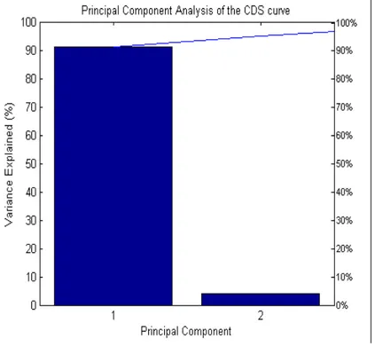
With the use of a principal component analysis I conclude that roughly 91% of the movements in

CDS premia across all four maturities can be explained by one latent variable and around 95%

by two (refer to Appendix 8.4 for details). Based on these statistical facts I estimate two sets of

models, the …rst one with a single latent variable, and another one with two latent variables.

For the estimation method, I use a discrete Kalman Filter approach. As discussed in Chen

& Scott (2003), from available alternatives, namely General Method of Moments (GMM) and

Simulated Maximum Likelihood (SML), Kalman Filter is usually the preferred choice, as it

gen-erally provides lower standard errors for parameter estimates than GMM and is signi…cantly less

time consuming than SML. The main disadvantage of the Kalman Filter approach is that it

im-plicitly assumes normality for the estimation error distribution, sometimes di¢cult to justify in

applications to …nancial time series14_.

Both one-factor and two-factor models share the same set of equations, only varying in the

number of parameters, thus without loss of generality I present the general model and then provide

estimate results for each one of them.

For the application of the Kalman Filter, the model and the processes governing the evolution

of latent variables need to be transformed into a compatible set of equations. The …rst equation is

usually referred to as themeasurement equation,linking latent variables to observable CDS premia,

and the second equation astransition equation,de…ning the value for latent variables at each point

in time. The measurement and transition equations to be used in estimation are presented below

1 4_{A brief review with additional references to alternative estimation methodologies, their advantages and}

(21)

respectively

c =

e rTh₁ _~(_T₎_e ~(T)Xi

P4T j=1e r(

j

4) (j 4)e (

j

4)X

+Rt (21)

Xt = 1 e k +e kXt 1+Ft (22)

The measurement equation is obtained by substituting the probability of default from equation

17 by the function for CDS premia in equation 9 and including an additional error term Rt to account for discrepancies between observed and model predicted values. At this point it is

convenient to note that a Kalman Filter is devised to only handle linear functional forms for

the measurement equation, while the one presented above is clearly a non-linear one. Slightly

di¤ering from the work of Du¤ee (1999), where the model was linearized around each observation,

I linearize the model only once at the beginning of estimation around the long-term mean of the

latent variable, thus gaining signi…cant improvement in the speed of estimation from roughly two

days to a few minutes15_.

The transition equation is a discrete solution to the continuous version of the CIR process in

equation 14. As in the continuous version, is the long-run mean,k is the speed of convergence

to the long-run mean andFt is the random part of the equation that assumes a somewhat more complicated form16_{. It has been noted by a number of authors including Cox}_{et al.} _{(1985), Du¤ee}

(1999), Chen & Scott (2003) and Duan & Simonato (1999) that a central problem in estimating

CIR processes is that non-negativity of its variance is at times di¢cult to assure due to the way

the latent variable a¤ects the variable partFtof the process. Negative values in the latent variable lead to negative volatilities. To remedy this problem, similarly to Du¤ee (1999) I will impose a

zero barrier for the latent variables. Alternative solutions for negative variance are discussed in

Appendix 8.3.1.

1 5_{Refer to Appendix 8.3 for a discussion on alternative linearization techniques.}

1 6_{As discussed in the original paper on CIR processes Cox} _{et al.} _{(1985), in a di¤usion process with square-root} volatility the transition distribution is a non central chi-squared, rather than normal as in a gaussian di¤usion process. This di¤erence in volatility slightly alters the usual representation of the variable term in the transition equation to

F_t₌ 2h_X

t 1 e k e 2k +₂ 1 e k 2

i

(22)

6 Estimation Results

6.1 One-Factor Intensity Model

The results in this section were generated by estimating the model in equation 21 with one

la-tent variable on four CDS maturities with a timeseries comprising 537 daily observations. As

expected, the ability of the one-factor model to explain time-series movements at the shortest and

the longest maturities is quite limited, although showing some encouraging results for the 5 and 7

year maturities.

Figure 3 illustrates the …t of the model at various maturities. The correspondingR2 _statistic

for each of the four maturities is 72%, 81%, 98% and 97% respectively.

Figure 3: Observed and estimated CDS premia for several maturities. The blue line representes the observed values and the red the estimated values.

From the observed results it seems that a single latent variable is not su¢cient to fully describe

all the datapoints on the CDS curve, especially the ones at lower maturities. From literature it is

known that the structure of a yield curve, up to a great accuracy, can be described in terms of its

level, slope andcurvature. Static models of Nelson & Siegel (1987) and Svensson (1994) and their

(23)

successfully account for the level and slope of the curve, while a third factor is generally required

to fully model its curvature. Thus one can expect that by adding an extra factor into the model,

the …t should be improved.

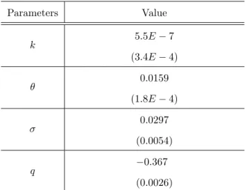
The parameter estimation results are presented in Table 2 with standard errors in parenthesis17_.

Table 2: Parameter estimates for one-factor model

Parameters Value

k 5:5E 7

(3:4E 4) 0:0159 (1:8E 4)

0:0297 (0:0054)

q 0:367

(0:0026)

All parameters, except k, are statistically signi…cant. The parameter k being statistically

insigni…cant with a t-statistic of 0:001 implies that the process does not tend to revert to its long-run mean but rather ‡uctuate like a random walk. Concerning the parameterq, following

the argument of Coxet al. (1985) negative values forq correspond to positive risk premia. The

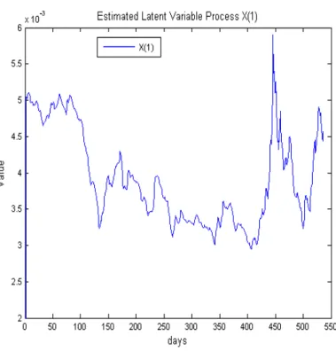
resulting process for the latent variable is presented in Figure 4.

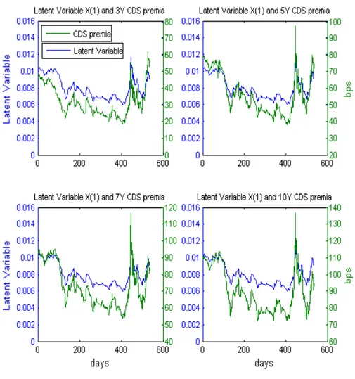
An interesting note can be made about the volatility parameter of the process . Given that

the model is estimated with a single factor, its movements should closely resemble the movements

in CDS premia which is exactly the case, though with much greater volatility18_{. This is illustrated}

in Figure 5

6.2 Two-Factor Intensity Model

Similar to the one-factor model, equation 21 with two latent variablesX1 and X2 was estimated

with a Kalman Filter on four CDS premia across 537 days of timeseries. As expected, adding an

extra latent variable signi…cantly improved the overall …t of the model with the correspondingR2

statistic for each of the four maturities at 95%, 89%, 98% and 99% respectively. The parameter

estimates are presented in the Table 3

1 7_{Standard erros are derived from the Fisher Information matrix.}

1 8_{The standard deviation of the latent process is an incredible}₀:₀₂₉_{when compared to the values for the standard}

(24)

Figure 4: Estimated process for the latent variableX1.

Table 3: Parameter estimates for two-factor model

Parameters Value

k1

0:004 (1:6E 5)

k2

0:014 (1:2E 5)

1

0:043 (1:1E 5)

2

0:011 (1:0E 5)

1

0:502 (1:9E 5)

2

0:092 (5:9E 6)

q1

0:012 (7:6E 6)

q2

(25)

Figure 5: Comparison of the estimated latent variable process with the four CDS premia.

Focusing on the estimates of the parameters. k1 and k2 are very close to zero implying slow

mean reversion of latent variables to their long-term means 1 and 2 while exhibiting signi…cant

volatility, with 1 and 2 well above the volatilities observed for CDS premia, as in the one-factor

model.

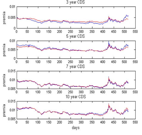
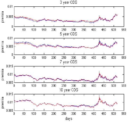
Figure 6 illustrates the …t of the model at various maturities across the whole timeseries. It is

interesting to note that the improvement in …t is signi…cant over the one-factor model, especially

at shorter 3 and 5 year maturities as well as at the end of the sample where greater turbulence can

be observed.

When estimating a model with two variables a modest di¢culty arises with the random part

of the discretized CIR process (Ft in equation 21) not found in the one-factor model. As it has been noted in the introductory section, by construction, the CIR process does not out rule the

possibility of getting ambiguous negative variances and this is exactly the case with the two factor

(26)

Figure 6: Four graphs showing the …t of the two-factor model at various terms of CDS premia across the timeseries. The blue line represents the observed values and the red the estimated values.

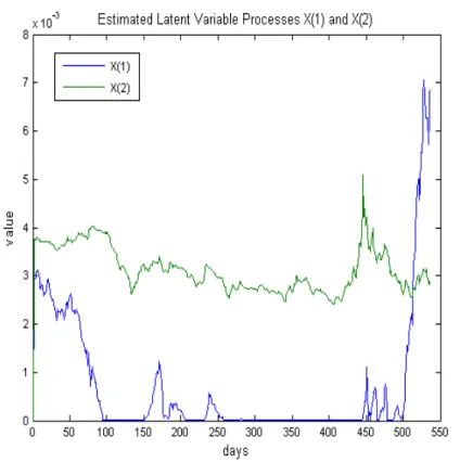
Although ambiguous, a zero value for a latent variable throughout a signi…cant part of the

timeseries can be justi…ed as follows. By construction, latent variables are uncorrelated and are

driven by some economic forces. Therefore it might occur that the forces driving one of the variables

cease to exist, or cancel each other out for a prolonged period of time. The second latent variable

seems to come into play with signi…cant and sudden jumps in CDS premia as the ones witnessed

in July of 2007 and the following months, in the Figures 7 corresponds to sample number 400

onwards.

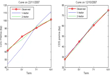
In Figure 8 a comparison between the …t of the models to CDS curves is presented. The two

graphs have been chosen where the average error of the one-factor model is largest (597.19 basis

points) and smallest (7.19 basis points) respectively.

At these two sample dates the improve in …t by adding a second factor into the model is evident.

(27)

Figure 7: Estimated processes for the latent variablesX1 and X2. As can bee see the 1st latent variable spent a signi…cant of the sample at its lower barrier …xed at0.

where the one-factor model performs quite well, the average error is further improved from 7.19

bp to 5.97 bp. Furthermore, by computing a log-likelihood ratio as 2L2 2L1 = 190219, and comparing it against the critical value of13:27 taken from the chi-squared distribution with four degrees of freedom (equal to the number of additional parameters in the two-factor model) and

percentile of 99%, I conclude that a second factor improves the …t of the model and is necessary

to account for the variations at the lower end of the curve.

6.3 Model Implied Probabilities of Default

From the construction of the model in equation 9 it is evident that the probability of default is an

essential ingredient to calculating the value of a CDS premia for a given maturity. Furthermore

as the probability of default in the estimated model depends solely on a set of latent variables, it

becomes theoretically possible to extract the implied risk-neutral probabilities of default from the

observed CDS premia as well as compute their evolution.

The average implied risk-neutral probabilities of default for the 3, 5, 7 and 10 year maturities

are presented in Table 4

(28)

Figure 8: Two graphs showing the relative …t of the one-factor model (blue line) and the two-factor model (green line) together with observed values for the CDS curve.

Table 4: Model implied risk-neutral probabilities of default

Term One-Factor Model Two-Factor Model

3Y 0:021 0:022

5Y 0:054 0:057

7Y 0:118 0:117

10Y 0:308 0:230

Both one-factor and two-factor models agree quite closely on most of the probabilities, one

exception being at the 10-year maturity. I must stress, however, that these probabilities of default

are computed from the risk-neutral measure Q that can di¤er substantially from the subjective

(real world) default probabilities, or the historic default probabilities published by rating agencies.

Berndt et al. (2005) conducted an extensive study comparing the relation between risk-neutral

probabilities implied by models studied in this paper and subjective probabilities calculated by

Moody’s. Their …ndings suggest that the ratio between the two can exhibit substantial volatility

and rise from2 at shorter maturities up to6 for longer maturities.

Results in this paper con…rm these large deviations between the two measures, where the ratio

of risk-neutral and average historic default probabilities of the entities composing the iTraxx20 _are

2:63,3:00,4:18and5:48for the 3, 5, 7 and 10 year maturities respectively.

2 0_{Historic default probabilities were computed …rst by calculating the average rating composition of the entities in}

(29)

7 Conclusions and Directions for Future Research

In the …rst few sections of this paper I presented a concise review of the two modeling approaches

most widely used in credit risk modeling: Structural models, directly linking the probabilities of a

…rm’s default to its internal structure, and more recent Intensity models, to which a …rm’s internal

structure is of no importance. I further concluded that, in a market with imperfect information

structural models are a special case of broader Intensity models.

A general Intensity model was parametrized with an a¢ne intensity, where the intensity is a

function of a set of latent variables following uncorrelated CIR di¤usion processes. This model

was then adapted to …t the CDS payment structure at four maturities and two sets of models

were estimated with a Kalman Filter approach on timeseries comprising 537 day observations. A

model with one latent variable for the intensity process demonstrated encouraging results for the

three longest maturities, however lacking in …t for the shortest, 3 year maturity. By adding an

additional latent variable it signi…cantly improved the …t of the model to account for 95%, 89%,

98% and 99% of variations at the lowest to highest maturities respectively. A number of di¢culties

were encountered during the estimation, namely a linearized version of the model had to be used

due to the Kalman Filter’s inability to handle non-linearity. Additionally in a two-factor model a

lower bound of zero had to be imposed on the second latent variable in order to avoid ambiguous

negative volatilities.

Further research could extend the results in this paper mainly in two ways. Firstly, by studying

the relation between estimated latent and macroeconomic / …nancial variables in an attempt to

establish a link between the CDS curve and real variables. Secondly, to use the model implied

default probabilities together with an external source of subjective probabilities to infer on the

evolution of risk premia.

8 Appendices

8.1 Feynman-Kac Approach

Feynman-Kac formula tells us that the expected value of an exponential function can be computed

as a solution to a partial di¤erential equation.

Theorem 1 21_{The Feynman-Kac Formula. Let}₍_{f; R}₎₂_Rn _Rn _and

f(Xt; T t) =Et

h

e RtTR(Xs)dsf(X_T;0)

i

(23)

(30)

then

@f

@(T t) = Af Rf (24)

f(x;0) = f(X ;0) (boundary condition)

moreover if a bounded function w(x; T t) solves above di¤erential equation and its associated

boundary condition, then it is an admissible solution f(x; T t) = w(x; T t). The parameter

Af is also said to be an in…nitesimal generator of the functionf.

In general the solution to the partial di¤erential equation is not trivial albeit in a few special

cases. A¢ne speci…cation of parameters is one of these special cases for which a solution to the

PDE is known in closed form. For an intuitive de…nition of a generator it helps to imagine some

functionf(Xt; t) that depends on the evolution of some stochastic processXt, now if we apply Ito’s lemma to calculate df(Xt;t)

dt we should come to a result who’s …rst component is deterministic and the second component is purely random. For an in…nitesimal interval of time, an in…nitesimal

generator is the part of this resulting function that if removed leaves us with a martingale. An

in…nitesimal generator of a Lévy process inRn _{can be found in Du¢e}_{et al.} _{(2000) and is outlined} in the following Proposition

Proposition 2 For a Lévy process of the form dXt= (Xt)dt+ (Xt)dBt+ dZt with vector

dimensions :D !Rn_, _:_D _!_Rn _Rn_{, jump probability} _{and a …xed jump size distribution}

on Rn governing the jump sizesz. An in…nitesimal generator of a function f(Xt; t) takes the

form

Af= (x)@f

@x + 1 2 n X i=1

(x)0 (x) @f

2

@x@x _i+ (x) Z

Rn

[f(x+z) f(x)]d (z) (25)

If all parameters in the model are of a¢ne dependence such as

(Xt) = 0+ 1Xt (26)

(Xt) = 0+ 1Xt (27)

R(Xt) = 0+ 1Xt (28)

(Xt) = l0+l1Xt (29)

then the in…nitesimal generator is also of a¢ne form and thus the Feynman-Kac formula can be

applied to obtain a partial di¤erential equation. Furthermore as described in Du¢e (2005) and

(31)

equations if the solution of the term structure model takes the form

f(Xt; T t) =e (T t)+ (T t)Xt (30)

where ( )and ( )for =T t solve the following di¤erential equations

d ( )

d = 0 0 ( )

1 2 ( )

0

0 ( ) l0( ( ( )) 1) (31)

d ( )

d = 1 1 ( )

1 2 ( )

0

1 ( ) l1( ( ( )) 1) (32)

where ( ( )) =R_Rne ( )zd (z)determines the jump-size distribution

8.2 Kalman Filter Optimization Algorithm

The Kalman Filter optimization algorithm is constructed from two blocks:

A Non-linear Kalman Filter for computing estimates of the latent variables at each time

period of the sample with a given set of parameters in the transition and measurement

equation;

A quasi-Newton optimization routine maximizing the maximum likelihood function and

ad-justing the parameter set in the transition and measurement equation.

The two blocks above are executed iteratively until an optimum is reached.

8.2.1 Kalman Filter Block

For a two-dimensional case with a model composed of two latent variables the measurement and

transition equations are

Xt = 1 e k +e kXt 1+Ft (33)

ct = H(Xt) +Rt (34)

Given that matrixH(Xt)in the measurement equation is a non-linear function of latent vari-ables it must …rst be linearized. Linearization is done by di¤erentiating the matrix with respect to

each of theXtthus constructing to what normally is referred to as the Jacobian matrix that I will denote /H_t. With the linearized version of the model and initial algorithm parametersX^0= 0and

(32)

1 - Compute optimal KalmanGain

Kt=Pt H/

0

t H/tPt H/

0

t+Rt 1

(35)

2 - Update latent variable estimates and compute the …lter error term

^

Xt = X^t +Kt ct H/X^t (36)

vt = ct H/X^t (37)

3 - Update estimate covariancePt. Calculate the …lter error covariance t and calculate the maximum likelihood valueLtbased on the assumption that …lter errors are normally distributed

Pt = (I KtH/t)Pt (38)

t = H/tPtH/

0

t+Rt (39)

Lt = ln [det ( t)] +vt0 tvt (40)

4 - Calculate optimal predictions for the covariance matrix, latent variables and recalculate the

linearization of matrixHt

P_t+1 = APtA

0

+Ft (41)

^

Xt+1 = AX^t (42)

/

H_t+1 = J acobian X^_t+1 (43)

Restart at no _{1 with}_P

t =Pt+1,X^t = ^Xt+1and /Ht=H/t+1

At the end of the iteration, when the last data point of the sample is reached, the maximum

likelihood function /Lis calculated as the sum of individual likelihood values

/

L=

T

X

t=1

Lt (44)

(33)

8.2.2 Optimization Block

For the optimization algorithm I used a preprogrammed matlab functionfmincon, details on which

can be found in online documentation at: http://www.mathworks.com. From online

documenta-tion:

fmincon uses a sequential quadratic programming (SQP) method. In this method,

the function solves a quadratic programming (QP) subproblem at each iteration. An

estimate of the Hessian of the Lagrangian is updated at each iteration using the BFGS

formula.

After a new set of parameters is chosen they are fed back into the Kalman Filter Block where

the maximum likelihood is calculated and sent back to the Optimization Block. This process is

repeated until no further improvement in …t is attainable.

8.3 Kalman Filter Linearization Methods

Consider the Kalman Filter measurement equation with a non-linear matrixH(Xt)inXt

ct=H(Xt) +Rt (45)

Being a Kalman Filter linear by construction, in its original form, it has not been made to

handle non-linear models proposed here. However a non-linear version of the …lter, the Extended

Kalman Filter can be applied by linearizing theH(Xt)through calculation of its …rst derivatives with respect to Xt (commonly known as the Jacobian). There is, however, a small detail to the linearization technique, as it must be chosen around which values the derivatives should be

evaluated. Apparently there are three alternatives with di¤erent levels of complexity and computer

time execution. In this paper I make use of the third alternative that demonstrated fair trade-o¤

between the speed of execution and parameter estimates.

The …rst one (at times referred to as the Extended Kalman Filter), being also the most computer

time consuming, is to calculate the Jacobian at each step and evaluate around the latest estimates

for Xt. This can be problematic during the …rst steps while the …lter is still converging to its steady state and divergence can arise if initial values were provided inaccurately, or if there is a

sudden rise in volatility of the observable variables.

The second one, is as time consuming as the …rst one, but that does not tend to diverge as often.

Here the Jacobian is calculated at each step, but evaluated around the latent variable long-run

(34)

mean of the process remains constant at each step, thus reducing the volatility of the Jacobian

values at each step.

The third one (at times referred to as the Linearized Kalman Filter), and the least time

con-suming, is to calculate the Jacobian only once around the long-run mean at the beginning of the

…lter. With this, time consumption can be reduced by the order of thousands. Assuming that in

the …rst two alternatives the …lter requires around 500 iterations to converge and takes 10 seconds

for each iteration, then with this alternative the number of iterations can be decreased to around

200 and the time to around 1 second. The main disadvantage is that it can lead to poor estimates

of the Jacobian matrix and in turn poor estimates of the path for the latent variable.

From the three alternatives described above, the …rst one seems to be the most commonly used.

Du¤ee (1999) and Chen & Scott (2003) made use of the …rst alternative in their study on interest

rate yield-curves. The third alternative is regularly published in technical books on engineering. I

did not …nd any study con…rming the use of the second alternative.

8.3.1 Negativity Problem in Kalman Filter

By choosing the CIR process as the underlying process for latent variables, one is inevitably

confronted with a problem of negative variance22 _{in the Kalman …lter transition equation (equation}

22). Negative volatility, additionally causes the maximum likelihood to go into the complex domain.

There are three solutions to this problem, two theoretical and the third one purely technical.

The …rst solution to the negativity problem and the one employed by Du¤ee (1999) and

dis-cussed as viable in Chen & Scott (2003) is to simply reset all the negative values of latent variables

to zero when they arise. This causes zero to function as a re‡ection barrier, however in practical

terms it happens so that zero works as an absorber for the latent variable, when reached, the latent

variable can stay there for a signi…cant period of time. A possible interpretation is that the forces

responsible for movements in the latent variable either cancel each other, or cease to exist for a

certain period of time.

The second solution, as discussed in the original paper on CIR processes by Coxet al. (1985)

is to impose a Kuhn-Tucker type restriction on parameters. The authors argue that by imposing

2k 2 _{on each latent variable process, the upward drift is su¢ciently large to make the origin} inacessible, in other words, an initial non-negative value for the latent variable can never

subse-quently become negative. In practice, however, a number of studies23 _{suggest that this condition}

2 2_{By construction, in the CIR di¤usion process the value of the latent variable a¤ects the volatility through a}

square-root, thus negative values for the latent variable inevitably cause the process to go into the complex domain. 2 3_{Studies with models including more than one latent variable tend to indicate relatively low values for the}

(35)

is rarely satis…ed when confronteda posteriori due to low values ofk and for at least one latent

variable in a multi-factor model.

A third, purely technical solution is for the numerical optimization routine used in the …lter to

cancel optimization when a negative value is encountered, assume the parameter as not viable and

retry with a new set. This solution can potentially have a drastic e¤ects on the optimization routine.

The optimization routine is constructed to receive a feedback from the estimation routine for

every choice of parameters and the value of this feedback determines the next choice of parameter

values. However if the feedback is returned, for example, as a binary value, then there is no way

to determine by how much the previous values should be adjusted in order to improve the …t of

the model.

8.4 Principal Component Analysis of the CDS Curve

Principal components and their contribution to the explanatory power of the CDS curve were

estimated using the matlabprincomp function. For details on the workings of this function refer

to the product documentation available at: http://www.mathworks.com

Figure 9: The bars on the graph represent the total contribution of each principal component to the explanatory power of the variances in the iTraxx Hi-Vol CDS curve. Vertical axes on the right shows the total variance explaned by both components.

Matlab code for calculating principal components and plotting the graph in Figure 9 is presented

(36)

%% Clear all variables from memory

clear all

clc

%% Load data

% Structure: Time series in lines - Maturities in columns

load(’itraxx.mat’);

%% Calculate Principal components

[pcs,newdata,variances,t2] = princomp(diff(itraxx./10000)); % Compute principal

components on 1st diferences

percent_explained = 100*variances/sum(variances); % Percentage of variance explained

by each component

cumulative_explained = cumsum(percent_explained) % Cumulative variance explained

by each component

%% Plot Results

figure, pareto(percent_explained)

xlabel(’Principal Component’)

ylabel(’Variance Explained (%)’)

8.5 Estimation Program

Here I will provide a rough outline of the scripts used in estimating the one-factor model. The

two-factor model shares the same set of equations, only di¤ering in the number of variables. The

program is composed of 3 matlab scripts that interact with each other during estimation, and 2

matrices containing data with CDS premia and risk-free interest rates.

8.5.1 Script estim.m

From this script the estimation process is launched. Care should be taken to execute the script

in blocks, to avoid ambiguous results. The …rst block loads two matrices into memory and sets

initial value for parameters. The second block executes a test run to make sure that all of the

information is available. The third block is responsible for the actual optimization. In the fourth

and …fth blocks statistics are calculated and …gures are plotted.

% Code should be run sequentially in blocks

%% 1st block

(37)

warning(’off’,’MATLAB:singularMatrix’);

warning(’off’,’MATLAB:nearlySingularMatrix’);

global y; %set the CDS premia variables to be available in all scripts

global rc; %set the interest rates to be available in all scripts

load(’cdsdata.mat’); %load the initial matrix with CDS premia

y = (cdsdata/10000)’; clear cdsdata %set CDS premia to matrix y

load(’rc40.mat’); %load interest rates

p(1) = 5.4481e-007; % k1, speed of convergence (transition equation)

p(2) = 0.015884; % b1, long-run mean (transition equation)

p(3) = 0.029705; % s1, volatility (transition equation)

p(4) = -0.36725; % q1, risk premium (measurement equation)

%% 2nd block - Test Routine

% This block returns

% mlerr - current maximum likelihood

% ky - estimated CDS premia

% kx - estimated latent variable time-series

% kv - model errors

% kxest - estimated (anterior) latent variable time-series

% pdefault - prob. default implicit in each CDS maturity

[mlerr, ky, kx, kv, kxest, pdefault] = estimateproc(p);

%% 3rd block - Optimization Routine

% This block finds the minimum of the maximum likelihood function

% careful as it is very computer and time intensive. To stop execution

% press Ctrl-C

% pvar - at the end of execution return the standard errors^2

A = []; b = []; Aeq = []; beq = [];

lb = [0; 0; 0; -1];

ub = [1; 5; 5; 0];

nonlcon = [];

options = optimset(’MaxIter’,50000,’MaxFunEvals’,3000,’DiffMinChange’,1e-07,’DiffMaxChange’,1e-01);

% optimization options

[pest,fval,exitflag,output,lambda,grad,hessian] = fmincon(@estimateproc,p,A,b,Aeq,beq,lb,ub,nonlcon,

(38)

pvar = inv(hessian); % Var-Covar matrix of the estimates = inv(fisher matrix): hessian

= Fisher Information Matrix

warning(’on’,’MATLAB:nearlySingularMatrix’);

warning(’on’,’MATLAB:singularMatrix’);

%% 4th block - Figures

% Prints out some graphs

CDStxt = [3;5;7;10];

figure,

for k = 1:4

subplot(4,1,k)

plot(y(k,20:length(y))); hold on; plot(ky(k,20:length(ky)),’r’); hold off

title([’CDS(’,num2str(CDStxt(k)),’) actual(blue) vs. estimated(red)’])

end

clear k

clear sse sse R

%% 5th block - R2 Statistic

% Calculates R^2

for k = 1:4

for i = 1:length(y)

sse(k,i) = (y(k,i)*10000-ky(k,i)*10000)^2; % Sum of Squared Errors

sst(k,i) = (y(k,i)*10000-mean(y(k,:))*10000)^2; % Total Sum of Squares

end

R(k) = sum(1-sse(k,:)/sst(k,:)); % R^2

end

8.5.2 Script estimateproc.m

This script can only be executed from withinestim.mand is responsible for executing the Kalman

Filter routine and calculating the maximum likelihood value. Due to the non-linearity of model

there is a third script (calcjacobian.m) that is called to calculate the Jacobian matrix of the

measurement equation 21.

function [mlerr, ky, kx, kv, kxest, pdefault] = estimateproc(p)

tic

global y;

(39)

nsimul = length(y);

% Set of parameters affecting both

c = 0;

k1 = p(1);

b1 = p(2);

s1 = p(3);

q1 = p(4);

dt = 1/360; % Actual days in a year

T = [3 5 7 10]; % Array of CDS maturities

l = 0.40; % Loss Given Default (LGD)

%%%%%%%%%%%%%%%%%%%%%%%%%%%%%%%

% Transition equation variables

A = [exp(-k1*dt)];

d = [b1*(1-exp(-k1*dt))];

R = [1e-7 0 0 0; 0 1e-7 0 0; 0 0 1e-7 0;0 0 0 1e-7];

%%%%%%%%%%%%%%%%%%%%%%%%%%%%%

% kalman initial variables

% The purpose of these variable is to allocate memory and make sure that no

% operation is done on a non existent variable

%kxmin = [0.1; 0.1];

kxmin = 0.01; % anterior latent variable estimates (initial state)

kx = 0; % latent variable estimates

ky = y(:,1); % observed CDS premia

Pmin = s1^2; % anterior kalman P matrix

P = 0; % kalman P marix

I = 1; % identity marix for the univariate case

kv = zeros(4,1); % CDS estimation error

pdefault = 0; % probability of default

kxest = 0; % latent variables estimated values

sigmaM = 0; % sigma matrix

L = zeros(1,length(y)); % log-likelihood

broke = 0; % control variable. When =1 --> the process broke due to

convtol = 1; % control variable

(40)

%% Simple 1 time linearization around [b1 b2]

%[kyhat Hj] = calcjacobian(T,[k1 k2],c,l,[b1 b2],[b1; b2],i);

[kyhat Hj pdef] = calcjacobian(T,k1,c,l,b1,b1,q1,s1,1,3); % only spits out Hj with

kyhat = 0

%% Kalman loop

for i = 1:nsimul

% Jump through the first iteration in order to execute the next

% iteration with a full set of parameters

if i <= convtol

continue

end

%%%%%%%%%%%%%%%%%%%%%%%%%%%%%%

% Calculate Estimation Error %

kv = y(:,i) - Hj*kxmin;

%%%%%%%%%%%%%%%%%%%

% Calculate Sigma %

% Sigma is used as input parameter in the 1st step and in the maximum

% log-likelihood function

sigmaM = Hj*Pmin*Hj’+R; %if det(sigmaM) < 0; dbstop in estimateproc.m at 46; end

invsigmaM = inv(sigmaM);

L(i) = log(det(sigmaM)) + kv’*invsigmaM*kv; if i == 2; L(i-1) = L(i); end

if ~isreal(L(i)); broke = 1; break; end % reset complex values to 0

%%%%%%%%%%%%%%%%%%%%%%%%%%%%%%

% Calculate Var-Covar Matrix %

% This is the var-covar marix of the Transition equation

Q = [((s1^2)*(kx(1)*(exp(-k1*dt)-exp(-2*k1*dt))+(b1/2)*(1-exp(-k1*dt))^2))/k1];

%%%%%%%%%%%%

% 1st step %

(41)

K = Pmin*Hj’*invsigmaM;

%%%%%%%%%%%%

% 2nd step %

% two alternatives can be used: either use an aproximate value for

% ’kyhat’ as Hj*kxmin; or recalculate kyhat each time which consumes

% quite a lot of time

%kx = kxmin + K*(y(:,i) - kyhat);

kx = kxmin + K*(y(:,i) - Hj*kxmin);

if kx(1) < 0; kx(1) = 0; end % reset to 0 negative kx

%%%%%%%%%%%%

% 3rd step %

%

P = (I - K*Hj)*Pmin;

%%%%%%%%%%%%

% 4th step %

%

kxmin = d + A*kx;

Pmin = A*P*A’ + Q;

%%%%%%%%%%%%%%%%%%%%%%%%%%%%%%%

% Calculate output parameters %

% kyhat --> estimated CDS spread

% pdefault --> estimated probability of default at each maturity

% kxest --> estimated latent variable

%[kyhat Hj pdef] = calcjacobian(T,k1,c,l,b1,kx,q1,s1,i,3); %Comment during optimization.

Jacobian around current latent variable value

%[kyhat Hj] = calcjacobian(T,k1,c,l,b1,b1,q1,s1,1,2); % Jacobian & kyhat around

b1 --> long-term trend

%%%%%%%%%%%%%%%%%%%%%%%%

INSTITUTO SUPERIOR DE ECONOMIA E GESTÃO

UNIVERSIDADE TÉCNICA DE LISBOA