Higher statistical moments and an outlier detection technique as two alternative methods that capture long-term changes in continuous environmental data

(1)

HESSD

11, 4729–4751, 2014

Long-term changes in environmental data

I. Arismendi et al.

Title Page

Abstract Introduction

Conclusions References

Tables Figures

◭ ◮

Back Close

Full Screen / Esc

Printer-friendly Version Interactive Discussion

Discussion

P

a

per

|

D

iscussion

P

a

per

|

Discussion

P

a

per

|

Discuss

ion

P

a

per

|

Hydrol. Earth Syst. Sci. Discuss., 11, 4729–4751, 2014 www.hydrol-earth-syst-sci-discuss.net/11/4729/2014/ doi:10.5194/hessd-11-4729-2014

Hydrology and Earth System

Sciences

Open Access

Discussions

This discussion paper is/has been under review for the journal Hydrology and Earth System Sciences (HESS). Please refer to the corresponding final paper in HESS if available.

Higher statistical moments and an outlier

detection technique as two alternative

methods that capture long-term changes

in continuous environmental data

I. Arismendi1, S. L. Johnson2, and J. B. Dunham3

1

Department of Fisheries and Wildlife, Oregon State University, Corvallis, Oregon, 97331, USA

2

US Forest Service, Pacific Northwest Research Station, Corvallis, Oregon, 97331, USA

3

US Geological Survey, Forest and Rangeland Ecosystem Science Center, Corvallis, Oregon, 97331, USA

Received: 11 April 2014 – Accepted: 23 April 2014 – Published: 13 May 2014 Correspondence to: I. Arismendi (ivan.arismendi@oregonstate.edu)

(2)

HESSD

11, 4729–4751, 2014

I. Arismendi et al.

Title Page

Tables Figures

◭ ◮

Back Close

Full Screen / Esc

Discussion

P

a

per

|

D

iscussion

P

a

per

|

Discussion

P

a

per

|

Discuss

ion

P

a

per

|

Abstract

Central tendency statistics may not capture relevant or desired characteristics about the variability of continuous phenomena and thus, they may not completely track tem-poral patterns of change. Here, we present two methodological approaches to iden-tify long-term changes in environmental regimes. First, we use higher statistical mo-5

ments (skewness and kurtosis) to examine potential changes of empirical distributions at decadal scale. Second, we adapt an outlier detection procedure combining a non-metric multidimensional scaling technique and higher density region plots to detect anomalous years. We illustrate the use of these approaches by examining long-term stream temperature data from minimally and highly human-influenced streams. In par-10

ticular, we contrast predictions about thermal regime responses to changing climates and human-related water uses. Using these methods, we effectively diagnose years with unusual thermal variability, patterns in variability through time, and spatial variabil-ity linked to regional and local factors that influence stream temperature. Our findings highlight the complexity of responses of thermal regimes of streams and reveal a diff er-15

entiated vulnerability to both the climate warming and human-related water uses. The two approaches presented here can be applied with a variety of other continuous phe-nomena to address historical changes, extreme events, and their associated ecological responses.

1 Introduction

20

Variability is a fundamental feature that shapes ecological and evolutionary processes, yet most traditional statistics tend to be based on overly simplistic assumptions about variability. For example, many commonly used statistical approaches depend on the assumptions of normality and equality of variance, hardly the norm in nature. Applica-tion of such methods requires the use of statistical transformaApplica-tions (e.g., logarithmic or 25

(3)

HESSD

11, 4729–4751, 2014

I. Arismendi et al.

Title Page

Tables Figures

◭ ◮

Back Close

Full Screen / Esc

Discussion

P

a

per

|

D

iscussion

P

a

per

|

Discussion

P

a

per

|

Discuss

ion

P

a

per

|

variability. This issue is particularly troublesome for understanding temporally contin-uous phenomena, where measures of central tendency (e.g., the mean or median) convey little information about the overall pattern of variability. Indeed, previous stud-ies have illustrated the importance of understanding continuous phenomena based on their temporal patterns (Colwell, 1974) and the behavior of extremes (Gaines and 5

Denny, 1993), rather than traditional descriptors of central tendency.

Here, we explore two approaches that quantify and visualize changes in empirical distributions of continuous environmental variables over time focusing on natural phe-nomena that can be described as “regimes”. Typically regimes are quantified in terms of the magnitude, frequency, duration, and timing of events, which seems simple enough, 10

but such has not been the case in practice. Consider, for example, the case of stream flow regimes, where well over 150 partially redundant statistical descriptors have been derived (Olden and Poff, 2003). To complicate matters further, such regimes can be partitioned further into di_fferent temporal frames or grains (e.g., Steel and Lange, 2007; Arismendi et al., 2013a). If one wishes to efficiently provide an overall description of 15

a regime or to envision changes in regimes over time without resorting to a plethora of descriptors, the solutions are not immediately obvious.

We use two approaches to address the general problem of describing regimes and their temporal changes, using thermal regimes of streams as an illustrative example. First, using frequency analysis we examine patterns of variability and long-term shifts 20

in stream temperature using higher statistical moments (skewness and kurtosis) of em-pirical distributions by season across decades. Second, we combine non-metric mul-tidimensional scale ordination technique (N-MDS) and highest density regions (HDR) plots to detect anomalous years. To illustrate the utility of these approaches, we ap-ply them to contrast predictions and questions about long-term responses of thermal 25

(4)

HESSD

11, 4729–4751, 2014

I. Arismendi et al.

Title Page

Tables Figures

◭ ◮

Back Close

Full Screen / Esc

Discussion

P

a

per

|

D

iscussion

P

a

per

|

Discussion

P

a

per

|

Discuss

ion

P

a

per

|

Thermal regime of streams as an illustrative example

Temperature is a fundamental driver of ecosystem processes in freshwaters (Shelford, 1931; Fry, 1947; Magnuson et al., 1979; Vannote and Sweeney, 1980). Short-term (daily/weekly/monthly) descriptors of mean and maximum temperatures during sum-mertime are frequently used for characterizations of thermal habitat availability and 5

quality (McCullough et al., 2009), definitions of regulatory thresholds (Groom et al., 2011), and predictions about possible influences of climate change on streams (Mohseni et al., 2003; Mantua et al., 2010; Arismendi et al., 2013a, b). These sim-ple descriptors can serve as useful first approximations, but do not capture the full range of thermal conditions that the aquatic biota experience at daily, seasonal, or an-10

nual intervals (see Poole and Berman, 2001; Webb et al., 2008). Both human impacts and climate change have been shown to affect thermal regimes of streams at a variety of temporal scales, across seasons or years (e.g., Steel and Lange, 2007; Arismendi et al., 2012, 2013a, b). For example, the recent warming climate may lead to different responses of streams that may not be captured only using average or maximum tem-15

perature values (Arismendi et al., 2012). Daily minimum stream temperatures in winter are showing more warming than daily maximum values during summer (Arismendi et al., 2013a; for air temperatures see Donat and Alexander, 2012). In human modified streams, seasonal shifts in stream temperatures and earlier warmer temperatures have been recorded following removal of riparian vegetation (Johnson and Jones, 2000). 20

However, simple threshold descriptors cannot characterize these shifts. Using the first approach (higher statistical moments), we examine the question of whether a recent warming climate has led a shift in the shape of the stream temperature distribution or if stream temperature has simply moved entirely to the right without any change in shape. In addition, we compare these potential shifts in the distribution of stream 25

(5)

HESSD

11, 4729–4751, 2014

I. Arismendi et al.

Title Page

Tables Figures

◭ ◮

Back Close

Full Screen / Esc

Discussion

P

a

per

|

D

iscussion

P

a

per

|

Discussion

P

a

per

|

Discuss

ion

P

a

per

|

examine if those anomalous years represent a regional influence of the climate or al-ternatively highlight the importance of local factors. Previous studies have shown that detecting long-term changes of thermal regimes of streams is complex and the use of only traditional statistical approaches may mislead a variety of responses of ecological relevance (Arismendi et al., 2013a, b).

5

2 Material and methods

2.1 Study sites and time series

We selected long-term gage stations (US Geological Survey and US Forest Service) that monitored year-round daily stream temperature in Oregon, California, and Idaho (n₌10; Table 1). The sites were selected based on (1) availability of continuous daily 10

records for at least 31 years (1 January 1979 to 31 December 2009) and (2) com-plete information for time series of daily minimum (min), mean (mean), and maximum (max) stream temperature for at least 93 % of the period of record. Half of the sites (n₌5) were located in unregulated streams (sites 1–5) and the other half were in regulated streams (sites 6–10). Regulated streams were those with reservoirs con-15

structed before 1978. Time series were carefully inspected and for the outlier analysis only (see below) we interpolated missing data following Arismendi et al. (2013a). The percentage of daily missing records of each time series was less than 7 %. To ensure enough observations to adequately represent the tails of the respective distributions at a seasonal scale for analyses of higher statistical moments (i.e., winter: December– 20

(6)

HESSD

11, 4729–4751, 2014

I. Arismendi et al.

Title Page

Tables Figures

◭ ◮

Back Close

Full Screen / Esc

Discussion

P

a

per

|

D

iscussion

P

a

per

|

Discussion

P

a

per

|

Discuss

ion

P

a

per

|

2.2 Higher statistical moments

To compare stream temperatures across sites, we standardized time series of daily temperature values using a Z-transformation as follows:

STi =

T_i−µ σ

5

where ST_i was the standardized temperature at dayi,T_i was the actual temperature value at dayi (◦C),µwas the mean andσwas the standard deviation of the respective time series considering the entire time period.

Higher statistical moments of skewness and kurtosis are often considered problem-atic in parametric statistics, where data is often assumed to be normal. In reality, how-10

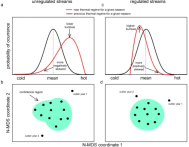
ever, these moments can be useful to describe changes in environmental variables over long-term periods (see Shen et al., 2011; Donat and Alexander, 2012). Skewness addresses the question of whether or not a certain variable is symmetrically distributed around its mean value. With respect to temperature, positive skewness of the distribu-tion or skewed right indicates colder condidistribu-tions are more common (Fig. 1c) whereas 15

negative skewness or skewed left represents increasing prevalence of warmer condi-tions (Fig. 1a). Therefore, increases in the skewness over time could occur with in-creases in warm conditions, dein-creases in cold conditions, or both.

Kurtosis describes the structure of the distribution between the center and the tails representing the dispersion around its “shoulders”. In other words, as the probabil-20

ity mass decreases around its shoulders it may increase in either the center, or the tails, or both resulting in a rise in the peakedness, the tailweight, or both and thus, the dispersion of the distribution around its shoulders increases. The reference stan-dard is zero, a normal distribution with excess kurtosis equal to kurtosis minus three (mesokurtic). A sharp peak in a distribution that is more extreme than a normal distribu-25

(7)

HESSD

11, 4729–4751, 2014

I. Arismendi et al.

Title Page

Tables Figures

◭ ◮

Back Close

Full Screen / Esc

Discussion

P

a

per

|

D

iscussion

P

a

per

|

Discussion

P

a

per

|

Discuss

ion

P

a

per

|

tails. A distribution with tails more flattened than the normal distribution (excess kurto-sis below zero) described higher frequencies spread across the tails (platykurtic). With respect to temperature, a leptokurtic distribution may indicates that average conditions are much more frequent and there is a lower proportion of both extremes cold and warm values (Fig. 1c). A platykurtic distribution represents a more evenly distributed 5

distribution across all values with a higher proportion of both extreme cold and warm values (Fig. 1a). Therefore, increases in the kurtosis over time would occur with de-creases in extreme conditions, inde-creases of average conditions, or both.

Skewness and excess kurtosis are dimensionless and were estimated as follows:

Skewness₌ n

(n−1)(n−2)

Xn

i=1

_T

i−µ

σ

3

10

Kurtosis=

"

n(n₊1) (n−1)(n−2)(n−3)

Xn

i=1

_T

i−µ

σ

4#

− 3(n−1)

2

(n−2)(n−3)

wherenrepresented the number of records of the time series,T_i was the temperature of the dayi,µandσthe mean and standard deviation of the time series.

To define the status of the skewness for the stream temperature distribution in a par-15

ticular season and decade, we used two criteria. First, we classified the amount of skewness in three categories following Bulmer (1979): “highly skewed” (if skewness was <−1 or >1), “moderately skewed” (if skewness was between −1 and −0.5 or between 0.5 and 1), and “symmetric” (if skewness was between−0.5 and 0.5). Sec-ond, we statistically tested whether the skewness coefficient was different from zero 20

following Cramer (1998):

SES=

s

6n(n−1) (n−2)(n+1)(n+3)

Z_Skewness₌Skewness

(8)

HESSD

11, 4729–4751, 2014

I. Arismendi et al.

Title Page

Tables Figures

◭ ◮

Back Close

Full Screen / Esc

Discussion

P

a

per

|

D

iscussion

P

a

per

|

Discussion

P

a

per

|

Discuss

ion

P

a

per

|

where SES was the standard error of skewness,Z_Skewness the test statistic, andnthe number of records of the time series. The critical value ofZ_Skewnesswas approximately 2 (two-tailed test of skewness6=0 at significance level of 0.05). IfZ_Skewnesswas<−2, the temperature distribution was likely skewed negative (“negative skewed”), if Z_Skewness

was >2, the temperature distribution was likely skewed positive (“positive skewed”). 5

However, if Z_Skewness was between −2 and 2 we could not reject the null hypothesis that the distribution was skewed (“non-significant”). We also used similar procedures to test whether the excess kurtosis was different from zero following (Cramer, 1998):

SEK=2(SES)

s

(n2₋₁₎

(n−3)(n+5)

Z_Kurtosis=Skewness SEK 10

where SES was the standard error of skewness, SEK the standard deviation of ex-cess kurtosis,Z_Kurtosisthe test statistic, andnrepresented the number of records of the time series. IfZ_Kurtosis was<−2, the temperature distribution likely had “negative ex-cess kurtosis or platykurtic”, ifZ_Kurtosis was>2, the temperature distribution likely had 15

“positive excess kurtosis or leptokurtic”. Finally, ifZ_Kurtosis was between−2 and 2, we could not reject the null hypothesis (“non-significant”). We computed higher statistical moments using R ver. 2.15.1 (R Development Core Team, 2012).

2.3 Outlier detection procedure

We explored and examined features expressed by thermal regimes of streams, which 20

(9)

HESSD

11, 4729–4751, 2014

I. Arismendi et al.

Title Page

Tables Figures

◭ ◮

Back Close

Full Screen / Esc

Discussion

P

a

per

|

D

iscussion

P

a

per

|

Discussion

P

a

per

|

Discuss

ion

P

a

per

|

temperatures for each day within a year across all years. The N-MDS analysis places each year in a multivariate space in the most parsimonious arrangement (relative to each other) with no a priori hypotheses. Based on an iterative optimization procedure (999 random starts) we minimize a measure of disagreement or stress between their distances in 2-D (for a detailed explanation see Kruskal, 1964). The resulting coordi-5

nates 1 and 2 from the 2-D plot provided a collective index of how unique a given year was (Fig. 1b and d). In N-MDS the order of the axes was arbitrary and the coordinates represented no meaningful absolute scales for the axis. Fundamental to this method is the relative distances apart of points with a higher proximity indicating a higher degree of similarity, whereas more dissimilar points are positioned further apart. We performed 10

the N-MDS analyses using the software Primer ver. 6.1.15 (Clarke, 1993; Clarke and Gorley, 2006).

Using the two coordinates of each point (year) from the 2-D plot originated in the N-MDS ordination procedure, we created a bivariate high dimensional region (HDR) box-plot (Hyndman, 1996). The HDR plot has been typically produced using the two 15

main principal component scores from a traditional principal component analysis (PCA) (Hyndman, 1996; Chebana et al., 2012). However, is this study, we modified this pro-cedure taking the advantage of the higher flexibility and lack of assumptions of the N-MDS analysis (Everitt, 1978; Kenkel and Orloci, 1986) to provide the two coordi-nates needed to create the HDR plot. In the HDR box-plot, there are regions defined 20

based on a probability coverage (e.g., 50; 90; or 95 %) where all points (years) within the probability coverage region have higher density estimates than any of the points outside the region (Fig. 1b and d). The outer-region of the probability coverage region is bounded by points representing anomalous years (in Fig. 1b and d see outlier years). We created the HDR plots using the package “hdrcde” (Hyndman et al., 2012) in R ver. 25

(10)

HESSD

11, 4729–4751, 2014

I. Arismendi et al.

Title Page

Tables Figures

◭ ◮

Back Close

Full Screen / Esc

Discussion

P

a

per

|

D

iscussion

P

a

per

|

Discussion

P

a

per

|

Discuss

ion

P

a

per

|

3 Results

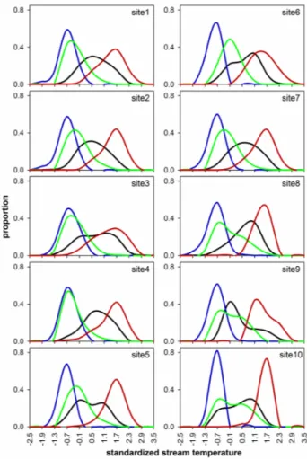
Stream temperature empirical distributions were distinctive among seasons, but sea-sons were relatively similar across sites (Fig. 2). Winter had the narrowest range and highest frequency of observations at colder standardized temperature categories (−1.3, −0.7). The second highest proportion of observations in the year were also 5

colder values occurring during spring in unregulated streams and during summer at four of the five regulated sites. This shift of frequency was likely due to release of warmer water from the reservoir management upstream. Temperature distributions during winter had high overlap with those during spring. Fall distributions showed broadest range, with a similar proportion for a number temperature values.

10

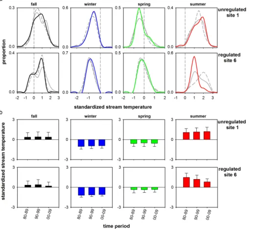
Changes in the shape of empirical distributions among seasons over decades were not immediately evident, but the state of skewness and kurtosis captured this changes in cases when lower statistical moments (average and standard deviation) did not show differences (e.g., site 1 during fall and summer in Fig. 3; Tables 2 and 3; Supple-ment). The utility of combining skewness and kurtosis to detect changes in distribu-15

tional shapes over time is illustrated by unregulated sites 1 and 2 during fall (Tables 2 and 3; Supplement). At these sites, there were shifts between the last two decades from negatively skewed to more symmetrical distributions and from mesokurtic to platykurtic states suggesting a proportion of the probability mass moved from center into the tails due to recent less extreme cold and more warm conditions. Overall, in most unregu-20

lated sites, kurtosis changed its state with recent increases during winter, summer, and spring (Table 3; Supplement). Winter and summer mostly had negatively skewed distri-butions whereas spring generally had positively skewed distridistri-butions or those with little change across decades, except for site 3 (Table 2; Supplement). Decadal changes in both skewness and kurtosis during winter and summer observed in unregulated sites 25

(11)

HESSD

11, 4729–4751, 2014

I. Arismendi et al.

Title Page

Tables Figures

◭ ◮

Back Close

Full Screen / Esc

Discussion

P

a

per

|

D

iscussion

P

a

per

|

Discussion

P

a

per

|

Discuss

ion

P

a

per

|

shoulders apparently due to decreases in the importance of extreme colder conditions. Collectively, these findings illustrate how higher statistical moments may describe the complexity of temporal changes in stream temperature among seasons and highlight how shifts may occur at different portions of the distribution (e.g., extreme cold, aver-age, or warm conditions).

5

In regulated sites, we observed shifts toward colder temperatures (e.g., sites 6 and 9 during summer and fall in Fig. 3; Supplement) suggesting local influences of wa-ter regulation mask climate-related impacts. This illustrated mixed effects of skewness and kurtosis due to climate and water regulation, especially during spring, winter, and summer (Tables 2 and 3; Fig. 3; Supplement). In particular, in spring, patterns of skew-10

ness were similar to unregulated sites whereas patterns of kurtosis were in opposite directions (more platykurtic in regulated sites). This can be explained by the water dis-charged from reservoirs in spring that was a mix of the cool inflows to the reservoir, the cold water stored in the reservoir itself from the winter, and yet the surface of the reser-voir warmed because of increasing solar radiation. Patterns of skewness and kurtosis 15

seen in regulated sites also highlights the influences of site-dependent water manage-ment coupled with climatic influences. This is illustrated by the skewness of sites 7 and 8 compared to sites 9 and 10 in winter (Table 2) and the high variability of the state of skewness among sites in summer.

Outliers representing years (Fig. 4; Supplement) were identified as points outside 20

95 % confidence intervals (CI). During the period (1979–2009), year 1992 was identi-fied as an outlier at five sites (or eight sites at 90 % CI) and years 1987 and 2008 were outliers in four sites. Most unregulated sites had between two and four outlier years (or between four and five at 90 % CI), whereas regulated sites had two or less (or between three and four at 90 % CI, except site 10 which had seven), a result consistent with the 25

(12)

HESSD

11, 4729–4751, 2014

I. Arismendi et al.

Title Page

Tables Figures

◭ ◮

Back Close

Full Screen / Esc

Discussion

P

a

per

|

D

iscussion

P

a

per

|

Discussion

P

a

per

|

Discuss

ion

P

a

per

|

The outlier-detection method captured years with anomalies in either magnitude or timing of events (Fig. 4; Supplement). For example, year 1992 and 1987 were outliers likely due to magnitude of warming throughout year. In other sites, such as unregulated sites 3, 4 and 5, the outlier years were most likely due to increased temperatures in seasons other than summertime, and not related to higher summertime temperatures. 5

4 Discussion

Here we show the utility of using higher statistical moments and outlier detection as alternative approaches to capture long-term changes in empirical distributions of en-vironmental regimes and whether if these changes are consistent across site types. Stream ecosystems are exposed to multiple climatic and non-climatic forces which 10

may differentially affect their hydrological regimes (e.g., temperature and streamflow). In particular, we show that potential timing and magnitude of responses of stream tem-perature to both the recent warming climate and other human-related impacts vary among seasons, years, and across sites. Central tendency statistics may or may not capture these alterations on thermal regimes which could be relevant to infer their eco-15

logical and management implications. For example, by increasing both extreme cold and warm conditions, but maintaining average values. Increased understanding of the shape of empirical distributions by season or year will also help researchers and re-source managers evaluate potential impacts of shifting environmental regimes on or-ganisms and processes across a range of disturbance types. Empirical distributions 20

are a simple, but comprehensive way to examine high frequency measurements that include the full range of values. Higher statistical moments provide useful information to characterize and compare regimes and can show which season could be most re-sponsive to disturbances. This could help improve predictive models of climate change impacts by incorporating full regimes into scenarios.

25

(13)

HESSD

11, 4729–4751, 2014

I. Arismendi et al.

Title Page

Tables Figures

◭ ◮

Back Close

Full Screen / Esc

Discussion

P

a

per

|

D

iscussion

P

a

per

|

Discussion

P

a

per

|

Discuss

ion

P

a

per

|

single metrics are used to describe environmental regimes they have to be selected and thus, information must be compressed. Often selection means simplification re-sulting in the compression or loss of information (e.g., Arismendi et al., 2013a). By examining the whole empirical distribution of temperature we can provide a better char-acterization of shifts over time or following other disturbances than simple thresholds 5

or descriptors. In particular, our findings suggest a differential resilience of unregulated streams to the recent warming climate that could be likely related to local conditions of watersheds (e.g., Arismendi et al., 2012). Regulated and unregulated sites located in the same watershed (sites 2, 7, and 8 in Table 1 and Supplement) may share similar outlier years (e.g., year 2008 as a cold-water outlier) suggesting strong climatic influ-10

ences during those years. However, when sites are spatially located close to one an-other (unregulated sites 3 and 4 in Table 1) they may not necessarily share the same outlier years (they share only year 1987) likely because local drivers may be more important than regional climate forces. By using the outlier detection technique, we il-lustrate their utility to describe regional vs. local influences of climate on streams. For 15

example, a differential vulnerability of streams to regional or local climate changes by characterizing years with extreme conditions or those when seasonal shifts occurred.

In conclusion, our two approaches complement traditional summary statistics by helping to explain long-term continuous environmental variable behaviors for seasons and years. We illustrate this using temperature of streams in unregulated and regulated 20

sites as an example. In particular, we show water regulation may mask climate related influences. Using cold-water mountain streams from similar regions, we characterize responses and changes in thermal regimes that are useful in representing the influ-ences of both local impacts and regional climatic forcing. Although we did not include a broad range of stream types, our analysis of stream temperatures within the set of 25

(14)

HESSD

11, 4729–4751, 2014

I. Arismendi et al.

Title Page

Tables Figures

◭ ◮

Back Close

Full Screen / Esc

Discussion

P

a

per

|

D

iscussion

P

a

per

|

Discussion

P

a

per

|

Discuss

ion

P

a

per

|

air temperature see Shen et al., 2011). These analyses will be useful to characterize how regimes of continuous phenomena have changed in the past, may respond in the future, or to identify the type and timing of their resilience.

Supplementary material related to this article is available online at http://www.hydrol-earth-syst-sci-discuss.net/11/4729/2014/

5

hessd-11-4729-2014-supplement.pdf.

Acknowledgements. Brooke Penaluna provided comments on the manuscript and Vicente

Monleon revised statistical concepts. Part of the data was provided by the HJ Andrews Ex-perimental Forest research program, funded by the National Science Foundation’s Long-Term Ecological Research Program (DEB 08-23380), US Forest Service Pacific Northwest Research

10

Station, and Oregon State University. Financial support for IA was provided by US Geological Survey, the US Forest Service Pacific Northwest Research Station and Oregon State Univer-sity through joint venture agreement 10-JV-11261991-055. Use of firm or trade names is for reader information only and does not imply endorsement of any product or service by the US Government.

15

References

Arismendi, I., Johnson, S. L., Dunham, J. B., Haggerty, R., and Hockman-Wert, D.: The paradox of cooling streams in a warming world: regional climate trends do not parallel variable local trends in stream temperature in the Pacific continental United States, Geophys. Res. Lett., 39, L10401, doi:10.1029/2012GL051448, 2012.

20

Arismendi, I., Johnson, S. L., Dunham, J. B., and Haggerty, R.: Descriptors of natural thermal regimes in streams and their responsiveness to change in the Pacific Northwest of North America, Freshwater Biol., 58, 880–894, 2013a.

Arismendi, I., Safeeq, M., Johnson, S. L., Dunham, J. B., and Haggerty, R.: Increasing syn-chrony of high temperature and low flow in western North American streams: double trouble

25

(15)

HESSD

11, 4729–4751, 2014

I. Arismendi et al.

Title Page

Tables Figures

◭ ◮

Back Close

Full Screen / Esc

Discussion

P

a

per

|

D

iscussion

P

a

per

|

Discussion

P

a

per

|

Discuss

ion

P

a

per

|

Bulmer, M. G.: Principles of Statistics, Dover Publications Inc., New York, 1979.

Chebana, F., Dabo-Niang, S., and Ouarda, T. B. M. J.: Exploratory functional flood frequency analysis and outlier detection, Water. Resour. Res., 48, W04514, doi:10.1029/2011WR011040, 2012.

Clarke, K. R.: Nonparametric multivariate analyses of changes in community structure, Aust. J.

5

Ecol., 18, 117–143, 1993.

Clarke, K. R. and Gorley, R. N.: PRIMER v6: User Manual/Tutorial, PRIMER-E, Plymouth, 2006.

Colwell, R. K.: Predictability, constancy, and contingency of periodic phenomena, Ecology, 55, 1148–1153, 1974.

10

Cramer, D.: Fundamental Statistics for Social Research: Step-by-step Calculations and Com-puter Techniques Using SPSS for Windows, Routledge, London, 1998.

Donat, M. G. and Alexander, L. V.: The shifting probability distribution of global daytime and night-time temperatures, Geophys Res Lett., 39, L14707, doi:10.1029/2012GL052459, 2012.

15

Everitt, B.: Graphical Techniques for Multivariate Data, North-Holland, New York, 1978. Fry, F. E. J.: Effects of the Environment on Animal Activity, University of Toronto Studies,

Bi-ological Series 55, Publication of the Ontario Fisheries Research Laboratory, 68, Toronto, Canada, 1–62, 1947.

Gaines, S. D. and Denny, M. W.: The largest, smallest, highest, lowest, longest, and shortest:

20

extremes in ecology, Ecology, 74, 1677–1692, 1993.

Groom, J. D., Dent, L., Madsen, L. J., and Fleuret, J.: Response of western Oregon (USA) stream temperatures to contemporary forest management, Forest Ecol. Manage., 262, 1618–1629, 2011.

Hyndman, R. J.: Computing and graphing highest density regions, Am. Stat., 50, 120–126,

25

1996.

Hyndman, R. J., Einbeck, J., and Wand, M.: Package “hdrcde”: Highest Density Regions and Conditional Density Estimation, available at: http://cran.r-project.org/web/packages/hdrcde/ hdrcde.pdf (last access: 15 January 2014), 2012.

Johnson, S. L. and Jones, J. A.: Stream temperature response to forest harvest and debris

30

flows in western Cascades, Oregon, Can. J. Fish. Aquat. Sci., 57, 30–39, 2000.

(16)

HESSD

11, 4729–4751, 2014

I. Arismendi et al.

Title Page

Tables Figures

◭ ◮

Back Close

Full Screen / Esc

Discussion

P

a

per

|

D

iscussion

P

a

per

|

Discussion

P

a

per

|

Discuss

ion

P

a

per

|

Kruskal, J. B.: Non-metric multidimensional scaling: a numerical method, Psychometrika, 29, 115–129, 1964.

Magnuson, J. J., Crowder, L. B., and Medvick, P. A.: Temperature as an ecological resource, Am. Zool., 19, 331–343, 1979.

Mantua, N., Tohver, I., and Hamlet, A.: Climate change impacts on streamflow extremes and

5

summertime stream temperature and their possible consequences for freshwater salmon habitat in Washington State, Climatic Change, 102, 187–223, 2010.

McCullough, D. A., Bartholow, J. M., Jager, H. I., Beschta, R. L., Cheslak, E. F., Deas, M. L., Ebersole, J. L., Foott, J. S., Johnson, S. L., Marine, K. R., Mesa, M. G., Petersen, J. H., Souchon, Y., Tiffan, K. F., and Wurtsbaugh, W. A.: Research in thermal biology: burning

10

questions for coldwater stream fishes, Rev. Fish. Sci., 17, 90–115, 2009.

Mohseni, O., Stefan, H. G., and Eaton, J. G.: Global warming and potential changes in fish habitat in US streams, Climatic Change, 59, 389–409, 2003.

Olden, J. D. and Poff, N. L.: Redundancy and the choice of hydrologic indices for characterizing streamflow regimes, River Res. Appl., 19, 101–121, 2003.

15

Poole, G. C. and Berman, C. H.: An ecological perspective on in-stream temperature: natural heat dynamics and mechanisms of human-caused thermal degradation, Environ. Manage., 27, 787–802, 2001.

R Development Core Team: R: A Language and Environment for Statistical Computing, avail-able at: http://www.R-project.org, R Foundation for Statistical Computing, Vienna, Austria„

20

2012.

Shelford, V. E.: Some concepts of bioecology, Ecology, 123, 455–467, 1931.

Shen, S. S. P., Gurung, A. B., Oh, H., Shu, T., and Easterling, D. R.: The twentieth century contiguous US temperature changes indicated by daily data and higher statistical moments, Climatic Change, 109, 287–317, 2011.

25

Steel, E. A. and Lange, I. A.: Using wavelet analysis to detect changes in water temperature regimes at multiple scales: effects of multi-purpose dams in the Willamette River basin, River Res. Appl., 23, 351–359, 2007.

Vannote, R. L. and Sweeney, B. W.: Geographic analysis of thermal equilibria: a conceptual model for evaluating the effects of natural and modified thermal regimes on aquatic insect

30

communities, Am. Nat., 115, 667–695, 1980.

(17)

HESSD

11, 4729–4751, 2014

I. Arismendi et al.

Title Page

Tables Figures

◭ ◮

Back Close

Full Screen / Esc

Discussion

P

a

per

|

D

iscussion

P

a

per

|

Discussion

P

a

per

|

Discuss

ion

P

a

per

|

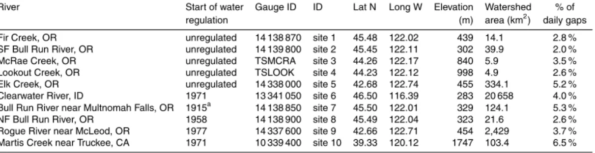
Table 1.Location and characteristics of unregulated (n₌5) and regulated (n₌5) streams at

the gaging sites. Percent of gaps in the stream temperature time series from January 1979 to December 2009 used in this study.

River Start of water Gauge ID ID Lat N Long W Elevation Watershed % of regulation (m) area (km2) daily gaps

Fir Creek, OR unregulated 14 138 870 site 1 45.48 122.02 439 14.1 2.8 % SF Bull Run River, OR unregulated 14 139 800 site 2 45.45 122.11 302 39.9 2.0 % McRae Creek, OR unregulated TSMCRA site 3 44.26 122.17 840 5.9 3.5 % Lookout Creek, OR unregulated TSLOOK site 4 44.23 122.12 998 4.9 2.6 % Elk Creek, OR unregulated 14 338 000 site 5 42.68 122.74 455 334.1 5.2 % Clearwater River, ID 1971 13 341 050 site 6 46.50 116.39 283 20 658 4.0 % Bull Run River near Multnomah Falls, OR 1915a _{14 138 850} _{site 7} _45.50 _122.01 ₃₂₉ _124.1 _{5.3 %}

NF Bull Run River, OR 1958 14 138 900 site 8 45.49 122.04 323 21.6 2.6 % Rogue River near McLeod, OR 1977 14 337 600 site 9 42.66 122.71 454 2,429 3.7 % Martis Creek near Truckee, CA 1971 10 339 400 site 10 39.33 120.12 1747 103.4 6.5 %

(18)

HESSD

11, 4729–4751, 2014

I. Arismendi et al.

Title Page

Tables Figures

◭ ◮

Back Close

Full Screen / Esc

Discussion

P

a

per

|

D

iscussion

P

a

per

|

Discussion

P

a

per

|

Discuss

ion

P

a

per

|

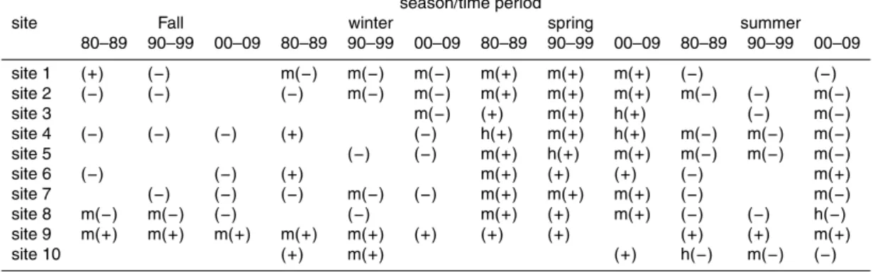
Table 2.Magnitude and direction of the state of skewness in probability distributions of daily

minimum stream temperature by season and decade at unregulated (sites 1–5) and regulated (sites 6–10) streams. Symmetric distributions and non-significant skewed distributions are not indicated. m₌moderately skewed; h₌highly skewed; (−)₌negatively skewed; (₊)₌positively skewed (see Supplement for more details).

season/time period

site Fall winter spring summer

80–89 90–99 00–09 80–89 90–99 00–09 80–89 90–99 00–09 80–89 90–99 00–09

(19)

HESSD

11, 4729–4751, 2014

I. Arismendi et al.

Title Page

Tables Figures

◭ ◮

Back Close

Full Screen / Esc

Discussion

P

a

per

|

D

iscussion

P

a

per

|

Discussion

P

a

per

|

Discuss

ion

P

a

per

|

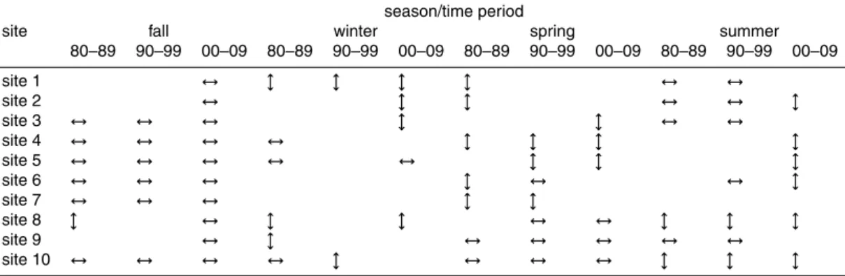
Table 3.State of kurtosis of probability distributions of daily minimum stream temperature by

season and decade at unregulated and regulated sites. Platykurtic distributions are indicated by “↔” and leptokurtic distributions indicated by “l”. Mesokurtic distributions and non-significant kurtosis of distributions are not shown (see Supplement for more details).

season/time period

site fall winter spring summer

80–89 90–99 00–09 80–89 90–99 00–09 80–89 90–99 00–09 80–89 90–99 00–09

site 1 ↔ l l l l ↔ ↔

site 2 ↔ l l ↔ ↔ l

site 3 ↔ ↔ ↔ l l ↔ ↔

site 4 ↔ ↔ ↔ ↔ l l l l

site 5 ↔ ↔ ↔ ↔ ↔ l l l

site 6 ↔ ↔ ↔ l ↔ ↔ l

site 7 ↔ ↔ ↔ l l

site 8 l ↔ l l ↔ ↔ l l l

site 9 ↔ l ↔ ↔ ↔ ↔ ↔

(20)

HESSD

11, 4729–4751, 2014

I. Arismendi et al.

Title Page

Tables Figures

◭ ◮

Back Close

Full Screen / Esc

Discussion

P

a

per

|

D

iscussion

P

a

per

|

Discussion

P

a

per

|

Discuss

ion

P

a

per

|

Fig. 1.Conceptual diagram showing hypothesized long-term responses of water temperature

(21)

HESSD

11, 4729–4751, 2014

I. Arismendi et al.

Title Page

Tables Figures

◭ ◮

Back Close

Full Screen / Esc

Discussion

P

a

per

|

D

iscussion

P

a

per

|

Discussion

P

a

per

|

Discuss

ion

P

a

per

|

Fig. 2.Density plots of standardized temperatures (1979–2009) by season (winter – blue line;

(22)

HESSD

11, 4729–4751, 2014

I. Arismendi et al.

Title Page

Tables Figures

◭ ◮

Back Close

Full Screen / Esc

Discussion

P

a

per

|

D

iscussion

P

a

per

|

Discussion

P

a

per

|

Discuss

ion

P

a

per

|

Fig. 3.Examples of (a)density plots of standardized temperatures by decade (period 80–89

(23)

HESSD

11, 4729–4751, 2014

I. Arismendi et al.

Title Page

Tables Figures

◭ ◮

Back Close

Full Screen / Esc

Discussion

P

a

per

|

D

iscussion

P

a

per

|

Discussion

P

a

per

|

Discuss

ion

P

a

per

|

Fig. 4.Examples of (left) bivariate HDR boxplots and (right) standardized daily temperature