ISSN 1941-7020
© 2009 Science Publications
Solving the State Assignment Problem Using Stochastic
Search Aided with Simulated Annealing
Walid M. Aly
Technical and Vocational Institute, Arab Academy for Science,
Technology and Maritime Transport, Alexandria, Egypt
Abstract: Problem statement: Solving the state assignment problem means finding the optimum assignment for each state within a sequential digital circuit. These optimum assignments will result in decreasing the hardware realization cost and increasing the reliability of the digital circuit. Unfortunately, the state assignment problem belongs to the class of nondeterministic polynomial time problems (NP complete) which requires heavy computations. Different attempts have been made towards solving the problem with reasonable recourses. Approach: This study presented a methodology for solving the state assignment problem, the methodology conducted a neighborhood search while using a heuristic to determine the fitness of solution. To avoid being trapped at a local optimum solution, a metaheuristic (simulated annealing) was utilized for deciding whether a new solution should be accepted. A case study was included to demonstrate the proposed procedure efficiency. Results: The proposed approach finds the optimum assignment for the case study. Conclusion: In this study, we explored the usage of a stochastic search technique inspired by simulated annealing to solve the problem of the state assignment problem. This proved the efficiency of the methodology.
Key words: Simulated annealing, digital circuit design, state assignment
INTRODUCTUION
Designing a synchronous sequential digital logic circuit is a hard task that requires a different numbers of stages to be accomplished efficiently so that the produced design will approach an optimum design.
The whole digital system can be recognized as a Finite State Machine (FSM), where the digital system encounter a finite number of states, that the information in each state would describe adequately the system and the output can be evaluated at such a state.
If the output of the system can be evaluated based on the present state only, the system is designated as a Moore machine, however if the output depends on both the current state and the system input, the system is designated as a
Mealy machine.
The design procedure for designing a sequential circuit can be described as follows[1]:
• Originating from the written description of the design problem, both the number of distinct states (S1, S2,….Sn) and the rules of transition between states are identified. A state diagram and a state table is the output of this stage. The "implication table" method can be used to eliminate redundant states so that the number of states needed to describe the system is minimal
• Each state is assigned a unique string of binary numbers, this step is our main concern
• Based on the type of flip-flops used to realize the digital system, Karnaugh maps are drawn for each input to the flip-flops used so that the state table is valid
One of the main factors that affect the cost of the hardware realization of a sequential logic circuit is the binary string assignment chosen for each state. Different assignments can be applied, finding the assignment that will produce the minimum cost for hardware realization means solving the State Assignment Problem (SAP).
Each state is represented as a string of 0 and 1 s, the length of the string that will represent each state is calculated by:
L = ceil(log2n) (1)
Where:
L = String length n = Number of states
ceil(x) = Mathematical function returning first positive integer higher than X
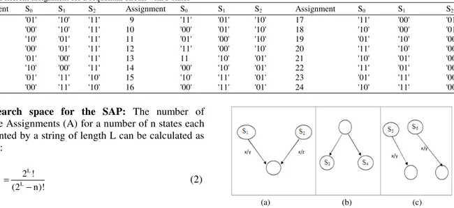
Table 1: Different assignment for a sequential circuit with 3 states
Assignment S0 S1 S2 Assignment S0 S1 S2 Assignment S0 S1 S2
1 '01' '10' '11' 9 '11' '01' '10' 17 '11' '00' '01'
2 '00' '10' '11' 10 '00' '01' '10' 18 '10' '00' '01'
3 '10' '01' '11' 11 '01' '00' '10' 19 '01' '10' '00'
4 '00' '01' '11' 12 '11' '00' '10' 20 '11' '10' '00'
5 '01' '00' '11' 13 11 '10' '01' 21 '10' '01' '00'
6 '10' '00' '11' 14 '00' '10' '01' 22 '11' '01' '00'
7 '01' '11' '10' 15 '10' '11' '01' 23 '01' '11' '00'
8 '00' '11' '10' 16 '00' '11' '01' 24 '10' '11' '00'
The search space for the SAP: The number of possible Assignments (A) for a number of n states each represented by a string of length L can be calculated as follows:
L n
L L
2
2 !
A C
(2 n)!
= =
− (2)
The number of assignments is actually a very large number; a 16 states problem will have a 2.0923e+013 different assignments. Table 1 shows the 24 possible assignments that can be applied to a 3 states problem.
Some of these state assignments are equivalent to each other[2], two state assignments are considered equivalent, if one of them can be produced by permuting any of its columns. Removing the equivalent state assignment leaves only the distinct state assignment whose number can be calculated by Eq. 3:
L
distinct L (2 )! A
L!(2 n)!
=
− (3)
If symmetrical flip flops like T or J-K are used, two state assignments are also considered equivalent, if one of them can be produced by complementing any of its columns, this reduces the number of distinct states to be:
L
distinct L
(2 1)!
A
L!(2 n)!
− =
− (4)
Even with this search space reduction, the number of different state assignments is still large and for a state assignments problem with 10 states, the number of possible assignments is more than 7e07. With this vast search space, the SAP belongs to the class of NP complete problems[3], where the resources needed to solve the problem increase very quickly as the size of problem grows. An arbitrary choice is easy and will always work, however it may require a lot of extra logic.
(a) (b) (c)
Fig. 1: Heuristic rules for state assignment
Several attempts have been made to solve the SAP[4], Newton[5] introduces an exact algorithm that minimize the number of product terms, Micheli et al.[6] propose an algorithm knows as KISS (keep internal state simple), recently nontraditional techniques like evolutionary algorithms were also attempted[7,8], none of these approached had provided a deterministic algorithm for solving the problem.
In real world, different hard computational problems exist where there are no exact applicable algorithm that is guaranteed to find the optimum solution in reasonable time and using reasonable resources. For these types of complex problems heuristics and Metaheuristics are usually used.
Heuristics for state assignments: Finding the optimum solution for the SAP means trying all the assignments using a Karnaugh map for each input to the flip-flops and then calculating the number of literals and gates that appeared in the logic expression. This would require a huge amount of time. With 7 flip-flops, checking all unique assignments would take 10193 years at one calculation/nano sec.
However, a heuristic exist to attempt to solve the SAP in a reasonable time, The basic idea[1] is that the some of the states are preferred to be adjacent, adjacency means having state assignments differing in only 1 bit. These states are:
• States having the same next state for the same input (Fig. 1a)
• The next states of a common state (Fig. 1b) • States with the same output for the same input
MATERIALS AND METHODS
The proposed methodology provides the steps for a stochastic search, as many stochastic search techniques are inspired by process found in nature, the search conducted is inspired by simulated annealing[9].
Simulated annealing is an analogy to the annealing in solids[10], the main theme is to start the search at a certain temperature and while conducting a search, this temperature start to cool down. If during a search a better solution is found it is accepted, a worse solution is probabilistically accepted with higher chance of acceptance at higher temperatures than at low temperatures, this simple-yet efficient-idea prevents the search from being trapped at a local optimum solution.
In our search, a random solution is created and then a neighborhood search is conducted for evolving new and hopefully better solution, the search procedures can be summarized as follows:
Step 1: Create a random candidate solution based on the number of states.
Step 2: Calculate the fitness of this solution.
Step 3: Apply neighborhood search to evolve a new solution.
Creating a random candidate solution: Each solution is coded as one dimensional array of binary bits, the length of array is equal to the number of states (n) multiplied by the number of bits required to designate each state (L), each L bits combine together to give the bit assignment of a state. Table 2 shows an example of solution 00101110 for a four states problem (S0, S1, S2 and S3).
A simple algorithm is used to create candidate solution by creating different random decimal numbers between 1 and (2L-1), then each state is assigned the binary equivalent of one of these numbers, state S0 is always assigned a series of zeros.
Fitness function: The fitness function would take a proposed assignment of states as an input and return a figure of merit representing how good this candidate solution is from the point of view of the applied heuristic.
This value reflects how much the candidate solution obeyed the three guidelines. These guide lines are translated to a number of rules defining which states
Table 2: Example for solution coding
S0 S1 S2 S3
00 10 11 10
should be adjacent to each other. Adjacent states mentioned in rules are grouped in groups, acceptable group sizes are 1, 2, 4, 8, or in general 2k cells where k is a positive number. 4 states are considered adjacent if each state of them is adjacent to 2 other states, similarly 8 states are considered adjacent if each state of them is adjacent to 3 other states.
Each candidate solution is checked against the whole set of rules and the fitness value is updated according to the following equation:
Misplaced
Fitness Fitness 1 (1* )
Groupsize
= + − (5)
where, misplaced is the number of states in the group within a certain rule that are not adjacent. Each fully obeyed rule will increase the fitness function by a total one.
Neighborhood search: The search can be described as follows:
• Starting from a current solution and current temperature, new solution from neighborhood is created; this is done randomly by flipping the state assignment of 2 states
• The process of creating a random solution is repeated for K iterations till K solutions are created • The candidate solution with the highest fitness is
pointed out of the K solution
• If this candidate solution has a higher fitness, it is accepted probabilistically based on the probability acceptance function
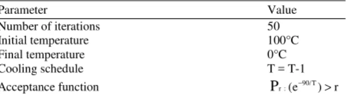
• Temperature is decreased according to cooling schedule, process repeats until temperature reaches zero or a solution is found that obeys all rules Table 3 shows the parameters of the simulated annealing metaheuristic used.
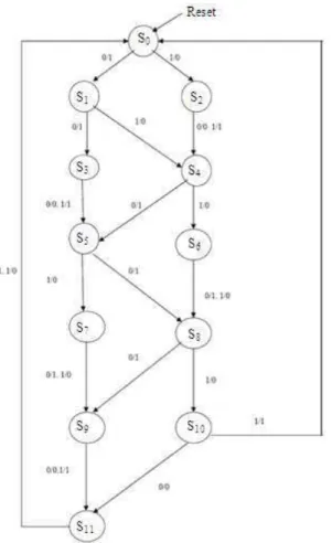
Practical example: The problem that will demonstrate the proposed methodology will be a 12 state problem, although 12 might seem as a small number, the search space is still huge (8.7178e+011), Fig. 2 shows the state diagram for the selected problem.
Table 3: simulated annealing parameters
Parameter Value
Number of iterations 50
Initial temperature 100°C
Final temperature 0°C
Cooling schedule T = T-1
Acceptance function 90/T
r :(e ) r
P − >
Fig. 2: State diagram
According to the mentioned guidelines, the following states should be adjacent:
First guideline:
(S1, S2), (S3, S4), (S5, S6), (S7, S8), (S9, S10), (S10, S11) Second guideline:
(S1, S2), (S3, S4), (S5, S6), (S7, S8), (S9, S10), (S11, S0) Third guideline:
(S0, S1, S4, S5, S6, S7, S8, S11) (S2, S3, S9, S10)
Based on the above and eliminating redundant rules, 9 distinguished rules should be obeyed to ensure that the solution is optimum. These rules where fed to software implementing the pre-described procedures.
RESULTS
The optimum solution obeying all rules was found to be as shown in Table 4.
Fig. 3: Fitness values
Table 4: Optimum solution
00 01 11 10
00 S0 S9 S3 S4
01 S11 S10 S2 S1
11 S6 S5
10 S7 S8
Fig. 3 shows the finesses of candidate solutions that were recorded at different temperature during the search.
DISCUSSION
The curve in Fig. 3 is a typical simulated annealing search curve, current fitness value was allowed to decrease probalistically until finally the optimum solution was found. The optimum solution was found at 8°C.
The obtained solution shown in Table 4 shows that the proposed procedure succeeded in finding the optimal assignment based on the given heuristic, this emphasis the efficiency of using nontraditional techniques- in our case simulated annealing- to solve a highly computational problem like SAP. The results are good enough to recommend and encourage future researches in investigating other nontraditional techniques with problems with a higher number of states.
CONCLUSION
guided by simulated annealing rules, so that the search would not be trapped at a local optimum point.
REFERENCES
1. Roth Jr., C.H., 1995. Fundamentals of Logic Design. 4th Edn., Wadsworth Publishing Company, ISBN: 10: 0534954723, pp: 770. 2. Harrison, M.A., 1968. On equivalence of state
assignments. IEEE Trans. Comput., 1: 55-57 3. Amaral, J.N., K. Tumer and J. Ghosh, 1992.
Applying genetic algorithms to the state assignment problem: A case study. Proc. SPIE Adapt. Learn. Syst., 1706: 2-13. DOI: 10.1117/12.139933
4. Ahmad, I. and M.K. Dhodhi, 2000. State assignment of finite-state machines. IEE Proc. Comput. Digit. Tech., 147: 15-22. DOI: 10.1049/ip-cdt:20000163
5. Devadas, S. and A.R. Newton, 1991. Exact algorithms for output encoding, state assignment and four level Boolean minimization. IEEE Trans. Comput. Aid. Des. Integrat. Circ. Syst., 10: 13-27. DOI: 10.1109/43.62788
6. De Micheli, G., R.K. Brayton and A. Sangiovanni-Vincentelli, 1985. Optimal state assignment for finite state machines. IEEE Trans. Comput. Aid. Des. Integrat. Circ. Syst., 4: 269-285. http://ieeexplore.ieee.org/xpl/freeabs_all.jsp?arnum ber=1270123
7. Chyzy, M. and W. Kosinski, 2002. Evolutionary algorithm for state assignment of finite state machines. Proceedings of the Euromicro Symposium on Digital System Design, (ESDSD’02), IEEE Xplore Press, USA., pp: 359-362. DOI: 10.1109/DSD.2002.1115392
8. Nedjah, N. and L.M. de Mourelle, 2005. Evolutionary synthesis of synchronous finite state machines. Stud. Fuzziness Soft Comput., 161: 103-127. DOI: 10.1007/3-540-32364-3_5
9. Russell, S.J. and P. Norvig, 1995. Artificial Intelligence: A Modern Approach. 1st Edn., Prentice Hall, New Jersey, ISBN: 10: 0131038052, pp: 932.