Variable Neighborhood Search based algorithms for high school timetabling

Variable Neighborhood Search based algorithms for high

school timetabling

George H.G. Fonseca

, Haroldo G. Santos

a

Computing and Systems Department, Federal University of Ouro Preto, Brazil b_{Computing Department, Federal University of Ouro Preto, Brazil}

a r t i c l e

i n f o

Available online 6 February 2014

Keywords:

Variable Neighborhood Search High School Timetabling Problem Third International Timetabling Competition

a b s t r a c t

This work presents the application of Variable Neighborhood Search (VNS) based algorithms to the High School Timetabling Problem. The addressed model of the problem was proposed by the Third International Timetabling Competition (ITC 2011), which released many instances from educational institutions around the world and attracted 17 competitors. Some of the VNS algorithm variants were able to outperform the winner of Third ITC solver, which proposed a Simulated Annealing– Iterated local Search approach. This result coupled with another reports in the literature points that VNS based algorithms are a practical solution method for providing high quality solutions for some hard timetabling problems. Moreover they are easy to implement with few parameters to adjust.

&2014 Published by Elsevier Ltd.

1. Introduction

The High School Timetabling Problem is faced by many educa-tional institutions around the world. The basic search version consists in assigning teacherclass activities to timeslots and rooms in such a way that no teacher, class or room is involved with more than one event at time. Generally, this assignment is repeated weekly until the end of the semester. Many other constraints are considered in real problems, like availability of teachers, to avoid idle times and to limit the number of lessons of the same subject taught to a class in a day. Beyond its practical importance, this problem was proven to be

NP Hard [1,2]. Progress in heuristic and exact approaches for tackling these problems is a major goal of current research in Operations Research and Artificial Intelligence.

Three international competitions (ITCs) were made to bring the attention of scientists and practitioners for this problem, with the objective of performing comparisons of different methods in a controlled computational environment: thefirst one happened in 2003[3]and was won by Kostuch[4]with a 3-phase Simulated Annealing (SA)[5]based approach. In 2007, the second one[6]

started and was composed of three separated tracks, which were mostly won by Müller[7]also with a Simulated Annealing based approach. The last one[8]happened in 2012 and was won by a Simulated Annealing–Iterated Local Search[9]approach.

As the results of the competitions show, local search methods are defining the state-of-art heuristic solvers for educational

timetabling problems. Specially, the Simulated Annealing meta-heuristic composed the solver of all winners. The role of exact methods which employ Integer Programming, such as the pro-posed in[10–12], appears to be still very limited for tackling the

problems and instances which appeared in these competitions, considering the absence of these techniques in submissions. This scenario contrasts with the first International Nurse Rostering Competition[13], for instance, where two of thefirst places used Integer Programming in some form.

This paper presents a computational study of Variable Neigh-borhood Search and its variants applied to the Third ITC problem. The results indicate that the proposed method outperforms the state-of-art method.

The remaining of this work is organized as follows:Section 2

presents the problem considered in this paper, the Third ITC problem; Section 3 presents our solution approach; Section 4

presents computational experiments and finally, Section 5 con-cludes our paper and discusses future works.

2. High School Timetabling Problem model

The roots of the School Timetabling model considered in this paper, the model of the Third ITC, are in the Benchmarking project for (High) School Timetabling.1 The project, which involved a group of researchers in this area, started with the ambitious goal of developing a XML format capable of modeling different school Contents lists available atScienceDirect

journal homepage:www.elsevier.com/locate/caor

Computers & Operations Research

http://dx.doi.org/10.1016/j.cor.2013.11.012 0305-0548&2014 Published by Elsevier Ltd.

E-mail addresses:george@decsi.ufop.br(G.H.G. Fonseca),

haroldo@iceb.ufop.br(H.G. Santos). 1

timetabling problems arising in diverse institutions around the world. Initial versions of this project appeared in the PATAT 2008 conference [14], with an improved version named XHSTT pub-lished later[15]. Nowadays, the project site holds approximately 50 datasets from 11 countries. The project site also includes an evaluator to validate solutions and the best known solutions are kept, so that the results of newly proposed methods can be immediately confronted with previously obtained results. Some of the previous models which are now in XHSTT are[16–20,10,21].

The model is split into three main entities: Time and Resources, Events and Constraints. A solution consists of a set of assignments of times and resources to the events.

2.1. Times and resources

The time entity consists of a timeslot, which is an indivisible interval of time. Timeslots do not overlap and can be grouped in timegroups. Resources are entities which attend events. Typical resources are students, teachers and rooms[21]:

Students: a group of students attends events (lessons); important

constraints associated with students are the control of their idle times and the number of lessons taken by day.

Teachers: teachers perform their academic tasks in events; the

allocation of teachers for specific teaching activities can be preassigned or not; when teachers are not preassigned, they should be assigned according to their qualifications and workload limits.

Rooms: the usage of rooms for hosting events must be observed:

some events require rooms with a given capacity and/or a set of special features.

2.2. Events

An event (instance event) is a meeting between resources, usually representing a simple lesson or a set of lessons (event group). Each instance event needs to be scheduled into one or

more solution events. Timeslot assignments to events are called

meetsand the assignment of resources to events istasks. The term

courseis used to designate a group of students who attend to the

same events. Other kinds of events, like meetings, are allowed by the model [21]. The following attributes can be specified for events, thefirst one is the only obligatory:

Duration:represents the number of timeslots which have to be

assigned to the event.

Course: a course is a grouping of events: events declared in the

same course constitute a course of study in one subject for one group of students.

Pre-assigned resources: to attend the event.

Workload: that will be added to the total workload of resources

assigned to the event.

Pre-assigned timeslot: some events have only one timeslot in which

they can be assigned.

2.3. Constraints

Post et al.[21]group the constraints into three categories: basic constraints of scheduling, constraints of events and constraints of resources. The objective function fðÞis computed considering the summation of penalties for deviations in different constraints and events/resources which they refer. Theflexibility of XHSTT allows the inclusion of non-linear terms in the cost function which is used to compute the penalties[15]. The constraints are also divided into hard

constraints, whose satisfaction is mandatory; and soft constraints, whose satisfaction is desirable but not obligatory. Costs for violations in these two types of constraints are summed in two separated costs: the infeasibility cost and the quality cost, defining a hierarchical objective function. Each instance can define whether a constraint is hard or soft, its weight and the type of cost function used (eg. linear or quadratic). For more details, see[15].

2.3.1. Basic constraints of scheduling

1. ASSIGNTIME: assign timeslots to each event.

2. ASSIGNRESOURCE: assign the resources to each event.

3. PREFER TIMES: indicates that some event have preference for a

particular timeslot(s).

4. PREFERRESOURCES: indicates that some event have preference for a

particular resource(s).

2.3.2. Constraints to events

1. LINKEVENTS: to schedule a set of events to the same starting time.

2. SPREAD EVENTS: specify the allowed number of occurrences for

event groups in time groups between a minimum a maximum number of times; this constraint can be used, for example, to define a daily limit of lessons.

3. AVOID SPLIT ASSIGNMENTS: for each event, assign a particular

resource to all of its meets.

4. DISTRIBUTE SPLITEVENTS: for each event, assign between a

mini-mum and a maximini-mum meets of a given duration.

5. SPLITEVENTS: limits the number of non-consecutive meets that

an event should be scheduled and its duration.

2.3.3. Constraints to resources

1. AVOIDCLASHES: assign the resources without clashes (i.e. without

assign the same resource to more than one event at a timeslot). 2. AVOIDUNAVAILABLETIMES: avoid assigning resources on the times

that they are not available.

3. LIMITWORKLOADCONSTRAINT: schedule the workload of the resources

between a minimum and a maximum bound.

4. LIMITIDLE TIMES: the number of idle times in each time group should lie between a minimum and a maximum bound for each resource; typically, a time group consists of all timeslots of a given week day.

5. LIMITBUSYTIMES: the number of busy times in each time group

should lie between a minimum and a maximum bound for each resource.

6. CLUSTERBUSYTIMES: the number of time groups with a timeslot assigned to a resource should lie between a minimum and a maximum limit; this can be used, for example, to concentrate teacher's activities in as few days as possible.

3. Solution approach

Our approach uses the Kingston High School Timetabling Engine (KHE)[22]to generate initial solutions. Afterwards, we implemented the Variable Neighborhood Search metaheuristic and some of its variants to perform local search around this solution. These elements will be explained in the following subsections.

3.1. Build method

the presented approach. This solver was chosen to generate the initial solutions since it is able to find reasonably good initial solutions in short amounts of time.

The incorporated solver is based on the concept of Hierarchical Timetabling[23], where smaller allocations are joined to generate bigger blocks of allocation until a full representation of the solution is developed. Hierarchical Timetabling is supported by the Layer Tree data structure [23], consisting of nodes that represent the required meet and task allocation. An allocation may appear in at most one node. A Layer is a subset of nodes having the propriety that none of them can be overlapped in time. Commonly, nodes are grouped in a Layer when share resources.

The hard constraints of the problem are modeled to this data structure and then a Matching problem is solved tofind the times/ resources allocation. The Matching is done by connecting each node to a timeslot or resource respecting the property of Layer. For full details, see[23,22].

3.2. Neighborhood structure

Six neighborhood structures were used:

1. Event Swap (ES): Two eventse₁ ande₂have their timeslotst₁

andt2swapped respectively.

2. Event Move (EM): An event e1 is moved from timeslot t1 to

another timeslott2.

3. Event Block Move (EBM): Works likeES, but when moving events

with different durations in contiguous timeslots, keeps these events adjacent.

4. Resource Swap (RS): Two eventse1ande2have their assigned

resourcesr1 andr2swapped respectively. Resourcesr1andr2

should play the same role to allow the swap (e.g. both have to be teachers).

5. Resource Move (RM): An evente1 has its assigned resourcer1

replaced by a new resourcer2.

6. Kempe Move (KM): Two timest₁andt₂arefixed and one seeks

the best path at the bipartite conflict graph containing all events int1andt2; arcs are built from conflicting events which are in different timeslots and their cost is the cost of swapping the timeslots of these two events.

The set of neighborhoods is quite similar to the one used in Fonseca[9].

3.3. Variable Neighborhood Search

The Variable Neighborhood Search Method was proposed by Mladenovic and Hansen[24]and consists in a local search method that explores the search space by making systematic changes in the neighborhood structures.

In each iteration, a neighborhood structure k is selected according to the order presented inSection 3.2. A random neighbor

s0_{is generated in this neighborhood. Afterwards, a descent method is}

applied tos0_{. If the best solution found by descent method,s″, is better}

than the best known solution, it is updated and the neighborhood structure is set to thefirst one. Otherwise, the search continues in the next neighborhood structure. When we explore the last neighborhood structurekmax¼6, the search goes back to thefirst neighborhood. This

process continues until a stop condition is reached.

A key component of VNS algorithms is the descent phase (Algorithm 1, line 5). The ability to quickly reach good local optima is critical to the success of the method. Our implementation aims at the fast generation of high quality solutions which tend to be local optima with respect to many neighborhoods. Thus, at each iteration of the descent phase, a different neighborhood can be considered, with the following probabilities of selection: if the instance requires the

assignment of resources (i.e. there exists at least one ASSIGNRESOURCE

constraint), the neighborhood is chosen based on the following probabilities: ES¼0.20, EM¼0.38, EBM¼0.10, RS¼0.20, RM¼0.10 and

KM¼0.02. Otherwise, the neighborhoodsRSandRMare not used and

the odds becomeES¼0.40,EM¼0.38,EBS¼0.20 andKM¼0.02. Since the union of all these neighborhoods is usually a very large search space, composed of many flat landscapes, we employed Random Non-Ascendent (RNA) movements in the descent phase, with the stopping criterion of 1,000,000 non-improvement iterations. These values were empirically adjusted.

Algorithm 1 presents the basic implementation of VNS, denoted here as BVNS. Note that the adopted stop condition is a timeout, to be discussed in Section 4. Some variations of VNS implemented are present in the following subsections. Some successful examples of application of VNS can also be found in

[25–27].

Algorithm 1. Basic VNS (BVNS) algorithm.

Input:Initial solutions.

Output:Best solutionsfound. 1

2 3 4 5 6 7 8 9 10

whileelapsedTimeotimeoutdo k’1;

whilekrkmaxdo

Generate a random neighbors0_ANkðsÞ; s″’descentMethodðs0Þ;

iffðs″ÞrfðsÞthen s’s″;

k’1;

$

else k’kþ1;

6 6 6 6 6 6 6 6 6 6 6 6 6 6 6 6 6 4 6 6 6 6 6 6 6 6 6 6 6 6 6 6 6 6 6 6 6 6 6 6 6 4

11 returns;

3.3.1. Reduced Variable Neighborhood Search

A reduction to the original Variable Neighborhood Search Method was also proposed by Mladenovic and Hansen [24] in which we do not have a descent phase (Algorithm1, line 5) to improve the generated solution s0 _{at each iteration. This may}

improve the VNS performance in cases in which the complete exploration of the defined neighborhoods is too computationally expensive. This reduction was called Reduced Variable Neighbor-hood Search (RVNS).

3.3.2. Sequential Variable Neighborhood Descent

Another variation of the original VNS method is the Sequential Variable Neighborhood Descent (SVND)[28]. The main difference between the basic VNS and SVND method is instead of allowing all neighborhood structures to be explored in the descent phase, we allow only a subset of the available neighborhood structures at each iteration. In our implementation, we made the local search at each iteration considering only one neighborhood structure k ðs″’descentMethodkðs0ÞÞ.

3.3.3. Skewed Variable Neighborhood Search

parameter. To compute the distance between two solutions we used the following metric: for each solution we compute a string withnpositions, wherenis the number of events. In each position there is an ordered pair indicating the meeting and tasks which are associated with this event. Then, ρðs;s″Þ is the Hamming distance of these two strings. After some experiments, we set

α¼1.0.

In our implementation, we made the local search at each iteration considering only one neighborhood structure k ðs″’ descentMethodkðs0ÞÞ.

4. Computational experiments

All experiments ran on an Intels Core i5 2.4 GHz computer with 4 GB of RAM under the Ubuntu 11.10 operating system. The programming language used was Cþ þ compiled with the GNU Compiler Collection version 4.6.1. All generated solutions were validated by the HSEval validator (http://sydney.edu.au/engineer ing/it/jeff/hseval.cgi). We considered the timeout of the compe-tition in all experiments, which was 1000 s.2

Results are expressed by the pairsx/y, wherex contains the feasibility measure andy the quality measure. Our solver along with our solutions and reports can be found inhttps://sites.google. com/site/georgehgfonseca/producaoacademica/vns.rar. We invite the interested reader to validate our results.

4.1. Dataset characterization

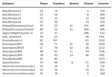
The set of instances available from Third ITC http://www. utwente.nl/ctit/hstt/archives/XHSTT-2012 was originated from many countries and ranges from small instances to huge challen-ging ones.Table 1presents the main features of these problems.

4.2. Obtained results

In the first set of experiments we evaluated the proposed methods using the same metric employed in the Third ITC : average results produced in a restricted time limit, as discussed in the beginning of this section. Table 2 presents the obtained average results of the basic VNS method (BVNS) and its variations: RVNS, SVND and SVNS. We also included in this table the results of the KHE engine[30]initial solutions as well as the results of the Third ITC winner, a Simulated Annealing-Iterated Local Search approach[9]. These results are presented in columns KHE and SA-ILS. Each cell includes the average result of five independent executions3_{of one method on a given instance.}

Table 3 presents the ordering of the presented methods according to the Third ITC rules. Each solver receives a rank in each instance ranging from 1 (best) to 4 (worst) according to the average costs of solutions obtained. The solver with the smaller average rank is considered the best.

Brito et al.[31]presented another VNS based approach to this problem. In their work, they used the Simulated Annealing algorithm to perform the local search at each iteration of VNS. They used the public set of instances from ITC to evaluate their approach since the hidden set was not released yet.

Table 4 presents the comparison between the SVNS method and the results presented by Brito et al.[31]. The best result on each instance is highlighted in bold.

4.3. Discussion of results

For some instances, even the production of feasible solutions configures a hard task. These instances commonly define most constraints as hard constraints. The VNS approach and its varia-tions were able to find 12 out of 18 feasible solutions to the instance set, one more than the Third ITC winner.

As it can be seen inTable 2, the VNS based approach was able to outperform the Third ITC winner. More specifically, the SVNS algo-rithm presented better results in most of the instances. One explana-tion to this result may be the fact that SVNS has an improved mechanism to escape from large valleys which does not rely only on randomness.

To understand the positive effect of the controlled diversifi ca-tion in SVNS we plotted in Fig. 1 the evolution in time of the relative distance (gap) of the cost of the incumbent solution to the best known solution in BVNS and SVNS for two hard instances. Considering the incumbent solution costcand the best known solution cost cn

the gap is computed at each time instant as

ðc cn

Þ=cn

. The cost is a fixed point value where the integer part corresponds to the feasibility cost and the fractional part to the quality cost. As it can be seen inFig. 1, while in the beginning of the search both methods are comparable, SVNS improves solutions much more often as the search process advances.

The algorithm RVNS presented a poor performance. We believe that the fact that it does not systematically reach different local optima contributed to these poor results. Moreover, an excessive exploration in larger, more expensive neighborhoods, may also slow down the search in cases where improvement movements could be found in smaller neighborhoods.

We compared the method which found the best results, SVNS, to the SA-VNS approach presented by Brito et al.[31]. SVNS was able to outperform the SA-VNS results in 14 out of 19 instances. This result points that a descent method may be more effective than the Simulated Annealing method to perform local search at each iteration of VNS for this problem. The RNA descent method which we implemented has a smaller computational cost and has only one parameter to tune. Note that SA-VNS performed better than SVNS in the easy instances, since the computational cost of Simulated Annealing is not a problem in these cases.

5. Concluding remarks

The VNS algorithm showed strong results when applied to the High School Timetabling Problem, outperforming the Third ITC

Table 1

Features of considered instances from Third ITC.

Instance Times Teachers Rooms Classes Lessons

BrazilInstance2 25 14 6 150

BrazilInstance3 25 16 8 200

BrazilInstance4 25 23 12 300

BrazilInstance6 25 30 14 350

FinlandElementarySchool 35 22 21 291 445

FinlandSecondarySchool2 40 22 21 469 566

Aigio1stHighSchool10-11 35 37 208 532

Italy_Instance4 36 61 38 1101

KosovaInstance1 62 101 63 1912

Kottenpark2003 38 75 41 18 1203

Kottenpark2005A 37 78 42 26 1272

Kottenpark2008 40 81 11 34 1118

Kottenpark2009 38 93 53 48 1301

Woodlands2009 42 40 1353

Spanishschool 35 66 4 21 439

WesternGreeceUniversity3 35 19 6 210

WesternGreeceUniversity4 35 19 12 262

WesternGreeceUniversity5 35 18 6 184

2_{The CPU time was adjusted in our computer using the ITC benchmark} software, which suggested 1500 s.

3

winner approach. This result coupled with another recent reports in literature[25–27,32]points that VNS and its variations are very

good alternatives for the heuristic solution of timetabling and scheduling problems.

Contrary to the tradition established by the last three timetabl-ing competitions, where the best timetabltimetabl-ing solvers incorporated

Table 2

Average results produced with VNS variants and other approaches in the restricted time limit of the Third ITC.

Instance KHE[30] SA-ILS[9] BVNS RVNS SVND SVNS

BrazilInstance2 4/90 1.0/63.9 0.0/40.6 2.2/71.4 0.6/63.8 0.0/39.6

BrazilInstance3 3/240 0.0/127.8 0.0/113.0 2.4/151.4 1.6/136.8 0.0/119.0

BrazilInstance4 39/144 17.2/99.6 4.8/108.2 21.0/112.8 13.6/103.4 3.8/123.4

BrazilInstance6 11/291 4.0/223.5 0.0/157.4 6.0/271.0 2.2/231.2 0.0/151.4

FinlandElementarySchool 9/30 0.0/4.0 0.0/3.4 2.6/7.4 0.0/4.0 0.0/3.8

FinlandSecondarySchool2 2/1821 0.0/0.4 0.0/0.4 0.6/86.8 0.0/1.0 0.0/0.4

Aigio1stHighSchool10-11 14/757 0.0/15.3 0.4/10.2 11.2/200.0 4.8/259.0 0.2/8.2

ItalyInstance4 39/21,238 0.0/658.4 0.0/409.0 0.4/2666.6 0.0/1271.0 0.0/324.8

KosovaInstance1 1333/566 14.0/6934.4 1.2/20.4 31.6/278.8 2.0/75.6 1.2/17.4

Kottenpark2003 3/78,440 0.6/90,195.8 2.0/10,217.2 2.4/34,766.0 2.8/7937.8 2.0/9694.4

Kottenpark2005A 35/23,677 33.9/27,480.4 33.8/19,059.2 35.0/22,914.0 27.0/10,118.0 33.8/18,547.6

Kottenpark2008 63/140,083 25.7/31,403.7 15.6/23,962.0 36.8/38,936.6 16.8/33,443.6 15.8/24,024.2

Kottenpark2009 55/211,095 36.6/15,4998.5 35.0/8543.0 45.4/148,601.0 31.2/8563.0 33.2/9667.0

Woodlands2009 19/0 2.0/15.8 2.0/8.2 10.8/16.4 2.0/14.4 2.0/6.2

Spanish school 1/4103 0.0/865.2 0.0/907.8 0.0/3068.0 0.0/1126.0 0.0/724.2

WesternGreeceUniversity3 0/30 0.0/5.6 0.0/5.4 0.0/20.4 0.0/15.2 0.0/5.0

WesternGreeceUniversity4 0/41 0.0/7.4 0.0/6.4 0.0/30.0 0.0/23.6 0.0/5.6

WesternGreeceUniversity5 17/44 0.0/0.0 0.0/0.0 2.8/16.2 1.2/3.0 0.0/0.0

Average 91.5/26,816.11 7.5/17,394.4 5.3/3531.8 11.7/14,011.9 5.9/3521.7 5.1/3525.7

Table 3 Solvers ranking.

Instance SA-ILS[9] BVNS RVNS SVND SVNS

BrazilInstance2 4.0 2.0 5.0 3.0 1.0

BrazilInstance3 3.0 1.0 5.0 4.0 2.0

BrazilInstance4 4.0 2.0 5.0 3.0 1.0

BrazilInstance6 4.0 2.0 5.0 3.0 1.0

FinlandElementarySchool 3.5 1.0 5.0 3.5 2.0

FinlandSecondarySchool2 2.0 2.0 5.0 4.0 2.0

Aigio 1st High School 2010-2011 1.0 3.0 5.0 4.0 2.0

Italy_Instance4 3.0 2.0 5.0 4.0 1.0

KosovaInstance1 4.0 2.0 5.0 3.0 1.0

Kottenpark2003 1.0 3.0 4.0 5.0 2.0

Kottenpark2005A 4.0 3.0 5.0 1.0 2.0

Kottenpark2008 4.0 1.0 5.0 3.0 2.0

Kottenpark2009 4.0 3.0 5.0 1.0 2.0

Woodlands2009 4.0 2.0 5.0 3.0 1.0

Spanish school 2.0 3.0 5.0 4.0 1.0

WesternGreeceUniversityInstance3 3.0 2.0 5.0 4.0 1.0 WesternGreeceUniversityInstance4 3.0 2.0 5.0 4.0 1.0 WesternGreeceUniversityInstance5 2.0 5.0 4.0 2.0 2.0

Average 3.08 2.28 4.89 3.25 1.50

Table 4

Comparative between SA-VNS approach[31]and SVNS approach.

Instance SA-VNS[31] SA-RVNS[31] SVNS

AustraliaBGHS98 11/475 11/475 9/411

AustraliaSAHS96 18/52 18/52 19/30

AustraliaTES99 9/187 9/187 9/177

BrazilInstance1 0/21 0/44 0/17

BrazilInstance4 12/123 12/153 1/90

BrazilInstance5 4/148 4/184 0/78

BrazilInstance6 4/213 4/213 0/151

BrazilInstance7 11/267 11/318 0/242

EnglandStPaul 2/48,758 2/48,450 1/26,258 FinlandArtificialSchool 19/12 19/12 6/5

FinlandCollege 1/49 1/77 2/32

FinlandHighSchool 0/16 0/73 0/29

FinlandSecondarySchool 0/114 0/129 1/94

GreecePatras3rdHS2010 0/12 0/20 0/0

GreecePreveza3rdHS2008 0/37 0/33 0/4

ItalyInstance1 0/20 0/31 0/24

Kottenpark2003 1/72,413 0/85,372 0/9365

Kottenpark2005 20/28,710 20/28,482 18/10,052

SouthAfricaLewitt2009 0/78 0/74 0/8

0 0.05 0.1 0.15 0.2 0.25 0.3 0.35 0.4 0.45 0.5

0 200 400 600 800 1000 1200 1400

average gap (%)

time (sec) SpainSchool

BVNS SVNS

0 0.2 0.4 0.6 0.8 1

0 200 400 600 800 1000 1200 1400

average gap (%)

time (sec) Kottenpark2003

BVNS SVNS

Simulated Annealing in some form, we demonstrated that a proper implementation of the Skewed VNS method provides an excellent heuristic for the High School Timetabling Problem. We consider that the VNS approach has two important advantages when compared to SA based approaches: VNS usually has less parameters to tune and these parameters are not sensible to scales.

Some possible future works are to (1) implement and evaluate another metaheuristics to this problem, like evolutionary algorithms; (2) implement other neighborhood movements; and (3) develop a graphical user interface and allow schools and universities from all around the world to produce their instances and solve them with our solver.

References

[1]Even S, Itai A, Shamir A. On the complexity of timetable and multicommodity flow problems. SIAM J Comput 1976;5(4):691–703.

[2]Garey MR, Jonhson DS. Computers and intractability: a guide to the theory of NP-completeness. San Francisco, CA, USA: Freeman; 1979.

[3] IDSIA. International Timetabling Competition 2002. Available at〈http://www. idsia.ch/Files/ttcomp2002/〉; 2012 [accessed December 2012].

[4] Kostuch P. The university course timetabling problem with a three-phase approach. In: Proceedings of the 5th international conference on practice and theory of automated timetabling. Berlin, Heidelberg: Springer-Verlag; 2005. p. 109–25.

[5]Kirkpatrick S, Gellat DC, Vecchi MP. Optimization by simulated annealing. Science 1983;202:671–80.

[6] McCollum B. International Timetabling Competition 2007. Available at〈http:// www.cs.qub.ac.uk/itc2007/〉; 2013 [accessed December 2012].

[7] Müller T. ITC2007 solver description: a hybrid approach. Ann Oper Res 2009;172:429–46.

[8] University of Twente. International Timetabling Competition 2012. Available at 〈http://www.utwente.nl/ctit/hstt/itc2011/welcome/〉; 2012 [accessed December 2012].

[9] Fonseca G, Santos H, Toffolo T, Brito S, Souza M. GOAL solver: a hybrid local search based solver for high school timetabling. Ann Oper Res 2014 [in press].

[10]Santos HG, Uchoa E, Ochi LS, Maculan N. Strong bounds with cut and column generation for class-teacher timetabling. Ann Oper Res 2012;194:399–412. [11]Daskalaki S, Birbas T, Housos E. An integer programming formulation for a

case study in university timetabling. Eur J Oper Res 2004;153(1):117–35. [12]Tripathy A. School timetabling—a case in large binary integer linear

program-ming. Manag Sci 1984;30(12):1473–89.

[13] Haspeslagh S, De Causmaecker P, Stolevik M, Schaerf A. First international nurse rostering competition 2010. Technical report, CODeS. Belgium: Depart-ment of Computer Science, KULeuven Campus Kortrijk; 2010.

[14] Post G, Ahmadi S, Daskalaki S, Kyngas J, Nurmi C, Ranson D, et al. An XML format for Benchmarks in High School Timetabling. In: PATAT'08 Proceedings

of the 7th international conference on the practice and theory of automated timetabling, vol. 03018, 2008.

[15] Post, Gerhard, Kingston, Jeffrey H, Ahmadi, Samad, Daskalaki, Sophia, Gogos, Christos, Kyngas, Jari, Nurmi, Cimmo, Musliu, Nysret, Pillay, Nelishia, Santos, Haroldo, Schaerf, Andrea. XHSTT: an XML archive for high school timetabling problems in different countries. Ann. Oper. Res. 2011;1–7./http://dx.doi.org/ 10.1007/s10479-011-1012-2S.

[16] Kingston JH. A tiling algorithm for high school timetabling. Lecture notes in computer science: V practice and theory of automated timetabling, vol. 3616. Berlin: Springer; 2005. p. 208–25.

[17]Wright M. School timetabling using heuristic search. J Oper Res Soc 1996;47: 347–357.

[18] Nurmi K, Kyngas J. A framework for school timetabling problem. In: Proceed-ings of the 3rd multidisciplinary international scheduling conference: theory and applications, Paris, 2007. p. 386–93.

[19]Valourix C, Housos E. Constraint programming approach for school time-tabling. Comput Oper Res 2003;30:1555–72.

[20] de Haan P, Landman R, Post G, Ruizenaar H. A case study for timetabling in a Dutch secondary school. Lecture notes in computer science: VI practice and theory of automated timetabling, vol. 3867. Berlin: Springer; 2007. p. 267–79.

[21] Post, Gerhard, Ahmadi, Samad, Daskalaki, Sophia, Kingston, Jeffrey H, Kyngas, Jari, Nurmi, Cimmo, Ranson, David. An XML format for benchmarks in high school Timetabling. Ann. Oper. Res. 2012;194(1):385–397. /http://dx.doi.org/10.1007/ s10479-010-0699-9S.

[22] Kingston JH. A software library for school timetabling. Available at〈http:// sydney.edu.au/engineering/it/jeff/khe/〉; May 2012.

[23] Kingston JH. Hierarchical timetable construction. In: Problems, proceedings of thefirst international conference on the practice and theory of automated timetabling, 2006.

[24] Mladenovic N, Hansen P. Variable neighborhood search. Comput Oper Res 1997;24:1097–100.

[25]Costa WE, Goldbarg MC, Goldbarg EFG. New VNS heuristic for totalflowtime flowshop scheduling problem. Expert Syst Appl 2012;39:8149–61. [26]Vlah S, Lukac Z, Pacheco J. Use of VNS heuristics for scheduling of patients in

hospital. J Oper Res Soc 2011;62:1227–38.

[27] Wang X, Tang L. A Hybrid VNS with TS for the single machine scheduling problem to minimize the sum of weighted tardiness of jobs. In: Proceedings of the 4th international conference on intelligent computing: advanced intelli-gent computing theories and applications–with aspects of artificial

intelli-gence. Berlin, Heidelberg: Springer-Verlag; 2008. p. 727–33.

[28] Hansen P, Mladenović N. Variable neighborhood search: principles and applications. Eur J Oper Res 2001;130:449–67.

[29] Hansen P, MladenovićN. Variable neighborhood search: a chapter of hand-book of applied optimization. Les Cahiers du GERAD G-2000-3. Montreal, Canada, 2000 (Chapter 8).

[30] Kingston JH. A software library for school timetabling. Available at〈http:// sydney.edu.au/engineering/it/jeff/khe/〉; 2012 [accessed December 2012]. [31]Brito SS, Fonseca GH, Toffolo TA, Santos HG, Souza MJ. A SA-VNS approach for

the high school timetabling problem. Electron Notes Discr Math 2012;39: 169–176.