Stochastic Measurement Models for
Quantifying Lymphocyte Responses Using
Flow Cytometry
Andrey Kan1,2, Damian Pavlyshyn1,2¤a, John F. Markham1,2¤b, Mark R. Dowling1,2,
Susanne Heinzel1,2, Jie H. S. Zhou1,2, Julia M. Marchingo1,2, Philip D. Hodgkin1,2*
1Division of Immunology, The Walter and Eliza Hall Institute of Medical Research, Parkville, VIC, Australia, 2Department of Medical Biology, The University of Melbourne, Parkville, VIC, Australia
¤a Current Address: Department of Mathematics and Statistics, The University of Melbourne, Parkville, VIC, Australia
¤b Current Address: Cancer Research Division, Peter MacCallum Cancer Centre, East Melbourne, VIC, Australia
Abstract
Adaptive immune responses are complex dynamic processes whereby B and T cells undergo division and differentiation triggered by pathogenic stimuli. Deregulation of the response can lead to severe consequences for the host organism ranging from immune deficiencies to autoimmunity. Tracking cell division and differentiation by flow cytometry using fluorescent probes is a major method for measuring progression of lymphocyte responses, both in vitro and in vivo. In turn, mathematical modeling of cell numbers derived from such measurements has led to significant biological discoveries, and plays an increas-ingly important role in lymphocyte research. Fitting an appropriate parameterized model to such data is the goal of these studies but significant challenges are presented by the vari-ability in measurements. This variation results from the sum of experimental noise and intrinsic probabilistic differences in cells and is difficult to characterize analytically. Current model fitting methods adopt different simplifying assumptions to describe the distribution of such measurements and these assumptions have not been tested directly. To help inform the choice and application of appropriate methods of model fitting to such data we studied the errors associated with flow cytometry measurements from a wide variety of experi-ments. We found that the mean and variance of the noise were related by a power law with an exponent between 1.3 and 1.8 for different datasets. This violated the assumptions inherent to commonly used least squares, linear variance scaling and log-transformation based methods. As a result of these findings we propose a new measurement model that we justify both theoretically, from the maximum entropy standpoint, and empirically using collected data. Our evaluation suggests that the new model can be reliably used for model fitting across a variety of conditions. Our work provides a foundation for modeling measure-ments in flow cytometry experimeasure-ments thus facilitating progress in quantitative studies of lym-phocyte responses.
OPEN ACCESS
Citation:Kan A, Pavlyshyn D, Markham JF, Dowling MR, Heinzel S, Zhou JHS, et al. (2016) Stochastic Measurement Models for Quantifying Lymphocyte Responses Using Flow Cytometry. PLoS ONE 11(1): e0146227. doi:10.1371/journal.pone.0146227
Editor:Andrew J. Yates, University of Glasgow, UNITED KINGDOM
Received:July 14, 2015
Accepted:November 9, 2015
Published:January 7, 2016
Copyright:© 2016 Kan et al. This is an open access article distributed under the terms of theCreative Commons Attribution License, which permits unrestricted use, distribution, and reproduction in any medium, provided the original author and source are credited.
Data Availability Statement:All relevant data are within the paper and its Supporting Information files.
https://education.gov.au/australian-Introduction
In response to pathogenic stimuli, B and T lymphocytes undergo proliferation and differentia-tion into effector and memory cells. Dysreguladifferentia-tion at any stage of this process can lead to severe consequences for the host organism, ranging from autoimmune diseases and transplant rejection to immunodeficiency and cancer. Obtaining a quantitative understanding of lympho-cyte response regulation poses a significant theoretical and practical challenge for modern immunology. It is increasingly evident that the study of such a complex biological phenome-non will require an interdisciplinary approach. Indeed, mathematical modeling of proliferating
lymphocytes has played a central role in a number of major biological discoveries [1–3].
More-over, a quantitative study of the effects of different signals on proliferation and survival param-eters has enabled accurate prediction of lymphocyte expansion kinetics in response to signal modulation [4]. Such predictive power can be employed in next generation drug screening platforms for a range of therapies, including cancer immunotherapy [5].
Flow cytometry using a wide array of fluorescence probes is one of the most powerful
meth-ods used to measure the progression of lymphocyte responses bothin vivoandin vitro[6]. It is
therefore not surprising that an increasing number of research groups fit and validate their
mathematical models of lymphocyte responses against flow cytometry data [4,7–13]. Division
tracking dyes, such as carboxyfluorescein succinimidyl ester (CFSE) or CellTrace Violet (CTV), enable estimation of the number of cells that have undergone a certain number of
divi-sions after activation [14,15]. These data alone have been instrumental for developing models
of lymphocyte proliferation, such as systems of ordinary differential equations [16], branching process-based formulations [17], or the Cyton model [18].
Moreover, the range of fluorescent probes is not restricted to division tracking (Fig 1). For example, the Blimp1-green fluorescent protein (GFP) reporter mouse is useful for quantifying B cell differentiation into plasma cells [19], and the fluorescent ubiquitination-based cell-cycle indicator (FUCCI) system is a powerful tool for measuring cell cycle progression [20]. These and other types of measurements support the development of mathematical models for various aspects of lymphocyte responses. Here, we consider flow cytometry measurements, obtained using division tracking dyes, or other probes, and the accordingly suitable mathematical mod-els used to fit these data, collectively calledresponse models. We note that flow cytometry data is expected to remain a major source of information for the response models in future due to the growing arsenal of fluorescent probes, their applicabilityin vivo, and their broad applicabil-ity in many biological contexts.
There is considerable variation in measurements repeated for the same time point and experimental conditions. This variation arises from two sources. First, biological variation arises due to inherent cell-to-cell variability. For example, even sister cells can have different division times or different fates where one cell dies and another cell divides [21]. Second, exper-imental error denotes collective variations contributed by different steps of the experexper-imental procedure. Experimental error is responsible for the bulk of variation in measurements [22], and therefore cannot be ignored during model fitting. While biological variation can be explic-itly characterized as a part of a lymphocyte proliferation model [13,22], it is extremely difficult to formalize experimental error. This variability originates from pipetting errors, variation in number of cells processed by a flow cytometer (sample recovery), and multi-level semi-manual gating. Note that raw flow cytometry measurements are inevitably subject to at least two rounds of gating, whereby a researcher first separates live cells from calibration beads and dead cells [23], and then applies a gate on a particular fluorescent probe (Fig 1). In some experi-ments, an additional round of gating is needed to isolate the cell population of interest (e.g., where transgenic cells were adoptively transferred). In practice, all these gates are either drawn postgraduate-awards). J.M.M. was the recipient of an
Australian Postgraduate Award, WEHI Edith Moffat Scholarship and Sydney Parker Smith Postdoctoral Research Fellowship from the Cancer Council of Victoria ( https://education.gov.au/australian-postgraduate-awards). The funders had no role in study design, data collection and analysis, decision to publish, or preparation of the manuscript.
entirely manually, or set automatically, but then adjusted manually. As such, experimental error is one of the major challenges of model fitting.
The difficulty in finding an explicit experimental error characterization has lead to an approach where all the stochastic biological and experimental effects are attributed to a single process (Fig 2) which is formalized using some assumed probability distribution for
measure-ments [10,11,13]. This measurement distribution can then be used for model fitting, e.g.,
assuming normality of measurements with fixed variance leads to least-squares fitting. The problem is that different researchers have been using different sets of assumptions for fitting to
the same type of data [10,11,13]. Moreover, within the same work one set of assumptions
(e.g., measurement variance scaling with the mean) can be adopted for parameter estimation, while another set of assumptions (e.g., constant variance) is used for model selection using
information-theoretic criteria [11,24].Here we study the distribution of measurements from
representative experiments as an important step towards adoption of a single standard method
for estimating parameters from flow cytometry data.
Fig 1. Measuring lymphocyte responses using a range of fluorescent probes.Panels show flow cytometry results for a time point from different representative B or T cell activation experiments. A: CTV can be used to estimate number of cells that divided 4 times since activation (“generation 4”gate). B: Blimp1-GFP reporter and IgG1-APC antibody enable estimation of non-differentiated cells (purple gate). IgG1-APC is a fluorescent probe-conjugated antibody against IgG. C: FUCCI reporter system allows one to estimate cells in different cell cycle stages (labeled quadrants). In each case, estimates are obtained using semi-manual gates. Such gates can be initially set using an automated routine, but it is a common practice to manually validate and adjust the gates.
doi:10.1371/journal.pone.0146227.g001
Fig 2. Measurement process encapsulates biological variability and experimental error.Since it is difficult to formalize experimental error, a common strategy is to consider a stochastic measurement generating process as a whole. Measurements can then be described using a measurement distribution. Internally, this distribution is a result of stochastic lymphocyte response and experimental error (including data pre-processing, such as gating).
To this end, we explore lymphocyte response data (both new and previously published) from a wide range of experimental conditions focusing on immunological applications. Based on these data, we develop a new measurement model and corresponding model fitting method. In addition to the data, we provide a theoretical support for our model from a maximum entropy standpoint. Our evaluation shows that the new method can be reliably used for model fitting across a variety of conditions, thus providing a foundation for model development in the field of quantitative lymphocyte research.
Related Work
There has been a large number of proposed lymphocyte response models, as well as parameter
estimation strategies for flow cytometry data [4,7–13]. In this work, we focus on parameter
estimation strategies and the assumptions involved in these strategies. These strategies can be broadly categorized in heuristic and probabilistic approaches. In a heuristic approach, a
lym-phocyte response model is used to predict expected values of measurements, and anad hoc
function is defined to characterize the discrepancy between the predictions and the data [12,
13,24]. This discrepancy is then minimized as a function of response model parameters.
Prob-abilistic approaches, on the other hand, attempt to define the probability of the measured data
given response model parameters [10,13]. This probability can then be used in different ways,
for example, in maximum likelihood (ML) or Bayesian parameter estimation algorithms. It is important to acknowledge that various assumptions can be heuristically adopted in order to derive the probability of measurements. However, the probabilistic approach still has the advantage that all assumptions can be explicitly identified and tested.
A measurement can be viewed as the sum of two random variables corresponding to lym-phocyte response and experimental error (Fig 2). In most lymlym-phocyte response models, the population response is considered as the sum of independent single cell responses, and the cen-tral limit theorem can be used to argue that the response outcomes are approximately normal. It is then possible to explicitly model experimental error in the context of CFSE experiments by
describing the process of peak generation on a CFSE histogram [12,25]. However, such an
approach does not take into account other steps of experimental procedure, including live cell gating, and also is not applicable to other types of flow cytometry experiments, such as those involving Blimp1-GFP or FUCCI reporters. Alternatively, other probabilistic methods assume
a certain probability distribution directly for measurements [10,11,13,24]. It is also assumed
that expected values of the response model (as a function of model parameters) are indicative
of the expected values of the measurements [11,13,24]. Next, many methods adopt the
simpli-fying assumption that the measurement covariance matrix is diagonal [10,11,24].
Probabilistic measurement models are used for both parameter estimation and model selec-tion based on informaselec-tion criteria, such as corrected Akaike Informaselec-tion Criterion (AICc), and Bayesian Information Criterion (BIC). These criteria require an estimate of the probability of the data [26], i.e., a probabilistic measurement model. For such a model, some authors adopt
a multivariate normal distribution with a constant variance [11,24], while others assume
con-stant marginal variances of log-transformed data [10]. These previous measurement models are formally described inS1 Text. A point of concern here is that in some cases, fitting is per-formed using a different criterion than the one used for model selection. For example, for the purposes of fitting, marginal variances can be assumed to scale linearly with the expected val-ues, while for the purposes of model selection these variances can be assumed to be constant
[24]. Here, we aim to test the above assumptions (summarized inTable 1) against a large
facilitate the development of a single measurement model that can be reliably used for both fit-ting and model selection across a wide range of lymphocyte studies.
Having introduced the prior art, we can now elaborate on the question that we address in this work. Given data and a set of predicted mean cell counts produced by a response model (e.g., Cyton or multitype branching process), we ask which objective function one should use
for parameter estimation. Different previous models listed inTable 1will lead to different
objective functions (in this case, likelihoods). As we show in subsequent sections, the assump-tions behind some of these likelihood funcassump-tions are inconsistent with the data, and the choice of the function makes a difference to the final solution. Next, we present a new measurement model and the corresponding likelihood function. Finally, note that different likelihoods, including the likelihood derived from our model, can be used in situations where single or mul-tiple parameter sets that maximize the likelihood are explored (search for global and local max-ima, respectively).
Results
We start with outlining the notation principles used in this paper. We use lowercase symbols to denote constant scalar values (e.g.,x,σ) which can be vector or matrix components (e.g.,xi,σij),
symbols in boldface to denote constant vectors and matrices (e.g.,x,S), uppercase symbols to
denote random variables (e.g.,X,Δ), and blackboard bold symbols for sets (e.g.,D). For multi-variate random variables, indexing can be used to denote a marginal variable (e.g.,Xi,Δj). Fur-thermore, sample parameter estimates are denoted using a hat (e.g.,^x;^μ). Finally,R
pdenotesp
−dimensional Euclidean space, andRpþdenotes a non-negative Euclidean subspace, i.e., for ap
−dimensional vector,x2Rpþmeans thatxi0,i= 1,. . .,p.
Experimental data
A dataset is a set of samplesD¼ fT
ð1Þ;. . .;TðdÞg, where each sampleTðtÞ ¼ fzðt
;1Þ;
. . .;zðt
;stÞgis
a set ofstrepeated measurements (replicates) taken at a distinct time point. We assume that all
measurements from the same time point are generated by the same distribution that character-izes the lymphocyte response at that time point. Samples from different time points may come from different distributions. Each measurementz(t,r)is ap-dimensional vector, where compo-nentz(t,r),idenotes the estimated number of cells that belong to groupi. Examples of groups include cells that have divided two times since the beginning of the experiment, cells that have differentiated, or cells that have returned to quiescence. Different experiments can measure
dif-ferent quantities and result in datasets covering difdif-ferent groups. A range offluorescent probes
and semi-manual gating are used to assign cells to groups. Note thatz(t,r),icannot be negative,
Table 1. Assumptions involved in previous measurement models (used either for model fitting or model selection).
Approach Assumptions Ref.
sum of squared residuals (SSR) multivariate normal (MVN) distribution of measurements; diagonal covariance matrix; same marginal variances for all dimensions and time points
[11]
log-transformed sum of squared residuals (LogNrm)
multivariate lognormal distribution of measurements; diagonal covariance matrix for log-transformed data; same marginal variances for log-transformed samples
[10]
linear variance scaling (LVS) MVN distribution of measurements; diagonal covariance matrix; linear relationship between marginal variances and means
[24]
but can be a fraction, because the estimation involves normalization using calibration bead counts [27].
Consider a lymphocyte response model with parameter vectorθ(e.g., Cyton model with
parameters such as mean time to first division, mean division destiny, etc. [18]; or a branching process with probabilities of division, death, etc. [7,11,13]). A probabilistic parameter estima-tion approach first aims to define the likelihoodLðθjDÞ ProbðDjθÞ. The experiments can be
performedin vitroorin vivo. Here we focus on widely used protocols where repeated
observa-tions are measured from distinct physically separated wellsin vitroor from different animalsin
vivo[4,24]. Therefore, it is reasonable to assume independence, conditioned on a model with
fixed parameter values, not only for different time points, but also for observations (i.e.,
repli-cates) within the same time point. More discussion on this assumption is provided inS2 Text.
That is, we assume that (a) observations for different time points are independent: PrðT
ðiÞ;TðjÞjθÞ ¼PrðTðiÞjθÞPrðTðjÞjθÞ,i6¼j, and (b) the repeated observationsz(t,r)for a given time pointtare independent and identically distributed (i.i.d.). Therefore, ifZ(t)denotes the measurement random variable (that incorporates both biological variation and experimental noise), we can write
LðθjDÞ ¼Y
d
t¼1
Y
st
r¼1
PðZðtÞ¼zðt;rÞjθÞ
!
ð1Þ
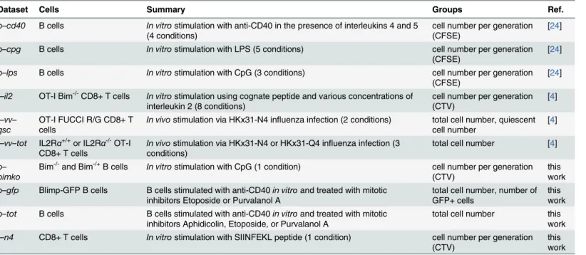
In order to explore the properties of distribution ofZ(t)in real world situations, we collect data from a number of independent experiments (either from published sources or executed for this study). We aim to collect data that represent a large variety of conditions encountered in lymphocyte studies (Table 2), and cover a range of cell types (wild type B or T cells, as well
as knock outs), stimulation protocols, and treatmentsin vitroandin vivo. Importantly, the
def-inition of a group (i.e., what is being measured) varies across experiments. For example,
experi-mentsb–cd40andt–n4represent typical proliferation assays based on the use of CFSE or CTV
dyes. In these, and similar experiments, for each time point,Z(t)is a vector comprising the esti-mated number of cells per generation. In contrast, measurementsZ(t)in datasett–vv–qscare
two-dimensional vectors containing total cell number, as well as the number of cells returned to a quiescent state. Quiescent cells were estimated based on FUCCI expression and cell size. Six datasets were obtained from previous studies, while the remaining four experiments were conducted specifically for this study. These include a proliferation assay with 9 replicates per time point (datasetb–bimko). A typical number of replicates (st) is 3 to 5, and a dataset with a
large number of replicates is useful in studying the distribution of measurements. Finally, we include two experiments where proliferating B cells are treated with mitotic inhibitors (b–gfp
andb–tot). These two datasets cover a combination of drugs, but contain only one time point
for each condition. All data can be found inS1 Dataset.
Mean
–
variance relation
Previous approaches have made specific assumptions about the marginal variances ofZ(t)
(Table 1). Therefore, we first inspect the relation between means and marginal variances for
each vector component for samplesT
ðtÞ ¼ fzðt;1Þ;
. . .;zðt
;stÞg. Our datasets represent a range of
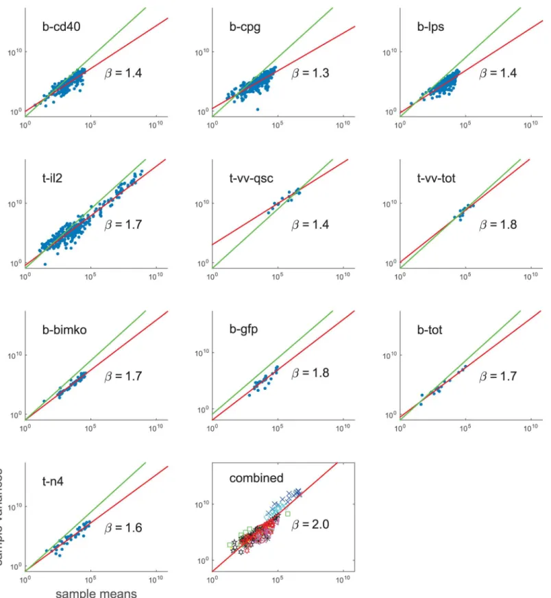
experimental conditions and measured quantities. Strikingly, despite this variety,
measure-ments from all experimeasure-ments tend to follow a power law (Fig 3andS1 Table). Marginal variances
of measurements, as well as log-transformed measurements span several orders of magnitude
and there is a statistically significant correlation with measurement means (S1 FigandS1
violated. Moreover, we estimate the power exponent using a linear regression on a
log-trans-formed axes, andfind that in almost all datasets 95% confidence intervals for the estimated
power exponent do not include 1, which is not consistent with the linear scaling assumption of LVS model. We conclude that the data does not support any of the previously used assumption sets listed inTable 1.
Points inFig 3can represent different quantities, such as the number of cell in a particular
generation, or the number of differentiated cells. It is therefore interesting that all experiments exhibit a similar pattern. For example, residuals after power law fits tend to follow the same dis-tribution across experiments (Kruskal-Wallis test p-value 0.998, number of points ranging from 12 to 321); and in each experiment, residuals tend to be centered around 0 (sign test
p-values above 0.02 for each dataset, seeS1 Table). Consistent with a previous observation [22],
this may indicate that the experimental error originating from sources common to all datasets dominates variation in measurements. Such sources can include pipetting error, sample recov-ery by the flow cytometer, and effects of manual gating. Regardless of whether variability in these data originated mostly from biology or experimental procedure, we make an empirical observation that superficially measurement variance scales with mean according to a power law (that can have a different exponent for different datasets).
Application of the maximum entropy principle
Computing the likelihood of parameters requires specification of the shape of a multivariate
distribution of measurementsZ(t), and an MVN with independent components is a popular
choice [11,24,28]. The literature on computational immunology says little about the
justifica-tion of these assumpjustifica-tions. The central limit theorem can be used to argue for an
MVN-distrib-utedtruecell numbers, but this argument is difficult to apply for measurements that include
various sources of experimental errors. Therefore, we find it useful to present a systematic approach for justifying the choice of measurement distribution in the context of lymphocyte responses.
Table 2. Summary of experimental data used in this work.
Dataset Cells Summary Groups Ref.
b–cd40 B cells In vitrostimulation with anti-CD40 in the presence of interleukins 4 and 5
(4 conditions)
cell number per generation (CFSE)
[24]
b–cpg B cells In vitrostimulation with LPS (5 conditions) cell number per generation
(CFSE)
[24]
b–lps B cells In vitrostimulation with CpG (3 conditions) cell number per generation
(CFSE)
[24]
t–il2 OT-I Bim-/-CD8+ T cells In vitrostimulation using cognate peptide and various concentrations of
interleukin 2 (8 conditions)
cell number per generation (CTV)
[4]
t–vv–
qsc
OT-I FUCCI R/G CD8+ T cells
In vivostimulation via HKx31-N4 influenza infection (2 conditions) total cell number, quiescent
cell number
[4]
t–vv–tot IL2Rα+/+or IL2Rα-/-OT-I
CD8+ T cells
In vivostimulation via HKx31-N4 or HKx31-Q4 influenza infection (3
conditions)
total cell number [4]
b–
bimko
Bim-/-and Bim-/+B cells In vitrostimulation with CpG (1 condition) cell number per generation (CTV)
this work
b–gfp Blimp-GFP B cells B cells stimulated with anti-CD40in vitroand treated with mitotic
inhibitors Etoposide or Purvalanol A
total cell number, number of GFP+ cells
this work
b–tot B cells B cells stimulated with anti-CD40in vitroand treated with mitotic
inhibitors Aphidicolin, Etoposide, or Purvalanol A
total cell number this work
t–n4 CD8+ T cells In vitrostimulation with SIINFEKL peptide (1 condition) cell number per generation
(CTV)
this work
In principle, for each experimental scenario, one could perform a large number of replicates to infer the distribution. However, this approach is not practical, due to a large number of pos-sible scenarios (e.g., those listed inTable 2). Therefore, we start with a theoretical argument
justifying a particular choice of the distributiona priori. Further, we have implemented one
experiment with 9 replicates, and in three other datasets we have samples with 5 or 6 replicates (datasetb–bimkoinTable 2), and we use these data to test thea priorihypothesis.
When the information is incomplete (we do not know the true distribution), but a decision has to be made (we need to compute the likelihood), the safest choice would be to minimize the amount of additional information introduced by the decision. A formalization of this prin-ciple is the well known prinprin-ciple of maximum entropy [29]. Suppose we have a method for
pre-dicting mean and covariance ofZ(t)as a function of model parameters. Since measurements
are non-negative quantities, among all possible probability distributions with the given first and second moment, a truncated multivariate normal (TMVN) distribution has the maximum differential entropy (S2 Text). Thus, according to the principle of maximum entropy, TMVN is a feasible choice for the distribution of measurementsa priori. Interestingly, our data suggests that if measurements follow a TMVN distribution, most of the mass of the underlying MVN is
located inRpþ(inFig 3, means tend to be larger than 3 standard deviations).
Therefore, we adopt multivariate normality as a reasonable approximation for measure-ments. In most practical cases, the number of replicates will not be sufficient for reliable selec-tion of the distribuselec-tion based on data, and this is where the principle of maximum entropy can be useful. In experiments with large numbers of replicates the choice of the distribution can be guided by data. In our data collection, we have only several time points (from different experi-ments) with more than 5 replicates, and we have assessed normality on these data (S3 Text). In most cases, the data was consistent with the proposed MVN distribution, and we therefore decided to use it in all cases for consistency. Future measurement models may depart from this decision by using, for example, mixture models, or selecting the shape of the distribution sepa-rately for each time point.
The principle of maximum entropy is also implemented in Dempster’s covariance selection
method [30]. Reliable estimation of off-diagonal covariance elements ofZ(t)is challenging, given that in typical experiments the number of replicates is smaller than the number of dimensions. We observe that in the situation where marginal variances can be predicted, and
off diagonal elements are unknown, Dempster’s method suggests a diagonal covariance matrix
as the most feasible choice (S2 Text). We conclude that the principle of the maximum entropy provides a systematic way for justifying the shape of the distribution of measurements.
Allowing non-zero means for experimental error
To summarize, given a datasetD, a ML or Bayesian parameter estimation routine can use the
likelihood estimated as follows: (1) for each time point, computeηt(θ) =E[Z(t)|θ], whereθis
the candidate parameter vector; (2) estimate dataset-specific power law parametersαandβ
fromD; (3) estimate marginal variancesυii=αηt(θ)β; and (4) compute likelihoodLðθjDÞ
usingEq 1and using the density of MVN with a diagonal covariance matrix.
Going back to step one, consider a lymphocyte response model that predicts meansμt(θ),
and assume that prediction is perfect, and the experimental error has a zero mean, i.e.,
indicating that sample means tend to be larger than 3 standard deviations. If one assumes a Gaussian shape for the distribution of the measurements, this tendency indicates that most of the distribution mass is located in the positive Euclidean subspace.
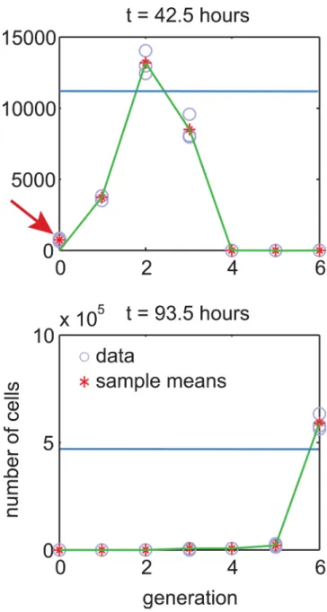
μt(θ) =E[Z(t)|θ]. This assumption can lead to an anomaly illustrated inFig 4. In the figure, the predicted mean is small and so is the predicted variance. Therefore, the likelihood of the green fit is essentially zero, despite the fit visually appearing to be good.
A possible solution to this problem is to assume a minimum measurement variance, i.e., υii=max(c,αηt(θ)β) [24]. However, this approach contradicts the data. For example, dataset t–il2alone has over 10 samples consisting of all zeros (i.e., {0, 0, 0}). All-zero samples are also
Fig 4. The problem of assuming zero mean for experimental error.Consider two fits to the same data extracted fromt–il2dataset for 316 U/mL condition. In this experiment, a data sample comprises repeated
estimates of number of cells in a particular generation. The green fit goes through all generation means, except for the first sample pointed by the arrow. The blue fit predicts an arbitrary value everywhere. Intuitively, the green fit is more feasible, but the blue fit is more likely. This happens because for the first sample variance is close to zero which makes the whole green fit nearly impossible. In practice, mismatch at the first sample can be attributed to a non-zero mean of modeling or experimental noise.
observed in other datasets, which suggests that when the real number of cells is close to 0, so is
the measurement variance. Instead, we note that the real reason, the green fit inFig 4can be
considered feasible, is understanding that (a) a response model is never a perfect representation of reality, and (b) the mean of experimental error can be non-zero. In other words, there can be a difference between the mean of the measurement distribution, and the predicted mean of the
response model. We call this differencemeasurement offset, and propose to model
measure-ment means asηt(θ) =μt(θ)+δ, whereδrepresents the offset. This offset can be estimated from the data, but needs specification of a prior distribution (otherwise an arbitrary fit can be
con-sidered a good fit with a large offset). We developed a maximuma posteriori(MAP) parameter
estimation method, where user needs to specify a reasonable variance onδ(S2 Text). This is
the only user-provided input (denotedε) in the our parameter estimation routine, and the
choice ofεis guided by data. We call our measurement model a three factor (3F) model,
because it accounts for the lymphocyte response model, modeling error, and experimental error (S2 Text).
Evaluation of measurement models
Our ultimate aim is to fit a response model to experimental data. To this end, we take a proba-bilistic approach where a response model is embedded within a measurement model (Fig 2), and focus on different choices for the measurement model. In this section, we assess the perfor-mance of the 3F model and its applicability to fitting. Note that in principle, our conclusions
are not restricted to any particularresponsemodel. For this evaluation, two previous models
were chosen as representative examples, namely Age Dependent Multitype Branching Process (ADMBP) as summarized in reference [11], and the Cyton model as defined in reference [4]. Both models predict the number of cells per generation over time. The Cyton model with 12 parameters is more elaborated than the ADMBP model with 11 parameters. However, note that here we do not aim to compare proliferation models.
In regards to measurement models, we consider those listed inTable 1. For the purposes of
evaluation, it is tempting to generate synthetic data with known response parameters, and assess how these parameters are recovered by different measurement models. However, it is not clear how to generate realistic measurement noise on synthetic data in the first place, since using any of known measurement models, would make the evaluation in favor of that model. Instead, we assess model performance using AICc, and also discuss some theoretical aspects of fitting using different measurement models. In addition, we present a quantitative evaluation using a hypothetical ideal response model. For a given dataset, the hypothetical model simply yields predictions equal to sample means from that dataset. In other words, the hypothetical model mimics the behavior of some accurate model, because an accurate model would be expected to predict values close to the sample means. By the way it is defined it will always out-perform any actual model, such as Cyton or ADMBP in terms of the likelihood of resulting fits.
In terms of the AICc, the“number of parameters”for the hypothetical model is controlled
artificially.
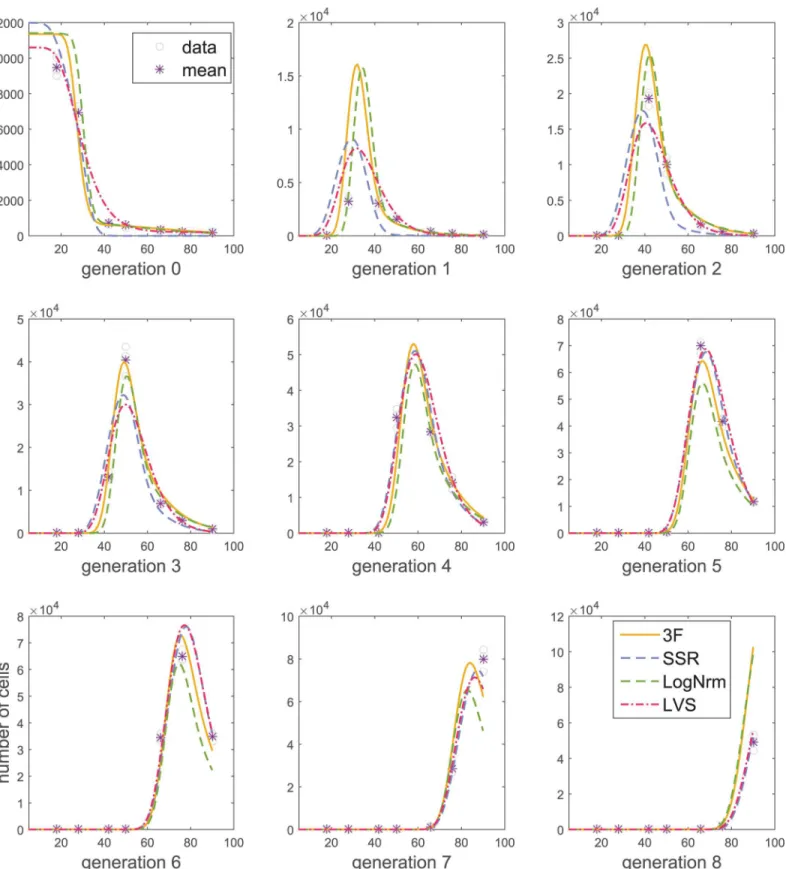
Fig 5. Model fitting using different measurement models.The Cyton model was fitted tot–n4data using different measurement models. Resulting AICc
scores are 2050.7 (3F), 3633.8 (SSR), 4001.7 (LogNrm), and 109231.8 (LVS). For the fit obtained using LogNrm model, AICc was computed using the SSR measurement model.
Next, we note two theoretical inconveniences of the LogNrm model. First, this model assumes that response predictions, such as those produced by ADMBP or Cyton models are medians of measurements, whereas most proliferation models predict the means of the
mea-surements [4,11]. A more severe inconvenience stems from the need of data capping for
log-transformation (S1 Text). Information criteria, such as AICc and BIC cannot be used to com-pare fits performed on capped and original data, or data capped at different levels. Therefore, in this section, for fits obtained using LogNrm model, we report the AICc computed using a SSR model.
Further, for measurement means close to zero (e.g., 0.001), LVS and SSR models allow posi-tive variances (e.g., 10), thus predicting an approximately 50% probability of a negaposi-tive mea-surement. This formulation contradicts the data, and can be one of the reasons for reduced likelihood, compared to the 3F model (Fig 5). Moreover, fits using SSR treat all measurements as equally important (having equal variance), which can lead to undesirable situations where a model cannot predict values close to measurement means for all time points simultaneously. This can be a confounding factor especially for multiconcentration fitting. A
multiconcentra-tion fitting is an emerging problem [4,24], where an experiment is repeated with one of the
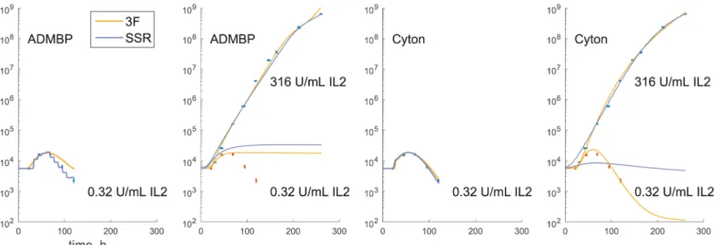
variables changed, e.g., T cells proliferate in the presence of different concentrations of interleu-kin 2 (IL2). A response model can be then fit simultaneously to the data for all concentrations, where certain proliferation parameters (e.g., starting cell number) are constrained to remain the same across concentrations. In addition, in a multiconcentration experiment, it is common to observe large differences in cell numbers, where weak stimulation results in rapid population extinction, whereas string stimulation leads to a considerable growth. The use of SSR for such data may result in the low concentration data being essentially ignored (Fig 6).
So far, we have considered ADMBP and Cyton response models. Note that for a given data-set, an ideal response model would be the one that predicts measurement means. We therefore,
also implemented such a hypothetical model, and assumed that it haskrespparameters, where
krespwas set to 1%, 5% or 10% from the number of data points. We then embedded this model
within 3F, SSR, or LVS, and computed AICc for each dataset. We find that overall 3F offers the best explanation for the data (S2 Table).
Finally, note that embedding a response model within a measurement model may increase the total number of parameters. Additional parameters introduced by the 3F model are
dis-cussed inS2 Text. All of them, except one (denotedε) are estimated from the data. In our
eval-uation, we use the default valueε= 50. Further, inS2 Textwe discuss situations when fitting
is not expected to be sensitive to the choice ofε. Indeed, when we repeated fitting several times,
each time starting from the same initial parameter guess, but varyingεfrom 0.25εto 4ε, we
obtained similar results (S5 Fig). Overall, we conclude that the 3F measurement model offers a reliable probabilistic way of fitting response models to lymphocyte data. This measurement model tends to explain the data better than previous models, and does not suffer certain unde-sirable effects, such as data capping or imbalanced fitting between data for different stimuli concentrations.
Discussion
Flow cytometry is a popular tool for quantifying lymphocyte responses—and fitting
research groups have adopted different sets of assumptions for fitting to the same type of data. A further inconsistency with these methods is that fitting is sometimes performed using a heu-ristic objective function, while the resulting fits are compared using a probabilistic criterion.
Here we addressed this problem by assessing commonly used assumptions on measure-ments. We collected data representative of a wide range of experimental conditions and found
an empirical power law relationυ=αμβ, whereμis the sample mean andυis the sample
vari-ance for measured replicates from each group (e.g., a sample of repeated measurements for
cells in generation 2 at 24 hours). From our data, we estimatedβto fall between 1.3 and 1.8 (it
varies for different datasets) which violates common assumptions of the variance being con-stant (SSR) or scaling linearly with the mean (LVS), as well as the assumption of log-normal measurements (LogNrm).
Mathematically, the observed mean-variance relation is equivalent to the well-known
empirical Taylor’s law that has been found to apply in various biological domains [31–33].
Taylor described this law in an ecological context, counting the number of species per unit area, and related the power exponent to the degree of aggregation of the organisms. The emergence of a power law in the context of lymphocyte experiments is presumably due to completely different reasons that are yet to be established. It is also likely that these reasons pri-marily reflect idiosyncrasies of flow cytometry/gating workflow rather than biology, in which case, the main interest in the power-law relation is for model fitting. Indeed, in our
measure-ment model we estimateαandβfrom data which enables us to achieve more reliable model
fit-ting compared to methods whereαandβare fixed.
Multiconcentration fitting is an emerging task where a range of conditions, such as titration of a cytokine, is tested within a single experiment. A fit is then performed simultaneously to the results of all conditions, with some parameters (e.g., death rate) constrained to remain constant across conditions. Since cell counts are likely to differ by several orders of magnitude for differ-ent concdiffer-entrations it is important to balance the contribution of each data point. Allowing power law scaling helps to achieve this balance in our measurement model.
In our measurement model, the power law exponent is estimated independently for each dataset, but is fixed for a dataset. Furthermore, we assume a single-component MVN distribution
Fig 6. SSR is not suitable for multiconcentration fitting.ADMBP and Cyton models are fitted to a low and high stimulation condition selected fromt–il2
dataset. When a low concentration data is fitted independently, SSR can be used to fit models. However, when both concentrations are fitted simultaneously, SSR tends to ignore low concentration data because the range of these data is comparable to measurement noise for the high concentration measurements. At the same time, 3F tends to produce more balanced fits, because it scales measurement variance in accordance to the mean.
for all measurements. This decision was made in view that most of lymphocyte response models assume a homogeneous population of cells with a fixed parameter vector describing the
popula-tion [4,7,11]. Our evaluation suggests that even this simple setup can lead to improvements
compared to the state-of-the-art. At the same time, future and more advanced measurement models can consider, for example, specifying a distribution over the power law exponent, or a mixture model for measurements as a consequence of presence of different cell types within a population. Another possibility to explore is letting the power exponent to vary over time (S6 Fig). Our current work contributes an evaluation framework, and a new baseline facilitating progress in the field.
In addition to the applications detailed above, we have addressed the theoretical foundation of our method. We justify the choice of the measurement distribution using the maximum entropy principle. This is a well-known principle in the field of signal processing, and here we introduce this idea in the context of quantifying lymphocyte responses. Further, the theoretical development of our model is not specific to lymphocytes and potentially can be applied to flow cytometry experiments involving other cell types. In regards to lymphocyte responses, our work lays a foundation for a consistent handling of flow cytometry data to support ongoing and future model development in the field.
Materials and Methods
Mice, culture preparation, flow cytometry
Our dataset collection comprises 6 datasets from previous studies, and 4 datasets performed for this study, and outlined below. All experiments were performed under the approval of the Walter and Eliza Hall Institute (WEHI) Animal Ethics Committee. All mice used were main-tained in specific pathogen-free conditions at WEHI animal facilities (Kew, Bundoora, and Parkville, Victoria, Australia) in accordance with WEHI animal ethics committee regulations. All transgenic mouse strains used were on a C57BL/6 background.
b–bimko. Small resting B cells, isolated from spleens from one B6/del339-/- (C57BL/6, deficient for Bim) and one B6/del339+/- (heterozygous for Bim deficiency) were labelled with
5μM CTV and stimulated with 3μM CpG 1668 at 10,000 cells per well. Cell isolation procedure
and culture conditions were as described previously [21]. Measurements were performed in 9 replicates.
b–gfpandb–tot. Small, resting naÃve B cells were isolated from the spleens of
Blimp-1GFP/+reporter mice at 10
–12 weeks of age using a percoll gradient (65/80% interface) and
magnetic-activated cell sorting B cell isolation kit (Miltenyi). Cells were stained with 7.5μM
CTV and placed into culture with 10μg/mLanti-CD40 antibody (1C10) and 1000 U/mL IL-4.
Cells were bulk cultured at 100,000 cells/mL for 3 days (under 37°C, 5%CO2, and humidity
control) before being harvested and plated at 20,000 cells per 200μLin triplicate wells, in the presence of stimuli as before, as well as cell-cycle inhibiting drugs at various concentrations (b–gfp: etoposide, purvalanol A and vincristine;b–tot: etoposide, purvalanol A and
aphidico-lin). Further, 6,000 fluorescent beads were added to each well in 10μLjust prior to analysis at day 4 (b–gfp) or day 7 (b–tot) on the BD Canto flow cytometer, along with 0.5μMof
propi-dium iodide.
t–n4. Naive CD8 T cells were isolated from the lymph nodes of approximately 12 weeks
old OT-1 mice using a MACS CD8 II isolation kit. Anti-CD44-biotin antibody was added to biotinylated purification cocktail to remove memory T cells. Purified naive CD8 T cells were
labelled with 5μM CTV and cultured at 10,000 cells /well in the presence of 1ng/mL IL-7 and
0.2% propidium iodide were added to each well immediately prior to analysis on a BD Canto flowcytometer. Calculation of total cell numbers and cell numbers per division are described in [4].
Datasetsb–cd40,b–cpg, andb–lpswere obtained from the authors of [24]. These data are
shown, respectively, in Supplementary Figures S4, S2 and S3 in reference [24]. Datasetst–il2,
t–vv–qsc, andt–vv–totwere obtained from the authors of [4]. These data are shown,
respec-tively, in Figures 2C, 1D and 4D in reference [4].
Statistical analysis of the datasets
For the statistics presented inS1 Table, Pearson correlation p-values were computed using a
Student’s t distribution for a transformation of the correlation. Power law parameters were
esti-mated using linear regression with two parameters (slope and intercept) on the log-log scale. This estimation was performed separately for each dataset. Confidence intervals for linear regression were estimated asbi±t(1−α/2,n−c)SE(bi), whereSE(bi) is the standard error of the esti-mate,t(1−α/2,n−c)is the 100 × (1−α/2) percentile oftdistribution withn−cdegrees of freedom,
nis the number of observations, andcis the number of regression coefficients.
Parameter estimation
Parameter estimation (model fitting) was performed as an optimization that maximizes the
likelihood (for SSR, LogNrm, and LVS models) or maximuma posterioriprobability (for 3F) as
a function ofθ. The optimization was implemented and tested in a MATLAB 2014b
environ-ment using the impleenviron-mentation of the interior point algorithm provided by the environenviron-ment
(via standardfminconfunction). The optimization result depends on the starting pointθ02Θ
[28], and we repeated optimization independently 10 times with randomly generated starting vectors. Random starting vectors have each of their components sampled independently from other components uniformly from the range of valid parameter values provided by the user.
For multiconcentration fitting, some parameters can befixed, i.e., constrained to remain equal
across concentrations. These user-defined parameter ranges, as well as lists of fixed parameters
can be found inS1 Dataset. Each of the runs returned an estimate for the optimal parameter
vector, and the final result was the best vector across all runs. Source code for the fitting process
can be found inS1 File. Note that LVS and LogNrm involve additional parameters, and we
usedε= 50 for LVS, andc¼ ffiffiffiffiffi
50
p
for LogNrm.
Supporting Information
S1 Dataset. Experimental data used in this work.Detail of data format can be found within the archive.
(ZIP)
S1 Fig. Variance of log-transformed data is not constant.Plots show means and variances of log-transformed data for each of the datasets. Variance can span several orders of magnitude and it depends on the mean. This violates assumptions of LogNrm approach.
(PDF)
S2 Fig. Model fits obtained using different measurement models.ADMBP model was fitted
tot–n4data using different measurement models. Resulting AICc scores are 2320.7 (3F),
4046.2 (SSR), 4166.8 (LogNrm), and 311694.4 (LVS). For the fit obtained using LogNrm model, AICc was computed using SSR model.
S3 Fig. Model fits obtained using different measurement models.Cyton model was fitted to
b–bimkodata using different measurement models. Resulting AICc scores are 8238.4 (3F),
10326.0 (SSR), 11602.7 (LogNrm), and 436803.5 (LVS). For the fit obtained using LogNrm model, AICc was computed using SSR model.
(PDF)
S4 Fig. Model fits obtained using different measurement models.ADMBP model was fitted
tob–bimkodata using different measurement models. Resulting AICc scores are 9085.5 (3F),
12024.4 (SSR), 13125.6 (LogNrm), and 2674181.0 (LVS). For the fit obtained using LogNrm model, AICc was computed using SSR model.
(PDF)
S5 Fig. Fitting is not sensitive to the choice of parameterε.Cyton model was fitted to a rep-resentative dataset (in this case,b–lps), and the fitting was repeated several times using different εranging from 0.25εto 4ε, whereε= 50. The choice ofεmade little difference to results. Note that this is a multiconcentration dataset, and the fit was performed to all concentrations simultaneously. Further, each time point contains breakdown of the number of cells per gener-ation, but in the figure, only the total number are shown.
(PDF)
S6 Fig. Analysis of the power law exponent over time.Each point shows the power law expo-nent estimated from samples from a particular time point. Any given time point comprises sev-eral measurement samples (e.g., number of cells in division 1 measured 3 times is one sample; number of cells in division 2 measured 3 times is another sample, etc.). Each sample is then summarized by sample mean and sample variance, a power law relation between mean and variance is fit to data from a single time point, and the exponent is plotted against time. We
used only time points with more than 3 samples. Datasetsb-gfpandb-totdid not have time
points that satisfy this criterion. Overall, there appears to be a slight increasing trend for each dataset, and this observation can be exploited in future measurement models.
(PDF)
S1 File. Source code for parameter estimation.MATLAB implementation of 3F measure-ment model, Cyton response model, as well as fitting and data analysis routines.
(ZIP)
S2 File. Compiled executables.These files can be used to reproduce figures and tables from this paper, as well as for fitting to new data. Please refer toreadme.txtfor details.
(ZIP)
S1 Table. Statistics computed for experimental data.For each dataset, power law was fitted as a linear regression on the log-log scale, and table shows the parameters of the regression. In the fitted line, slope corresponds to the power exponent and intercept corresponds to the loga-rithm of the scaling coefficient. Next, table shows p-values for the sign test for residuals of the linear regression, and p-values of Pearson correlation between sample means and variances. The final column shows p-values for Pearson correlation between sample means and variances for log-transformed data. The last row shows statistics for the combined dataset, and it contains p-value for Kruskal-Wallis test.
(XLSX)
S2 Table. Comparing performance of measurement models.For each dataset, we consider the fit matching all measurement means, produced by a hypothetical response model with
number of data points. Measurement model performance was assessed using AICc. Overall, 3F outperforms other models.
(XLSX)
S1 Text. Previous measurement models.Formal description of some previously proposed measurement models.
(PDF)
S2 Text. Description of our measurement model.Complete formal description of the pro-posed measurement model and parameter estimation methods.
(PDF)
S3 Text. Testing normality of the data.Normality tests suggest that a MVN distribution is a reasonable approximation for the distribution of measurements. Unless otherwise stated, p-values are given for Lilliefors test.
(PDF)
Acknowledgments
We would like to acknowledge Cameron Wellard, Ken Duffy and Vijay Subramanian for inspiring discussions on the mystery of parameter estimation and differential entropy. We
would also like to thank an anonymous reviewer for suggesting the analysis presented inS6
Fig. This work was made possible through Victorian State Government Operational Infrastruc-ture Support and Australian Government National Health and Medical Research Council Independent Research Institutes Infrastructure Support Scheme.
Author Contributions
Conceived and designed the experiments: AK DP JFM MRD SH JHSZ. Performed the experi-ments: SH JHSZ. Analyzed the data: AK JMM PDH. Wrote the paper: AK DP JFM MRD SH JHSZ JMM PDH.
References
1. Duffy K, Wellard C, Markham J. Activation-induced B cell fates are selected by intracellular stochastic competition. Science. 2012; 335(6066):338–341. PMID:22223740
2. Inokuma MS, Maino VC, Bagwell CB. Probability state modeling of memory CD8(+) T-cell differentia-tion. Journal of immunological methods. 2013 Nov; 397(1–2):8–17. doi:10.1016/j.jim.2013.08.003 PMID:23954473
3. Sciammas R, Li Y, Warmflash A, Song Y, Dinner AR, Singh H. An incoherent regulatory network archi-tecture that orchestrates B cell diversification in response to antigen signaling. Molecular systems biol-ogy. 2011 May; 7(495):495. Available from:http://www.pubmedcentral.nih.gov/articlerender.fcgi?artid = 3130558&tool = pmcentrez&rendertype = abstract. doi:10.1038/msb.2011.25PMID:21613984 4. Marchingo JM, Kan A, Sutherland RM, Duffy KR, Wellard CJ, Belz GT, et al. Antigen affinity,
costimula-tion, and cytokine inputs sum linearly to amplify T cell expansion. Science. 2014 Nov; 346(6213):1123– 1127. doi:10.1126/science.1260044PMID:25430770
5. Couzin-Frankel J. Cancer Immunotherapy. Science. 2013; 342(6165):1432–1433. doi:10.1126/ science.342.6165.1432PMID:24357284
6. Perfetto SP, Chattopadhyay PK, Roederer M. Seventeen-colour flow cytometry: unravelling the immune system. Nature reviews Immunology. 2004; 4(8):648–655. doi:10.1038/nri1416PMID: 15286731
7. De Boer RJ, Perelson AS. Quantifying T lymphocyte turnover. Journal of theoretical biology. 2013 Jan;. doi:10.1016/j.jtbi.2012.12.025PMID:23313150
9. León K, Faro J, Carneiro J. A general mathematical framework to model generation structure in a popu-lation of asynchronously dividing cells. Journal of theoretical biology. 2004 Aug; 229(4):455–76. doi: 10.1016/j.jtbi.2004.04.011PMID:15246784
10. Luzyanina T, Cupovic J, Ludewig B, Bocharov G. Mathematical models for CFSE labelled lymphocyte dynamics: asymmetry and time-lag in division. Journal of mathematical biology. 2013 Dec; PMID: 24337680
11. Miao H, Jin X, Perelson AS, Wu H. Evaluation of multitype mathematical models for CFSE-labeling experiment data. Bulletin of Mathematical Biology. 2012 Feb; 74(2):300–326. Available from:http:// www.pubmedcentral.nih.gov/articlerender.fcgi?artid = 3196768&tool = pmcentrez&rendertype = abstract. doi:10.1007/s11538-011-9668-yPMID:21681605
12. Shokhirev MN, Hoffmann A. FlowMax: A Computational Tool for Maximum Likelihood Deconvolution of CFSE Time Courses. PloS one. 2013 Jan; 8(6):e67620. Available from:http://www.pubmedcentral.nih. gov/articlerender.fcgi?artid = 3694893&tool = pmcentrez&rendertype = abstract. doi:10.1371/journal. pone.0067620PMID:23826329
13. Yates A, Chan C, Strid J, Moon S, Callard R, George AJT, et al. Reconstruction of cell population dynamics using CFSE. BMC bioinformatics. 2007; 8:196. doi:10.1186/1471-2105-8-196PMID: 17565685
14. Lyons aB, Parish CR. Determination of lymphocyte division by flow cytometry. Journal of immunological methods. 1994; 171(94):131–137. doi:10.1016/0022-1759(94)90236-4PMID:8176234
15. Quah BJC, Parish CR. New and improved methods for measuring lymphocyte proliferation in vitro and in vivo using CFSE-like fluorescent dyes. Journal of Immunological Methods. 2012; 379(1–2):1–14. doi:10.1016/j.jim.2012.02.012PMID:22370428
16. Revy P, Sospedra M, Barbour B, Trautmann a. Functional antigen-independent synapses formed between T cells and dendritic cells. Nature immunology. 2001; 2(10):925–931. doi:10.1038/ni713 PMID:11561183
17. Hyrien O, Mayer-Pröschel M, Noble M, Yakovlev A. A stochastic model to analyze clonal data on multi-type cell populations. Biometrics. 2005; 61(1):199–207. doi:10.1111/j.0006-341X.2005.031210.x PMID:15737094
18. Hawkins ED, Turner ML, Dowling MR, van Gend C, Hodgkin PD. A model of immune regulation as a consequence of randomized lymphocyte division and death times. Proceedings of the National Acad-emy of Sciences of the United States of America. 2007 Mar; 104(12):5032–7. Available from:http:// www.pubmedcentral.nih.gov/articlerender.fcgi?artid = 1821128&tool = pmcentrez&rendertype = abstract. doi:10.1073/pnas.0700026104PMID:17360353
19. Kallies A, Hasbold J, Tarlinton DM, Dietrich W, Corcoran LM, Hodgkin PD, et al. Plasma cell ontogeny defined by quantitative changes in blimp-1 expression. The Journal of experimental medicine. 2004 Oct; 200(8):967–77. Available from:http://www.pubmedcentral.nih.gov/articlerender.fcgi?artid = 2211847&tool = pmcentrez&rendertype = abstract. doi:10.1084/jem.20040973PMID:15492122 20. Sakaue-Sawano A, Kurokawa H, Morimura T, Hanyu A, Hama H, Osawa H, et al. Visualizing
spatio-temporal dynamics of multicellular cell-cycle progression. Cell. 2008; 132(3):487–498. doi:10.1016/j. cell.2007.12.033PMID:18267078
21. Hawkins ED, Markham JF, McGuinness LP, Hodgkin PD. A single-cell pedigree analysis of alternative stochastic lymphocyte fates. Proceedings of the National Academy of Sciences of the United States of America. 2009; 106(32):13457–13462. doi:10.1073/pnas.0905629106PMID:19633185
22. Subramanian VG, Duffy KR, Turner ML, Hodgkin PD. Determining the expected variability of immune responses using the cyton model. Journal of Mathematical Biology. 2008 Jun; 56(6):861–892. Avail-able from:http://www.ncbi.nlm.nih.gov/pubmed/17982747http://www.springerlink.com/index/ 419W462T31U11661.pdf. doi:10.1007/s00285-007-0142-2PMID:17982747
23. Hasbold J, Gett aV, Rush JS, Deenick E, Avery D, Jun J, et al. Quantitative analysis of lymphocyte dif-ferentiation and proliferation in vitro using carboxyfluorescein diacetate succinimidyl ester. Immunology and Cell Biology. 1999; 77(6):516–522. doi:10.1046/j.1440-1711.1999.00874.xPMID:10571672 24. Hawkins ED, Turner ML, Wellard CJ, Zhou JHS, Dowling MR, Hodgkin PD. Quantal and graded
stimu-lation of B lymphocytes as alternative strategies for regulating adaptive immune responses. Nature communications. 2013 Sep; 4:2406. doi:10.1038/ncomms3406PMID:24009041
25. Banks HT, Kapraun DF, Thompson WC, Peligero C, Argilaguet J, Meyerhans A. A novel statistical anal-ysis and interpretation of flow cytometry data. Journal of biological dynamics. 2013 Jan; 7(1):96–132. Available from:http://www.pubmedcentral.nih.gov/articlerender.fcgi?artid = 3753657&tool = pmcentrez&rendertype = abstract. doi:10.1080/17513758.2013.812753PMID:23826744
27. Hawkins ED, Hommel M, Turner ML, Battye FL, Markham JF, Hodgkin PD. Measuring lymphocyte pro-liferation, survival and differentiation using CFSE time-series data. Nature protocols. 2007 Jan; 2 (9):2057–67. doi:10.1038/nprot.2007.297PMID:17853861
28. Baker C, Bocharov G. Computational modelling with functional differential equations: Identification, selection, and sensitivity. Applied Numerical.. . .2005;Available from:http://www.sciencedirect.com/
science/article/pii/S0168927404001308.
29. Jaynes ET. Information Theroy and Statistical Mechanics. The Physical Review. 1957; 106(4):620– 630. doi:10.1103/PhysRev.106.620
30. Dempster A. Covariance selection. Biometrics. 1972;Available from:http://www.jstor.org/stable/ 2528966.
31. Taylor LR. Aggregation, Variance and the Mean. Nature. 1961; 189(4766):732–735. doi:10.1038/ 189732a0
32. Kendal WS. A stochastic model for the self-similar heterogeneity of regional organ blood flow. Proceed-ings of the National Academy of Sciences of the United States of America. 2001; 98(3):837–841. doi: 10.1073/pnas.98.3.837PMID:11158557