www.hydrol-earth-syst-sci.net/15/1835/2011/ doi:10.5194/hess-15-1835-2011
© Author(s) 2011. CC Attribution 3.0 License.
Earth System
Sciences
River flow time series using least squares support vector machines
R. Samsudin1, P. Saad1, and A. Shabri2
1Faculty of Computer Science and Information System, Universiti Teknologi Malaysia, 81310, Skudai, Johor, Malaysia 2Faculty of Science, Universiti Teknologi Malaysia, 81310, Skudai, Johor, Malaysia
Received: 27 April 2010 – Published in Hydrol. Earth Syst. Sci. Discuss.: 23 June 2010 Revised: 25 May 2011 – Accepted: 29 May 2011 – Published: 17 June 2011
Abstract. This paper proposes a novel hybrid forecast-ing model known as GLSSVM, which combines the group method of data handling (GMDH) and the least squares sup-port vector machine (LSSVM). The GMDH is used to de-termine the useful input variables which work as the time series forecasting for the LSSVM model. Monthly river flow data from two stations, the Selangor and Bernam rivers in Selangor state of Peninsular Malaysia were taken into con-sideration in the development of this hybrid model. The per-formance of this model was compared with the conventional artificial neural network (ANN) models, Autoregressive In-tegrated Moving Average (ARIMA), GMDH and LSSVM models using the long term observations of monthly river flow discharge. The root mean square error (RMSE) and co-efficient of correlation (R) are used to evaluate the models’ performances. In both cases, the new hybrid model has been found to provide more accurate flow forecasts compared to the other models. The results of the comparison indicate that the new hybrid model is a useful tool and a promising new method for river flow forecasting.
1 Introduction
River flow forecasting is one of the most important compo-nents of hydrological processes in water resource manage-ment. Accurate estimations for both short and long term forecasts of river flow can be used in several water engi-neering problems such as designing flood protection works for urban areas and agricultural land and optimizing the al-location of water for different sectors such as agriculture, municipalities, hydropower generation, while ensuring that
Correspondence to:R. Samsudin ([email protected])
environmental flows are maintained. The identification of highly accurate and reliable river flow models for future river flow is an important precondition for successful planning and management of water resources.
The second approach which is the data-driven modelling is based on extracting and re-using information that is implic-itly contained in the hydrological data without directly tak-ing into account the physical laws that underlie the rainfall-runoff processes. In river flow forecasting applications, data-driven modelling using historical river flow time series data is becoming increasingly popular due to its rapid development times and minimum information requirements (Adamowski and Sun, 2010; Atiya et al., 1999; Lin et al., 2006; Wang et al., 2006, 2009; Wu et al., 2009; Firat and Gungor, 2007; Fi-rat, 2008; Kisi, 2008, 2009). Although the data-driven mod-elling may lack the ability to provide physical interpretation and insight of the catchment processes but it is able to pro-vide relatively accurate flow forecasts.
Computer science and statistics have improved the data-driven modelling approaches for discovering patterns found in water resources time series data. Much effort has been de-voted over the past several decades to the development and improvement of time series prediction models. One of the most important and widely used time series models is the autoregressive integrated moving average (ARIMA) model. The popularity of the ARIMA model is due to its statistical properties as well as the well known Box-Jenkins method-ology. Literature on the extensive applications and reviews of ARIMA model proposed for modeling of water resources time series are indicative of researchers’ preference (Yurekli et al., 2004; Muhamad and Hassan, 2005; Huang et al., 2004; Modarres, 2007; Fernandez and Vega, 2009; Wang et al., 2009). However, the ARIMA model provides only a rea-sonable level of accuracy and suffer from the assumptions of stationary and linearity.
The data-driven models such as artificial neural networks (ANN) have recently been accepted as an efficient alternative tool for modelling a complex hydrologic system compared with the conventional methods and is widely used for predic-tion (Karunasinghe and Liong, 2006; Rojas et al., 2008; Ca-mastra and Colla, 1999; Han and Wang, 2009; Abraham and Nath, 2001). ANN has emerged as one of the most success-ful approaches in the various areas of water-related research, particular in hydrology. A comprehensive review of the ap-plication of ANN in hydrology was presented by the ASCE Task Committee report (2000). Some specific applications of ANN to hydrology include modelling river flow forecast-ing (Dollforecast-ing and Varas, 2003; Muhamad and Hassan, 2005; Kisi, 2008; Wang et al., 2009; Keskin and Taylan, 2009), rainfall-runoff modeling (De Vos and Rientjes, 2005; Hsu et al., 1995; Shamseldin, 1997; Hung et al., 2009), ground wa-ter management (Affandi and Watanabe, 2007; Birkinshaw et al., 2008) and water quality management (Maier and Dandy, 2000). However, there are some disadvantages of the ANN. Its network structure is hard to determine and this is usually determined by using a trial-and-error approach (Kisi, 2004). More advanced artificial intelligent (AI) is the support vec-tor machine (SVM) proposed by Vapnik (1995) and his co-workers in 1995 based on the statistical learning theory, has
gained the attention of many researchers. SVM has been applied to time series prediction with promising results as seen in the works of Tay and Cao (2001), Thiessen and Van Brakel (2003) and Misra et al. (2009). Several studies have also been carried out using SVM in hydrological and water resources planning (Wang et al., 2009; Asefa et al., 2006; Lin et al., 2006; Dibike et al., 2001; Liong and Sivapragasam, 2002; Yu et al., 2006). The standard SVM is solved using quadratic programming methods. However, this method is often time consuming and has a high computational burden because of the required constrained optimization program-ming.
Least squares support vector machines (LSSVM), as a modification of SVM was introduced by Suykens and Van-dewalle (1999). LSSVM is a simplified form of SVM that uses equality constraints instead of inequality constraints and adopts the least squares linear system as its loss function, which is computationally attractive. Besides that, it also has good convergence and high precision. Hence, this method is easier to use than quadratic programming solvers in SVM method. Extensive empirical studies (Wang and Hu, 2005) have shown that LSSVM is comparable to SVM in terms of generalization performance. The major advantage of LS-SVM is that it is computationally very cheap besides having the important properties of the SVM. LSSVM has been suc-cessfully applied in diverse fields (Afshin et al., 2007; Lin et al., 2005; Sun and Guo, 2005; Gestel et al., 2001). How-ever, in the water resource filed, this LSSVM method has received very little attention and there are only a few applica-tions of LSSVM to modeling of environmental and ecolog-ical systems such as water quality prediction (Yunrong and Liangzhong, 2009).
One sub-model of ANN is a group method data han-dling (GMDH) algorithm which was first developed by Ivakhnenko (1971). This is a multivariate analysis method for modeling and identification of complex systems. The main idea of GMDH is to build an analytical function in a feed-forward network based on a quadratic node transfer function whose coefficients are obtained by using the re-gression technique. This model has been successfully used to deal with uncertainty and linear or nonlinearity systems in a wide range of disciplines such as engineering, science, economy, medical diagnostics, signal processing and con-trol systems (Tamura and Kondo, 1980; Ivakhnenko and Ivakhnenko, 1995; Voss and Feng, 2002). In water resource, the GMDH method has received very attention and only a few applications to modeling of environmental and ecolog-ical systems (Chang and Hwang, 1999; Onwubolu et al., 2007; Wang et al., 2005) have been carried out.
are extremely complex to be modeled using these simple ap-proaches especially when a high level of accuracy is required. Different data-driven models can achieve success which is different from each other as each would capture various pat-terns of data sets, and numerous authors have demostrated that a hybrid based on the predictions of several models fre-quently results in higher prediction accuracy than the pre-diction of an individual model. The hybrid model is widely used in diverse fields, such economics, business, statistics and metorology (Zhang, 2003; Jain and Kumar, 2006; Su et al., 1997; Wang et al., 2005; Chen and Wang, 2007; On-wubolu, 2008; Yang et al., 2006). Many studies have also developed a number of hybrid forecasting models in hydro-logical processes in order to improve prediction accuracy as reported in the literature. See and Openshaw (2009) pro-posed a hybrid model that combines fuzzy logic, neural net-works and statistical-based modeling to form an integrated river level forecasting methodology. Another study by Wang et al. (2005) presented a hybrid methodology to exploit the unique strength of GMDH and ANN models for river flow forecasting. Besides that Jain and Kumar (2006) proposed a hybrid approach for time series forecasting using monthly stream flow data at Colorado river. Their study indicated that the approach of combining the strengths of the conventional and ANN techniques provided a robust modeling framework capable of capturing the nonlinear nature of the complex time series, thus producing more accurate forecasts.
In this paper, a novel hybrid approach combining GMDH model and LSSVM model is developed to forecast river flow time series data. The hybrid model combines GMDH and LSSVM into a methodology known as GLSSVM. In the first phase, GMDH is used to determine the useful input variables from the under study time series. Then, in the second phase, the LSSVM is used to model the generated data by GMDH model to forecast the future value of the time series. To ver-ify the application of this approach, the hybrid model was compared with ARIMA, ANN, GMDH and LSSVM mod-els using two river flow data sets: the Selangor and Bernam rivers located in Selangor, Malaysia.
2 Individual forecasting models
This section presents the ARIMA, ANN, GMDH and LSSVM models used for modeling time series. The reason for choosing these models in this study were because these methods have been widely and successfully used in forecast-ing time series.
2.1 The Autoregressive Integrated Moving Average (ARIMA) models
The ARIMA models introduced by Box and Jenkins (1970), has been one of the most popular approaches in the analysis of time series and prediction. The general ARIMA models
are compound of a seasonal and non-seasonal part are repre-sented as:
φp(B) 8P Bs(1−B)d 1−BsD xt = θq(B) 2Q Bsat(1)
whereφ (B)andθ (B)are polynomials of orderpandq, re-spectively; 8(Bs)and2(Bs)are polynomials inBs of de-greesP andQ, respectively;pis the order of non-seasonal auto regression;dis the number of regular differencing;qis the order of the non-seasonal moving average;P is the order of seasonal auto regression;Dis the number of seasonal dif-ferencing;Qis the order of seasonal moving average; and s length of season. Random errors,at are assumed to be
inde-pendently and identically distributed with a mean of zero and a constant variance ofσ2. The order of an ARIMA model is represented by ARIMA (p,d,q) and the order of an seasonal ARIMA model is represented by ARIMA(p,d,q)×(P,D,
Q)s. The term (p,d,q) is the order of the non-seasonal part and (P,D,Q)sis the order of the seasonal part.
The Box-Jenkins methodology is basically divided into four steps: identification, estimation, diagnostic checking and forecasting. In the identification step, transformation is often needed to make time series stationary. The behavior of the autocorrelation (ACF) and partial autocorrelation func-tion (PACF) is used to see whether the series is stafunc-tionary or not, seasonal or non-seasonal. The next step is choos-ing a tentative model by matchchoos-ing both ACF and PACF of the stationary series. Once a tentative model is identified, the parameters of the model are estimated. Then, the last step of model building is the diagnostic checking of model adequacy. Basically this is done to check if the model as-sumptions about the error, at are satisfied. If the model is
not adequate, a new tentative model should be identified fol-lowed by the steps of parameter estimation and model verifi-cation. This process is repeated several times until a satisfac-tory model is finally selected. The forecasting model would then be used to compute the fitted values and forecasts val-ues.
To be a reliable forecasting model, the residuals must sat-isfy the requirements of a white noise process i.e. indepen-dent and normally distributed around a zero mean. In order to determine whether the river flow time series are independent, two diagnostic checking statistics using the ACF of residuals of the series were carried out (Brockwell and Davis, 2002). The first one is the correlograms drawn by plotting the ACF of residual against a lag number. If the model is adequate, the estimated ACF of the residual is independent and distributed approximately normally about zero. The second one is the Ljung-Box-Pierce statistics which are calculated for the dif-ferent total numbers of successive lagged ACF of residual in order to test the adequacy of the model.
values (Akaike, 1974). Mathematical formulation of AIC is defined as:
AIC = ln Pn
t=1e2t n
!
+ 2p
n (2)
wherepis the number of parameters andnis the periods of data.
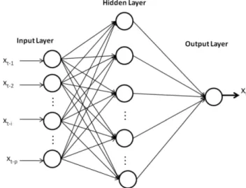
2.2 The Artificial Neural Network (ANN) model The ANN models based on flexible computing have been extensively studied and used for time series forecasting in many areas of science and engineering since early 1990s. The ANN is a mathematical model which has a highly con-nected structure similar to brain cells. This model has the ca-pability to execute complex mapping between input and out-put and could form a network that approximates non-linear functions. A single hidden layer feed forward network is the most widely used model form for time series modeling and forecasting (Zhang et al., 1998). This model usually consists of three layers: the first layer is the input layer where the data are introduced to the network followed by the hidden layer where data are processed and the final or output layer is where the results of the given input are produced. The structure of a feed-forward ANN is shown in Fig. 1.
The output of the ANN assuming a linear output neuron
j, a single hidden layer withhsigmoid hidden nodes and the output variable (xt) is given by:
xt = g
Xh
j=1wj f sj
+bk
(3) whereg(.)is the linear transfer function of the output neuron
k andbk is its bias, wj is the connection weights between
hidden layers and output units,f (.)is the transfer function of the hidden layer (Coulibaly and Evora, 2007). The transfer functions can take several forms and the most widely used transfer functions are:
Log−sigmoid:f (si) =logsig(si) =
1 1 + exp(−si)
(4) Linear:f (si) = purelin(si) = si
Hyperbolic tangent sigmoid:f (si) = tansig(si)
= 2
1 + exp(−2si)
−1
wheresi=Pni=1 wi xi is the input signal referred to as the
weighted sum of incoming information.
In a univariate time series forecasting problem, the inputs of the network are the past lagged observations (xt−1, xt−2, ..., xt−p) and the output is the predicted value
(xt) (Zhang et al., 2001). Hence the ANN of Eq. (3) can be
written as:
xt = g xt−1, xt−2, ..., xt−p,w
+εt (5)
Fig. 1.Architecture of three layers feed-forward back-propagation ANN.
wherewis a vector of all parameters andg(.)is a function determined by the network structure and connection weights. Thus, in some senses, the ANN model is equivalent to a non-linear autoregressive (NAR) model.
Several optimization algorithms can be used to train the ANN. Among the training algorithms available, the back-propagation has been the most popular and widely used al-gorithm (Zou et al., 2007). In a back-propagation network, the weighted connections only feed activations in the for-ward direction from an input layer to the output layer. The-ses interconnections are adjusted using an error convergence technique so that response of the network would be the best matches as well as the desired responses.
2.3 The Least Square Support Vector Machines (LSSVM) model
The LSSVM is a new technique for regression. In this tech-nique, the predictor is trained by using a set of time series historic values as inputs and a single output as the target value. In the following sections, discussions on how LSSVM is used for time series forecasting is presented.
The first step would be to consider a given training set of
ndata points{xi, yi}ni=1with input dataxi∈Rn,pis the total
number of data patterns and output yi∈R. SVM
approxi-mates the function in the following form:
y(x) = wT φ (x) +b (6)
whereφ (x)represents the high dimensional feature spaces which is mapped in a non-linear manner from the input space
x. In the LSSVM for function estimation, the optimization problem is formulated (Suykens et al., 2002) as:
minJ (w, e) = 1 2
wT w+ γ 2
n X
i=1
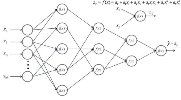
Fig. 2.Architecture of GMDH.
Subject to the equality constraints:
y(x) = wT φ (xi) +b +ei i = 1,2, ..., n (8)
The solution is obtained after constructing the Lagrange: L(w, b, e, α)= J (w, e)−
n
X
i=1
αi{wTφ (xi)+b+ei −yi} (9) With Lagrange multipliersαi. The conditions for optimality
are:
∂L
∂w = 0 →
w =
N X
i=1
αiφ (xi),
∂L
∂b = 0 →
N X
i=1
αi = 0,
∂L ∂ei
= 0 → αi = γ ei, ∂L
∂αi
= 0 → wT φ (xi)+b +ei −yi = 0, (10) fori= 1, 2, ..., n. After elimination ofei andw, the solution
is given by the following set of linear equations:
0 1T
1φ (xi)T φ (xi) +γ−1I b α
=
0
y
(11) wherey=[y1, ..., yn],1=[1, ..., 1],α=[α1, ..., αn].
Ac-cording to Mercer’s condition, the kernel function can be de-fined as:
K xi, xj
= φ (xi)T φ xj
, i, j = 1,2, ..., n (12)
This finally leads to the following LSSVM model for func-tion estimafunc-tion:
y(x) =
n X
i=1
αi K xi, xj +b (13)
whereαi,bare the solution to the linear system. Any
func-tion that satisfies Mercer’s condifunc-tion can be used as the kernel function. The choice of the kernel functionK(.,.)has sev-eral possibilities.K(xi, xj)is defined as the kernel function.
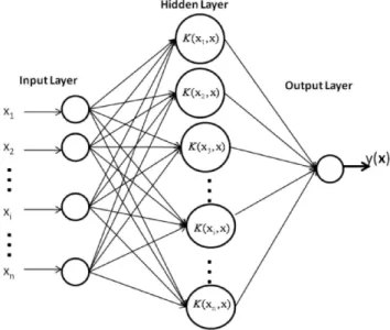
The value of the kernel is equal to the inner product of two vectorsXi andXj in the feature spaceφ (xi)andφ (xj), that is,K(xi, xj)=φ (xi)×φ (xj). The structure of a LSSVM is
shown in Fig. 2.
Typical examples of the kernel functions are: Linear:K xi, xj = xiT xj
Sigmoid:K xi, xj = tanh
γ xiT xj +r
Polynomial:K xi, xj =
γ xiT xj +r d
, γ > 0
Radial basis function(RBF):K xi, xj (14)
= exp −γ xi −xj
2
, γ > 0
2.4 The Group Method of Data Handling (GMDH) model
The algorithm of GMDH was introduced by Ivakhnenko in the early 1970 as a multivariate analysis method for mod-eling and identification of complex systems. This method was originally formulated to solve higher order regression polynomials specially for solving modeling and classifica-tion problems. The general connecclassifica-tion between the input and the output variables can be expressed by complicated poly-nomial series in the form of the Volterra series known as the Kolmogorov-Gabor polynomial (Ivakhnenko, 1971):
y = a0 +
M X
i=1
aixi + M X
i=1
M X
j=1
aijxixj (15)
+
M X
i=1
M X
j=1
M X
k=1
aij k xi xj xk +...
wherex is the input to the system,Mis the number of in-puts andai are coefficients or weights. However, many of
the applications of the quadratic form are called partial de-scriptions (PD) where only two of the variables are used in the following form:
y = a0 +a1xi +a2xj + a3xixj +a4x2i +a5xj2 (16)
to predict the output. To obtain the value of the coefficients
ai for eachmmodels, a system of Gauss normal equations
is solved. The coefficientai of nodes in each layer are
ex-pressed in the form: A = XT X
−1
XT Y (17)
whereY=[y1y2... yM]T,A=[a0, a1, a2, a3, a4, a5],
X =
1 x1p x1q x1px1q x12p x
2 1q
1 x2p x2q x2px2q x22p x22q
. . . .
. . . .
. . . .
1xMp xMq xMpxMqxMp2 xMq2 (18)
andMis the number of observations in the training set. The main function of GMDH is based on the forward propagation of signal through nodes of the net similar to the principal used in classical neural nets. Every layer consists of simple nodes ans each one performs its own polynomial transfer function and then passes its output to the nodes in the next layer. The basic steps involved in the conventional GMDH modeling (Nariman-Zadeh et al., 2002) are:
– Step 1: Select normalized dataX={x1, x2, ..., xM}as input variables. Divide the available data into training and testing data sets.
Fig. 3.Architecture of LSSVM.
– Step 2: ConstructMC2=M(M−1)/2 new variables in the training data set and construct the regression poly-nomial for the first layer by forming the quadratic ex-pression which approximates the outputyin Eq. (16). – Step 3: Identify the contributing nodes at each of the
hidden layer according to the value of mean root square error (RMSE). Eliminate the least effective variable by replacing the columns ofX(old columns) with the new columnsZ.
– Step 4: The GMDH algorithm is carried out by repeat-ing steps 2 and 3 of the algorithm. When the errors of the test data in each layer stop decreasing, the iterative computation is terminated.
The configuration of the conventional GMDH structure is shown in Fig. 3.
2.5 The hybrid model
In this proposed method, the combination of GMDH and LSSVM as a hybrid model to become GLSSVM is applied to enhance its capability. The input variables selected are based on the results of the GMDH and LSSVM models which would then be used as the time series forecasting. The hy-brid model procedure is carried out in the following manner: – Step 1: The normalized data are separated into the
train-ing and testtrain-ing sets data.
– Step 2: All combinations of two input variables(xi, xj)
The coefficient vector of the PD is determined by the least square estimation approach.
– Step 3: Determine new input variables for the next layer. The outputx′variable which gives the smallest of root mean square error (RMSE) for the train data set is com-bined with the input variables{x1, x2, ..., xM, x′}with M=M+1. The new input{x1, x2, ..., xM, x′}of the
neurons in the hidden layers are used as input for the LSSVM model.
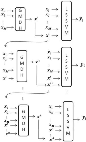
– Step 4: The GLSSVM algorithm is carried out by re-peating steps 2 to 4 untilk= 5 iterations. The GLSSVM model with the minimum value of the RMSE is selected as the output model. The configuration of the GLSSVM structure is shown in Fig. 4.
3 Case study
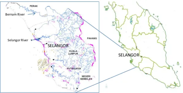
In this study, monthly flow data from Selangor and Bernam rivers in Selangor, Malaysia have been selected as the study sites. The location of these rivers are shown in Fig. 5. Bernam river is located between the Malaysian states of Perak and Selangor, demarcating the border of the two states whereas Selangor river is a major river in Selangor, Malaysia. The latter runs from Kuala Kubu Bharu in the east and con-verges into the Straits of Malacca at Kuala Selangor in the west.
The catchment area at Selangor site (3.24◦, 101.26◦) is 1450 km2and the mean elevation is 8 m whereas the catch-ment area at Bernam site (3.48◦, 101.21◦) is 1090 km2with the mean elevation is 19 m. Both these rivers basins have sig-nificant effects on the drinking water supply, irrigation and aquaculture activities such as the cultivation of fresh water fishes for human consumption.
The periods of the observed data are 47 years (564 months) with an observation period between January 1962 and De-cember 2008 for Selangor river and 43 years (516 months) from January 1966 to December 2008 for Bernam river. The training dataset of 504 monthly records (Jan. 1962 to Dis. 2004) for Selangor river and 456 monthly records (Jan. 1966 to Dis. 2004) was used to train the network to obtain parameters model. Another dataset consisting of 60 monthly (Jan. 2005 to Dis. 2008) records was used as test-ing dataset for both stations (Fig. 6).
Before starting the training, the collected data were nor-malized within the range of 0 to 1 by using the following formula:
xt = 0.1 + yt
1.2 max(yt)
(19) wherextis the normalized value,yt is the actual value and
max(yt)is the maximum value in the collected data.
The performances of each model for both training and forecasting data are evaluated according to the root-mean-square error (RMSE) and correlation coefficient (R) which
Fig. 4.The structure of the GLSSVM.
are widely used for evaluating results of time series forecast-ing. The RMSE andRare defined as:
RMSE =
v u u t 1
n n X
t=1
(yi −oi)2 (20)
R =
1
n Pn
i=1 (yi − ¯y) (oi − ¯o) q
1
n Pn
i=1 (yi − ¯y)2 q
1
n Pn
i=1 (oi − ¯o)
(21)
whereoiandyiare the observed and forecasted values at data
Fig. 5.Location of the study sites.
4 Result and discussion
4.1 Fitting the ARIMA models to the data
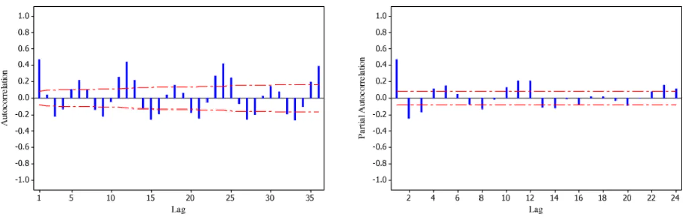
The sample autocorrelation function (ACF) and partial auto-correlation function (PACF) for Selangor and Bernam river series are plotted in Figs. 7 and 8 respectively. The ACFs curve of the monthly flow data of these rivers decayed with mixture of sine wave pattern and exponential curve that re-flects the random periodicity of the data and indicates the need for seasonal MA terms in the model. For PACF, there were significant lags at spikes from lag 1 to 5, which suggest an AR process. In the PACF, there were significant spikes present near lags 12 and 24, and therefore the series would be needed for seasonal AR process. The identification of best model for river flow series is based on minimum AIC as shown in Table 1. The criteria to judge the best model based on AIC show that ARIMA(1, 0, 0)×(1, 0, 1)12 was selected as the best model for Selangor river and the ARIMA (2, 0, 0)×(2, 0, 2)12 would be relatively the best model for Bernam river.
Since the ARIMA (1, 0, 0)×(1, 0, 1)12 is the best model for Selangor river and ARIMA (2, 0, 0)×(2, 0, 2)12 for Bernam river, then the model is used to identify the input structures. The ARIMA (2, 0, 0)×(2, 0, 2)12model can be written as:
1 −0.3515B −0.1351B2 1−0.7014B12 −0.2933B24
xt =
1 −0.5802B12 −0.3720B24at xt = 0.3515xt−1 +0.1351xt−2+0.7014xt−12
−0.2465xt−13 −0.0948xt−14 +0.2933xt−24
Table 1. Comparison of ARIMA models’ Statistical Results for Selangor and Bernam rivers.
Selangor River Bernam River
ARIMA Model AIC ARIMA Model AIC
(1, 0, 0)×(1, 0, 1)12 −4.765 (1, 0, 0)×(1, 0, 1)12 −4.458 (1, 0, 0)×(3, 0, 0)12 −4.620 (5, 0, 0)×(2, 0, 2)12 −4.251 (1, 0, 0)×(1, 0, 0)12 −4.514 (3, 0, 0)×(2, 0, 1)12 −4.459 (1, 0, 1)×(3, 0, 0)12 −4.614 (2, 0, 0)×(1, 0, 1)12 −4.466 (1, 0, 1)×(1, 0, 1)12 −4.757 (2,0,0)×(2,0,2)12 −4.467
−0.1031xt−25 −0.0396xt−26 −0.5802at−12
−0.3720at−24 +at
and the ARIMA (1, 0, 0)×(1, 0, 1)12 model can be written as:
(1 −0.4013B)1 −0.9956B12xt = (1 −0.9460B) at xt = 0.4013xt−1 +0.9956xt−12
−0.3995xt−13 −0.9460at−12 +at
The above equation for Selangor river can be rewritten as:
xt =f (xt−1, xt−12, xt−13, at−12) (22)
and for Bernam river as:
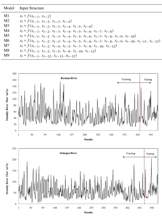
Table 2.The Input Structure of the Models for Forecasting of Selangor River Flow.
Model Input Structure M1 xt=f (xt−1, xt−2)
M2 xt=f (xt−1, xt−2, xt−3, xt−4)
M3 xt=f (xt−1, xt−2, xt−3, xt−4, xt−5, xt−6)
M4 xt=f (xt−1, xt−2, xt−3, xt−4, xt−5, xt−6, xt−7, xt−8)
M5 xt=f (xt−1, xt−2, xt−3, xt−4, xt−5, xt−6, xt−7, xt−8, xt−9, xt−10)
M6 xt=f (xt−1, xt−2, xt−3, xt−4, xt−5, xt−6, xt−7, xt−8, xt−9, xt−10, xt−11, xt−12)
M7 xt=f (xt−1, xt−2, xt−4, xt−5, xt−7, xt−9, xt−10, xt−12)
M8 xt=f (xt−1, xt−2, xt−5, xt−8, xt−10, xt−12)
M9 xt=f (xt−1, xt−12, xt−13, at−12)
Fig. 6.Time series of monthly river flow of Selangor and Bernam rivers.
4.2 Fitting ANN to the data
One of the most important steps in developing a satisfactory forecasting model such as ANN and LSSVM models is the selection of the input variables. In this study, the nine input structures which having various input variables are trained and tested by LSSVM and ANN. Four approaches were used to identify the input structures. The first approach, six model inputs were chosen based on the past river flow. The appro-priate lags were chosen by setting the input layer nodes equal
to the number of the lagged variables from river flow data,
xt−1, xt−2, ..., xt−p wherep is 2, 4, 6, 8, 10 and 12. The
second, third and forth approaches were identified using cor-relation analysis, stepwise regression analysis and ARIMA model, respectively. The model input structures of these forecasting models are shown in Tables 2 and 3.
Table 3.The Input Structure of the Models for Forecasting of Bernam River Flow.
Model Input Structure M1 xt=f (xt−1, xt−2)
M2 xt=f (xt−1, xt−2, xt−3, xt−4)
M3 xt = f (xt−1, xt−2, xt−3, xt−4, xt−5, xt−6)
M4 xt=f (xt−1, xt−2, xt−3, xt−4, xt−5, xt−6, xt−7, xt−8)
M5 xt=f (xt−1, xt−2, xt−3, xt−4, xt−5, xt−6, xt−7, xt−8, xt−9, xt−10)
M6 xt=f (xt−1, xt−2, xt−3, xt−4, xt−5, xt−6, xt−7, xt−8, xt−9, xt−10, xt−11, xt−12)
M7 xt=f (xt−1, xt−2, xt−4, xt−5, xt−6, xt−7, xt−8, xt−10, xt−11, xt−12)
M8 xt=f (xt−1, xt−2, xt−4, xt−5, xt−7, xt−10, xt−12)
M9 xt=f (xt−1, xt−2, xt−12, xt−13, xt−14, xt−24, xt−25, xt−26, at−12, at−24)
Fig. 7.The autocorrelation and partial autocorrelation of river flow series of Selangor River.
Fig. 8.The autocorrelation and partial autocorrelation of river flow series of Bernam river.
to the hidden layer, the hyperbolic tangent sigmoid transfer function commonly used in hydrology was applied. From the hidden layer to the output layer, a linear function was employed as the transfer function because the linear function is known to be robust for a continuous output variable.
The network was trained for 5000 epochs using the con-jugate gradient descent back-propagation algorithm with a learning rate of 0.001 and a momentum coefficient of 0.9. The nine models (M1–M9) having various input structures
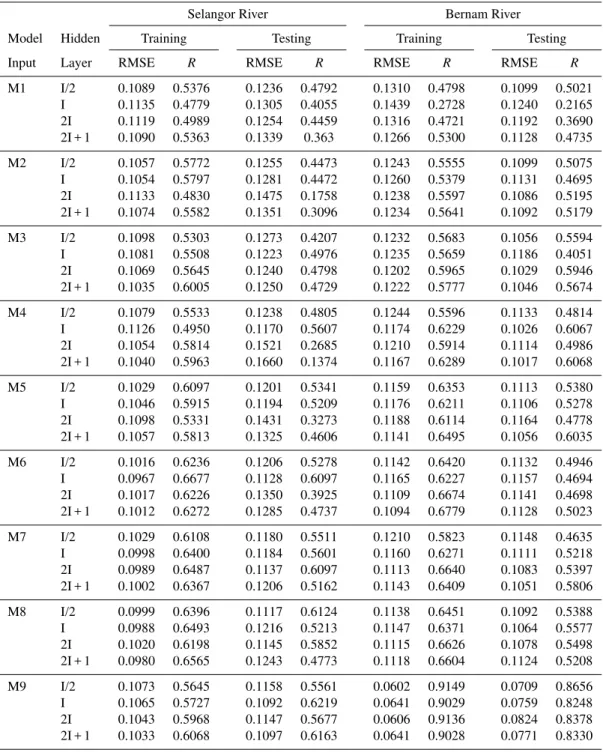
Table 4.Comparison of ANN structures for Selangor and Bernam River.
Selangor River Bernam River Model Hidden Training Testing Training Testing Input Layer RMSE R RMSE R RMSE R RMSE R
M1 I/2 0.1089 0.5376 0.1236 0.4792 0.1310 0.4798 0.1099 0.5021 I 0.1135 0.4779 0.1305 0.4055 0.1439 0.2728 0.1240 0.2165 2I 0.1119 0.4989 0.1254 0.4459 0.1316 0.4721 0.1192 0.3690 2I + 1 0.1090 0.5363 0.1339 0.363 0.1266 0.5300 0.1128 0.4735 M2 I/2 0.1057 0.5772 0.1255 0.4473 0.1243 0.5555 0.1099 0.5075 I 0.1054 0.5797 0.1281 0.4472 0.1260 0.5379 0.1131 0.4695 2I 0.1133 0.4830 0.1475 0.1758 0.1238 0.5597 0.1086 0.5195 2I + 1 0.1074 0.5582 0.1351 0.3096 0.1234 0.5641 0.1092 0.5179 M3 I/2 0.1098 0.5303 0.1273 0.4207 0.1232 0.5683 0.1056 0.5594 I 0.1081 0.5508 0.1223 0.4976 0.1235 0.5659 0.1186 0.4051 2I 0.1069 0.5645 0.1240 0.4798 0.1202 0.5965 0.1029 0.5946 2I + 1 0.1035 0.6005 0.1250 0.4729 0.1222 0.5777 0.1046 0.5674 M4 I/2 0.1079 0.5533 0.1238 0.4805 0.1244 0.5596 0.1133 0.4814 I 0.1126 0.4950 0.1170 0.5607 0.1174 0.6229 0.1026 0.6067 2I 0.1054 0.5814 0.1521 0.2685 0.1210 0.5914 0.1114 0.4986 2I + 1 0.1040 0.5963 0.1660 0.1374 0.1167 0.6289 0.1017 0.6068 M5 I/2 0.1029 0.6097 0.1201 0.5341 0.1159 0.6353 0.1113 0.5380 I 0.1046 0.5915 0.1194 0.5209 0.1176 0.6211 0.1106 0.5278 2I 0.1098 0.5331 0.1431 0.3273 0.1188 0.6114 0.1164 0.4778 2I + 1 0.1057 0.5813 0.1325 0.4606 0.1141 0.6495 0.1056 0.6035 M6 I/2 0.1016 0.6236 0.1206 0.5278 0.1142 0.6420 0.1132 0.4946 I 0.0967 0.6677 0.1128 0.6097 0.1165 0.6227 0.1157 0.4694 2I 0.1017 0.6226 0.1350 0.3925 0.1109 0.6674 0.1141 0.4698 2I + 1 0.1012 0.6272 0.1285 0.4737 0.1094 0.6779 0.1128 0.5023 M7 I/2 0.1029 0.6108 0.1180 0.5511 0.1210 0.5823 0.1148 0.4635 I 0.0998 0.6400 0.1184 0.5601 0.1160 0.6271 0.1111 0.5218 2I 0.0989 0.6487 0.1137 0.6097 0.1113 0.6640 0.1083 0.5397 2I + 1 0.1002 0.6367 0.1206 0.5162 0.1143 0.6409 0.1051 0.5806 M8 I/2 0.0999 0.6396 0.1117 0.6124 0.1138 0.6451 0.1092 0.5388 I 0.0988 0.6493 0.1216 0.5213 0.1147 0.6371 0.1064 0.5577 2I 0.1020 0.6198 0.1145 0.5852 0.1115 0.6626 0.1078 0.5498 2I + 1 0.0980 0.6565 0.1243 0.4773 0.1118 0.6604 0.1124 0.5208 M9 I/2 0.1073 0.5645 0.1158 0.5561 0.0602 0.9149 0.0709 0.8656 I 0.1065 0.5727 0.1092 0.6219 0.0641 0.9029 0.0759 0.8248 2I 0.1043 0.5968 0.1147 0.5677 0.0606 0.9136 0.0824 0.8378 2I + 1 0.1033 0.6068 0.1097 0.6163 0.0641 0.9028 0.0771 0.8330
Table 4 shows the performance of ANN varying with the number of neurons in the hidden layer.
In the training phase for Selangor river, the M6 model with the number of hidden neurons I obtained the best RMSE andR statistics of 0.0967 and 0.6677, respectively. While in testing phase, the M9 model with 2I + 1 numbers of hid-den neurons had the best RMSE andR statistics of 0.1097 and 0.6163, respectively.
On the other hand, for the Bernam river, the M9 model with the number of hidden neurons was I/2 obtained the best RMSE andRstatistics, in the training and testing phase.
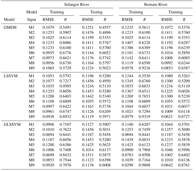
Table 5.The RMSE andRstatistics of GMDH, LSSVM and GLSSVM Models for Selangor and Bernam River. Selangor River Bernam River Model Training Testing Training Training Model Input RMSE R RMSE R RMSE R RMSE R
GMDH M1 0.1079 0.5491 0.1251 0.4557 0.1235 0.5611 0.1072 0.5376 M2 0.1253 0.5907 0.1476 0.4896 0.1233 0.6100 0.1411 0.5760 M3 0.1025 0.6114 0.1199 0.5353 0.1025 0.6114 0.1199 0.5353 M4 0.1233 0.6086 0.1411 0.5767 0.1407 0.6228 0.1192 0.6287 M5 0.1233 0.6100 0.1411 0.5760 0.1386 0.6389 0.1196 0.6239 M6 0.0955 0.6776 0.1144 0.6052 0.1101 0.6733 0.1034 0.5850 M7 0.0973 0.6621 0.1176 0.5742 0.1142 0.6411 0.1008 0.6085 M8 0.0956 0.6750 0.1164 0.5797 0.1119 0.6598 0.0992 0.6244 M9 0.1065 0.5729 0.1224 0.5023 0.0578 0.9216 0.0853 0.8387 LSSVM M1 0.1053 0.5792 0.1196 0.5280 0.1244 0.5530 0.1080 0.5263 M2 0.1077 0.7217 0.1456 0.4950 0.1345 0.6760 0.1300 0.5209 M3 0.1035 0.0505 0.1216 0.5110 0.1035 0.6033 0.1216 0.5110 M4 0.1253 0.6056 0.1453 0.5280 0.1367 0.6511 0.1225 0.6026 M5 0.1208 0.6403 0.1442 0.5340 0.1269 0.7653 0.1300 0.5230 M6 0.1108 0.6809 0.1055 0.5572 0.1108 0.6809 0.1055 0.5572 M7 0.0997 0.6422 0.1163 0.5738 0.1044 0.6037 0.1031 0.6037 M8 0.0961 0.6747 0.1126 0.6269 0.1021 0.7294 0.1009 0.6118 M9 0.0938 0.6932 0.1119 0.5971 0.0579 0.9319 0.0621 0.8727 GLSSVM M1 0.0908 0.7107 0.1127 0.5907 0.1180 0.6207 0.1044 0.5701 M2 0.1010 0.7622 0.1456 0.5031 0.1253 0.7459 0.1257 0.5690 M3 0.0694 0.8441 0.1187 0.5458 0.0694 0.8441 0.1187 0.5458 M4 0.1187 0.6056 0.1453 0.5280 0.1439 0.6033 0.1233 0.5878 M5 0.1200 0.6386 0.1425 0.5625 0.1425 0.6123 0.1237 0.5839 M6 0.1006 0.7408 0.1014 0.6137 0.0900 0.7968 0.1046 0.5996 M7 0.0698 0.8432 0.1511 0.5875 0.0783 0.8508 0.1002 0.6402 M8 0.0853 0.7544 0.1123 0.6398 0.1039 0.7164 0.1010 0.6136 M9 0.0920 0.7076 0.1138 0.6008 0.0290 0.9808 0.0642 0.8761
4.3 Fitting LSSVM to the data
The selection of appropriate input data sets is an important consideration in the LSSVM modelling. In the training and testing of the LSSVM model, the same input structures of the data set (M1–M9) have been used. The precision and conver-gence of LSSVM was affected by (γ , σ2). There is no struc-tured way to choose the optimal parameters of LSSVM. In order to obtain the optimal model parameters of the LSSVM, a grid search algorithm was employed in the parameter space. In order to evaluate the performance of the proposed ap-proach, a grid search of (γ , σ2) withγ in the range 10 to 1000 andσ2in the range 0.01 to 1.0 was considered. For each hyperparameter pair (γ σ2)in the search space, a 5-fold cross validation on the training set is performed to pre-dict the prepre-diction error. The best fit model structure for each model is determined according to criteria of the per-formance evaluation. In the study, the LSSVM model was implemented with the software package LS-SVMlab1.5 (Pel-ckmans et al., 2003). As the LSSVM method is employed, a
kernel function has to be selected from the qualified function. Previous works on the use of LSSVM in time series model-ing and forecastmodel-ing have demonstrated that RBF performs favourably (Liu and Wang, 2008; Yu et al., 2006; Gencoglu and Ulyar, 2009). Therefore, the RBF, which has a parame-terγ as in Eq. (14), is adopted in this work. Table 5 shows the results of the performance obtained during in the training and testing period of the LSSVM approach.
As seen in Table 5, the LSSVM models are evaluated based on their performances in the training and testing sets. For the training phase of Selangor river, the best value of the RMSE andR statistics are 0.0938 and 0.6932 (in M9), respectively. However, during the testing phase, the lowest value of the RMSE was 0.1055 (in M6) and the highest value of the R was 0.6269 (in M8). On the other hand, for the Bernam river, the M9 model obtained the best RMSE andR
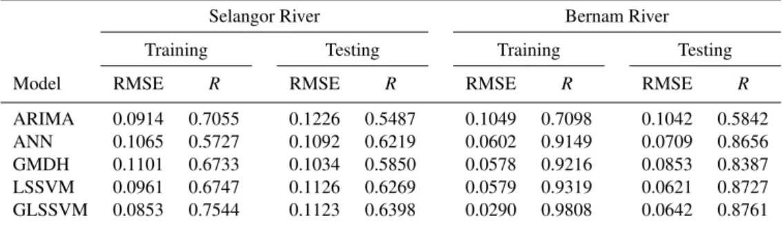
Table 6.Forecasting performance indices of models for Selangor and Bernam River.
Selangor River Bernam River Training Testing Training Testing Model RMSE R RMSE R RMSE R RMSE R
ARIMA 0.0914 0.7055 0.1226 0.5487 0.1049 0.7098 0.1042 0.5842 ANN 0.1065 0.5727 0.1092 0.6219 0.0602 0.9149 0.0709 0.8656 GMDH 0.1101 0.6733 0.1034 0.5850 0.0578 0.9216 0.0853 0.8387 LSSVM 0.0961 0.6747 0.1126 0.6269 0.0579 0.9319 0.0621 0.8727 GLSSVM 0.0853 0.7544 0.1123 0.6398 0.0290 0.9808 0.0642 0.8761
4.4 Fitting GMDH and GLSSVM with the data
In designing the GMDH and GLSSVM models, one must de-termine the following variables: the number of input nodes and layers. The selection of the number of input that corre-sponds to the number of variables plays an important role in many successful applications of GMDH.
GMDH works by building successive layers with complex connections that are created by using second-order polyno-mial function. The first layer created is made by comput-ing regressions of the input variables followed by the second layer that is created by computing regressions of the output value. Only the best variables are chosen from each layer and this process continues until the pre-specified selection crite-rion is found.
The proposed hybrid learning architecture is composed of two stages. In the first stage, GMDH is used to determine the useful inputs for LSSVM method. The estimated output val-uesx′is used as the feedback value which is combined with the input variables{x1, x2, ... ,xM}in the next loop
calcu-lations. The second stage, the LSSVM mapping the combi-nation inputs variables{x1, x2, ..., xM, x′}are used to seek
optimal solutions for determining the best output for fore-casting. To make the GMDH and GLSSVM models simple and reduce some of the computational burden, only nine in-put nodes (M1–M9) and five hidden layers (k) from 1 to 5 have been selected for this experiment.
In the LSSVM model, the parameter values forγ andσ2
need to be first specified at the beginning. Then, the parame-ters of the model are selected by grid searching withγwithin the range of 10 to 1000 andσ2within the range of 0.01 to 1.0. For each parameter pair (γ , σ2) in the search space, 5-fold cross validation of the training set is performed to predict the prediction error. The performances of GMDH and GLSSVM for time series forecasting models are given in Table 5.
For Selangor river, in the training and testing phase, the best value of the RMSE andR statistics for GMDH model were obtained using M6. In the training phase, GLSSVM model obtained the best RMSE and R statistics of 0.0694 and 0.8441 (in M3) respectively. While in testing phase,
the lowest value of the RMSE was 0.1014 (in M6) and the highest value of theR was 0.6398 (in M8). However, in the training and testing phase for Bernam river, the best value of RMSE andRfor LSSM, GMDH and GLSSVM models were obtained by using M9.
The model that performs best during testing is chosen as the final model for forecasting the sixty monthly flows. As seen in Table 5, for Selangor river, the model input M8 gave the best performance for LSSVM and GLSSVM mod-els, and M6 for the GMDH model. On the other hand, for Bernam river, the model input M9 gave the best performance for LSSVM, GMDH and GLSSVM models and hence, these model inputs have been chosen as the final input structures models
4.5 Comparisons of forecasting models
To analyse these models further, the error statistics of the optimum ARIMA, ANN, GMDH, LSSVM and GLSSVM ar compared. The performances of all the models for training and testing data set are in Table 6.
Comparing the performances of ARIMA, ANN, GMDH, LSSVM and GLSSVM models for in training of Selangor and Bernam rivers, the lowest RMSE and the largest R were calculated for GLSSVM model respectively. For test-ing data, the best value of RMSE and R were found for GLSSVM model. However, the lowest RMSE were observed for GMDH model for Selangor river and LSSVM model for Bernam river. From the Table 6, it is evident that the GLSSVM performed better than the ARIMA, ANN, GMDH and LSSVM models in the training and testing process.
GLSSVM is slightly superior to the other models. The re-sults obtained in this study indicate that the GLSSVM model is a powerful tool to model the river flow time series and can provide a better prediction performance as compared to the ARIMA, ANN, GMDH and LSSVM time series ap-proach. The results indicate that the best performance can be obtained by the GLSSVM model and this is followed by LSSVM, GMDH, ANN and ARIMA models.
5 Conclusions
Monthly river flow estimation is vital in hydrological prac-tices. There are plenty of models used to predict river flows. In this paper, we have demonstrated how the monthly river flow could be represented by a hybrid model combining the GMDH and LSSVM models. To illustrate the capability of the LSSVM model, Selangor and Bernam rivers, located in Selangor of Peninsular Malaysia were chosen as the case study. The river flow forecasting models having various input structures were trained and tested to investigate the applica-bility of GLSSVM compared with ARIMA, ANN, GMDH and LSSVM models. One of the most important issues in developing a satisfactory forecasting model such as ANN, GMDH, LSSVM and GLSSVM models is the selection of the input variables. Empirical results on the two data sets using five different models have clearly revealed the effi-ciency of the hybrid model. By using a evaluation of per-formance test, the input structure based on ARIMA model is decided as the optimal input factor. In terms of RMSE andRvalues taken from both data sets, the hybrid model has the best in training. In testing, high correlation coefficient (R) was achieved by using the hybrid model for both data sets. However, the lowest value of RMSE were achieved us-ing the GMDH for Selangor river and LSSVM for Bernam river. These results show that the hybrid model provides a robust modeling capable of capturing the nonlinear nature of the complex river flow time series and thus producing more accurate forecasts.
Acknowledgements. The authors would like to thank the Ministry of Science, Technology and Innovation (MOSTI), Malaysia for funding this research with grant number 79346 and Department of Irrigation and Drainage Malaysia for providing the data of river flow.
Edited by: E. Todini
References
Abraham, A. and Nath, B.: A neuro-fuzzy approach for modeling electricity demand in Victoria, Appl. Soft Comput., 1(2), 127– 138, 2001.
Adamowski, J. and Sun, K.: Development of a coupled wavelet transform and neural network method for flow forecasting of non-perennial rivers in semi-arid watersheds, J. Hydrol., 390(1– 2), 85–91, 2010.
Affandi, A. K. and Watanabe, K.: Daily groundwater level fluctua-tion forecasting using soft computing technique, Nat. Sci., 5(2), 1–10, 2007.
Afshin, M., Sadeghian, A. and Raahemifar, K.: On efficient tuning of LS-SVM hyper-parameters in short-term load forecasting: A comparative study, Proc. of the 2007 IEEE Power Engineering Society General Meeting (IEEE-PES), 2007.
Akaike, H.: A new look at the statistical model identification, IEEE T. Automat. Contr., 19, 716–723, 1974.
Akhtar, M. K., Corzo, G. A., van Andel, S. J., and Jonoski, A.: River flow forecasting with artificial neural networks using satel-lite observed precipitation pre-processed with flow length and travel time information: case study of the Ganges river basin, Hydrol. Earth Syst. Sci., 13, 1607–1618, doi:10.5194/hess-13-1607-2009, 2009.
ASCE Task Committee on Application of Artificial Neural Net-works in Hydrology: Artificial neural netNet-works in hydrology, II – Hydrologic applications, J. Hydrol. Eng., 5(2), 124–137, 2000. Asefa, T., Kemblowski, M., McKee, M., and Khalil, A.: Multi-time scale stream flow prediction: The support vector machines approach, J. Hydrol., 318, 7–16, 2006.
Atiya, A. F., El-Shoura, S. M., Shaheen, S. I., and El-Sherif, M. S.: A Comparison between neural-network forecasting techniques-Case Study: River flow forecasting, IEEE T. Neural Netw., 10(2), 402–409, 1999.
Birkinshaw, S. J., Parkin, G., and Rao, Z.: A hybrid neural networks and numerical models approach for predicting groundwater ab-straction impacts, J. Hydroinform., 10.2, 127–137, 2008. Box, G. E. P. and Jenkins, G.: Time Series Analysis, Forecasting
and Control, Holden-Day, San Francisco, CA, 1970.
Brockwell, P. J. and Davis, R. A.: Introduction to Time Series and Forecasting, Springer, Berlin, 2002.
Camastra, F. and Colla, A.: Mneural short-term rediction based on dynamics reconstruction, ACM – Association of Computing Ma-chinery, 9(1), 45–52, 1999.
Chang, F. J. and Hwang, Y. Y.: A self-organization algorithm for real-time flood forecast, Hydrol. Process., 13, 123–138, 1999. Chen, K. Y. and Wang, C. H.: A hybrid ARIMA and support vector
machines in forecasting the production values of the machinery industry in Taiwan, Expert Syst. Appl., 32, 254–264, 2007. Coulibaly, P. and Evora, N. D.: Comparison of neural network
methods for infilling missing daily weather records, J. Hydrol., 341, 27–41, 2007.
de Vos, N. J. and Rientjes, T. H. M.: Constraints of artificial neural networks for rainfall-runoff modelling: trade-offs in hydrological state representation and model evaluation, Hydrol. Earth Syst. Sci., 9, 111–126, doi:10.5194/hess-9-111-2005, 2005.
Dolling, O. R. and Varas, E. A.: Artificial neural networks for streamflow prediction, J. Hydraul. Res., 40(5), 547–554, 2003. Fernandez, C. and Vega, J. A.: Streamflow drought time series
fore-casting: a case study in a small watershed in north west spain, Stoch. Environ. Res. Risk Assess., 23, 1063–1070, 2009. Firat, M.: Comparison of Artificial Intelligence Techniques for
river flow forecasting, Hydrol. Earth Syst. Sci., 12, 123–139, doi:10.5194/hess-12-123-2008, 2008.
Firat, M. and Gungor, M.: River flow estimation using adaptive neuro fuzzy inference system, Math. Comput. Simulat., 75(3–4), 87–96, 2007.
Firat, M. and Turan, M. E.: Monthly river flow forecasting by an adaptive neuro-fuzzy inference system, Water Environ. J., 24, 116–125, 2010.
Gencoglu, M. T. and Uyar, M.: Prediction of flashover voltage of insulators using least squares support vector machines, Expert Syst. Appl., 36, 10789–10798, 2009.
Gestel, T. V., Suykens, J. A. K., Baestaens, D. E., Lambrechts, A., Lanckriet, G., Vandaele, B., Moor, B. D., and Vandewalle, J.: Fi-nancial time series prediction using Least Squares Support Vec-tor Machines within the evidence framework, IEEE T. Neural Netw., 12(4), 809–821, 2001.
Han, M. and Wang, M.: Analysis and modeling of multivariate chaotic time series based on neural network, Expert Syst. Appl., 2(36), 1280–1290, 2009.
Hsu, K. L., Gupta, H. V., and Sorooshian, S.: Artificial neural net-work modeling of the rainfall runoff process, Water Resour. Res., 31(10), 2517–2530, 1995.
Huang, W., Bing Xu, B., and Hilton, A.: Forecasting flow in apalachicola river using neural networks, Hydrol. Process., 18, 2545–2564, 2004.
Hung, N. Q., Babel, M. S., Weesakul, S., and Tripathi, N. K.: An artificial neural network model for rainfall forecasting in Bangkok, Thailand, Hydrol. Earth Syst. Sci., 13, 1413–1425, doi:10.5194/hess-13-1413-2009, 2009.
Ivanenko, A. G.: Polynomial theory of complex system, IEEE Trans. Syst., Man Cybern. SMCI-1, No. 1, 364–378, 1971. Ivakheneko A. G. and Ivakheneko, G. A.: A review of problems
solved by algorithms of the GMDH, S. Mach. Perc., 5(4), 527– 535, 1995.
Jain, A. and Kumar, A.: An evaluation of artificial neural network technique for the determination of infiltration model parameters, Appl. Soft Comput., 6, 272–282, 2006.
Jain, A. and Kumar, A. M.: Hybrid neural network models for hy-drologic time series forecasting, Appl. Soft Comput., 7, 585– 592, 2007.
Kang, S.: An Investigation of the Use of Feedforward Neural Net-work for Forecasting, Ph.D. Thesis, Kent State University, 1991. Karunasinghe, D. S. K. and Liong, S. Y.: Chaotic time series pre-diction with a global model: Artificial neural network, J. Hydrol., 323, 92–105, 2006.
Keskin, M. E. and Taylan, D.: Artifical models for interbasin flow prediction in southern turkey, J. Hydrol. Eng., 14(7), 752–758, 2009.
Kisi, O.: River flow modeling using artificial neural networks, J. Hydrol. Eng., 9(1), 60–63, 2004.
Kisi, O.: River flow forecasting and estimation using different arti-ficial neural network technique, Hydrol. Res., 39.1, 27–40, 2008.
Kisi, O.: Wavelet regression model as an alternative to neural net-works for monthly streamflow forecasting, Hydrol. Process., 23, 3583–3597, 2009.
Lin, C. J., Hong, S. J., and Lee, C. Y.: Using least squares support vector machines for adaptive communication channel equaliza-tion, Int. J. Appl. Sci. Eng., 3(1), 51–59, 2005.
Lin, J. Y., Cheng, C. T., and Chau, K. W.: Using support vector machines for long-term discharge prediction, Hydrolog. Sci. J., 51(4), 599–612, 2006.
Liong, S.Y. and Sivapragasam, C.: Flood stage forecasting with support vector machines, J. Am. Water Resour. Assoc., 38(1), 173–196, 2002.
Lippmann, R. P.: An introduction to computing with neural nets, IEEE ASSP Magazine, April, 4–22, 1987.
Liu, L. and Wang, W.: Exchange Rates Forecasting with Least Squares Support Vector Machine, Proc. of the IEEE 2008 In-ternational Conference on Computer Science and Software En-gineering (IEEE-CSSE), 1017–1019, 2008.
Maier, H. R. and Dandy, G. C.: Neural networks for the produc-tion and forecasting of water resource variables: a review and modelling issues and application, Environ. Modell. Softw., 15, 101–124, 2000.
Misra, D., Oommen, T., Agarwal, A., Mishra, S. K., and Thomp-son, A. M.: Application and analysis of support vector machine based simulation for runoff and sediment yield, Biosyst. Eng., 103, 527–535, 2009.
Modarres, R.: Streamflow drought time series forecasting, Stoch. Environ. Res. Risk Assess., 21, 223–233, 2007.
Muhamad, J. R. and Hassan, J. N.: Khabur River flow using arti-ficial neural networks, Al Rafidain Engineering, 13(2), 33–42, 2005.
Nariman-Zadeh, N., Darvizeh, A., Felezi, M. E., and Gharababaei, H.: Polynomial modelling of explosive process of metalic pow-ders using GMDH-type neural networks and singular value de-composition, Model. Simul. Sci. Eng., 10, 727–744, 2002. Onwubolu, G. C.: Design of hybrid differential evolution and group
method of data handling networks for modeling and prediction, Information Sci., 178, 3616–3634, 2008.
Onwubolu, G. C., Buryan, P., Garimella, S., Ramachandran, V., Buadromo, V., and Abraham, A.: Self-organizing data mining for weather forecasting, IADIS European Conference Data Ming, 81–88, 2007.
Pelckmans, K., Suykens, J., Van, G., De Brabanter, J., Lukas, L., Hanmers, B., De Moor, B., and Vandewalle, J.: LS-SVMlab: a MATLAB/C toolbox for Least Square Support Vector Ma-chines; http://www.esat.kuleuven.ac.be/sista/lssvmlab (last ac-cess: 31 September 2010: toolbox updated to LS-SVMlab v1.7), 2003.
Rientjes, T. H. M.: Inverse modelling of the rainfall-runoff relation; a multi objective model calibration approach, Ph.D. thesis, Delft University of Technology, Delft, The Netherlands, 2004. Rojas, I., Valenzuela, O., Rojas, F., Guillen, A., Herrera, L. J.,
Po-mares, H., Marquez, L., and Pasadas, M.: Soft-computing tech-niques and ARMA model for time series prediction, Neurocom-puting, 71(4–6), 519–537, 2008.
See, L. and Openshaw, S.: A hybrid multi-model approach to river level forecasting, Hydrolog. Sci. J., 45(4), 523–536, 2009. Shamseldin, A. Y.: Application of Neural Network Technique to
Su, C. T., Tong, L. I., and Leou, C. M.: Combination of time se-ries and neural network for reliability forecasting modeling, J. Chinese Ind. Eng., 14, 419–429, 1997.
Sun, G. and Guo, W.: Robust mobile geo-location algorithm based on LSSVM, IEEE T. Veh. Technol., 54(2), 1037–1041, 2005. Suykens, J. A. K. and Vandewalle, J.: Least squares support vector
machine classifiers, Neural Process. Lett, 9(2), 293–300, 1999. Suykens, J. A. K., Van Gestel, T., De Brabanter, J., De Moor, B., and
Vandewalle, J.: Least squares support vector machines, World Scientific, Singapore, 2002.
Tamura, H. and Kondo, T.: Heuristic free group method of data han-dling algorithm of generating optional partial polynomials with application to air pollution prediction, Int. J. Syst. Sci., 11, 1095– 1111, 1980.
Tang, Z. and Fishwick, P. A.: Feedforward Neural Nets as Models for Time Series Forecasting, ORSA J. Comput., 5(4), 374–385, 1993.
Tay, F. and Cao, L. : Application of support vector machines in financial time series forecasting, Omega Int. J. Manage. Sci., 29(4), 309–317, 2001.
Thiessen, U. and Van Brakel, R.: Using support vector machines for time series prediction, Chemometr. Intell. Lab., 69, 35–49, 2003. Vapnik, V.: The nature of Statistical Learning Theory, Springer
Ver-lag, Berlin, 1995.
Voss, M. S. and Feng, X.: A new methodology for emergent sys-tem identification using particle swarm optimization (PSO) and the group method data handling (GMDH), GECCO 2002, 1227– 1232, 2002.
Wang, H. and Hu, D.: Comparison of SVM and LS-SVM for Re-gression, IEEE, 279–283, 2005.
Wang, W., Gelder, P. V., and Vrijling, J. K.: Improving daily stream flow forecasts by combining ARMA and ANN models, Interna-tional Conference on Innovation Advances and Implementation of Flood Forecasting Technology, 2005.
Wang, W., Gelder, V. P., and Vrijling, J. K.: Forecasting daily stream flow using hybrid ANN models, J. Hydrol., 324, 383– 399, 2006.
Wang, W. C., Chau, K. W., Cheng, C. T., and Qiu, L.: A Compar-ison of Performance of Several Artificial Intelligence Methods for Forecasting Monthly Discharge Time Series, J. Hydrol., 374, 294–306, 2009.
Wang, X., Li, L., Lockington, D., Pullar, D., and Jeng, D.S.: Self-organizing polynomial neural network for modeling complex hy-drological processes, Research Report No. R861:1-29, 2005. Wong, F. S.: Time series forecasting using backpropagation neural
network, Neurocomputing, 2, 147–159, 1991.
Wu, C. L., Chau, K. W., and Li, Y. S.: Predicting monthly streamflow using driven models coupled with data-preprocessing techniques, Water Resour. Res., 45, W08432, doi:10.1029/2007WR006737, 2009.
Yang, Q., Lincang Ju, L., Ge, S., Shi, R., and Yuanli Cai, Y.: Hy-brid fuzzy neural network control for complex industrial pro-cess, International conference on intelligent computing, Kun-ming, China, 533–538, 2006.
Yu, P. S., Chen, S. T., and Chang, I. F.: Support vector regression for real-time flood stage forecasting, J. Hydrol., 328(3–4), 704–716, 2006.
Yunrong, X. and Liangzhong, J.: Water quality prediction using LS-SVM with particle swarm optimization, Second International Workshop on Knowledge Discovery and Data Mining, 900–904, 2009.
Yurekli, K., Kurunc, A., and Simsek, H.: Prediction of Daily Streamflow Based on Stochastic Approaches, J. Spatial Hydrol., 4(2), 1–12, 2004.
Zhang, B. and Govindaraju, G.: Prediction of watershed runoff us-ing bayesian concepts and modular neural networks, Water Re-sour. Res., 36(2), 753–762, 2000.
Zhang, G., Patuwo, B. E., and Hu, M. Y.: Forecasting with artificial neural networks: the state of the art, Int. J. Forecast., 14, 35–62, 1998.
Zhang, G. P.: Time series forecasting using a hybrid ARIMA and neural network model, Neurocomputing, 50, 159–175, 2003. Zhang, G. P., Patuwo, B. E., and Hu, M. Y.: A simulation study of
artificial neural networks for nonlinear time-series forecasting, Comput. Oper. Res., 28(4), 381–396, 2001.