Modeling—Ecology, Physiology, and Cell
Biology
H. G. Othmer
F. R. Adler
M. A. Lewis
J. C. Dallon
viii + 415 p. 24 cm. Includes 179 illustrations.
Includes biographical references, author/editor index, and subject index. ISBN 0-13-574039-8
1. Mathematical modeling in ecology and evolution. 2. Mathematical modeling in physiology.
3. Mathematical modeling in cell biology. QH541.15.M3C37 1997
577/.01/5118 21 96-47909 CIP
Editorial/production supervision: ???? Manufacturing buyers: ???? and ????
c
1997 by H. G. Othmer, F. R. Adler, M. A. Lewis, and J. C. Dallon Published by Prentice-Hall, Inc.
A Simon & Shuster Company Englewood Cliffs, New Jersey 07632
All rights reserved. No part of this book may be reproduced, in any form or by any means, without permission in writing of the copyright holders.
Printed in the United States of America. 10 9 8 7 6 5 4 3 2 1
ISBN 0-13-574039-8
Prentice-Hall International (UK) Limited, London Prentice-Hall of Australia Pty. Limited, Sydney Prentice-Hall of Canada Inc., Toronto Prentice-Hall Hispanoamericana, S.A., Mexico Prentice-Hall of India Private Limited, New Delhi Prentice-Hall of Japan, Inc. Tokyo
Preface . . . . v Part I: Ecology and Evolution
Frederick R. Adler . . . . 1 1. You Bet Your Life: Life-History Strategies in Fluctuating Environments
Stephen P. Ellner . . . . 3 2. The Evolution of Species’ Niches: A Population Dynamic Perspective
Robert D. Holt and Richard Gomulkiewicz . . . . 25 3. Reflections on Models of Epidemics Triggered by the Case of Phocine
Distemper Virus among Seals
Odo Diekmann . . . . 51 4. Simple Representations of Biomass Dynamics in Structured Populations
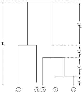
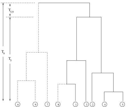
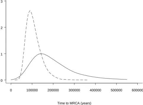
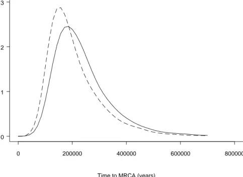
R. M. Nisbet, E. McCauley, W. S. C. Gurney, W. W. Murdoch, and A. M. de Roos . . . . 61 5. Ancestral Inference from DNA Sequence Data
Simon Tavar´e . . . . 81 Part II: Cell Biology
Mark A. Lewis . . . . 97 6. Signal Transduction and Second Messenger Systems
Hans G. Othmer . . . . 101 7. The Eukaryotic Cell Cycle: Molecules, Mechanisms, and Mathematical
Models
John J. Tyson, Kathy Chen and Bela Novak . . . . 129 8. Mathematical Models of Hematopoietic Cell Replication and Control
Michael C. Mackey . . . . 151 9. Oscillations and Multistability in Delayed Feedback Control
John Milton and Jennifer Foss . . . . 183 10. Calcium and Membrane Potential Oscillations in Pancreaticβ-Cells
Arthur Sherman . . . . 203 Part III: Physiology
Hans G. Othmer . . . . 223
Edward Pate . . . . 225
12. The Topology of Phase Resetting and the Entrainment of Limit Cycles Leon Glass . . . . 259
13. Modeling the Interaction of Cardiac Muscle with Strong Electric Fields Wanda Krassowska . . . . 281
14. Fluid Dynamics of the Heart and its Valves Charles S. Peskin and David M. McQueen . . . . 313
15. Bioconvection N. A. Hill . . . . 343
A. Age-structured Models Frederick R. Adler . . . . 357
B. Qualitative Theory of Ordinary Differential Equations Mark A. Lewis and Hans G. Othmer . . . . 361
C. An Introduction to Partial Differential Equations Hans G. Othmer . . . . 385
Author/Editor Index . . . . 391
Subject Index . . . . 403
List of Contributors . . . . 411
Colophon . . . . 415
As its name indicates, the field of mathematical biology is inherently interdis-ciplinary. Students and researchers seeking to enter this field, or to broaden their knowledge, face special challenges. How does one strike an appropriate balance between learning the details of the underlying biology and the intri-cacies of the mathematics? Are explorers in this area beset, like Odysseus, by the twin dangers of Scylla and Charybdis? Or are they at risk of being seduced by the sirens of biological complexity and mathematical elegance?
Books that seek to introduce this field must guide readers along a safe path between the same dangers. This volume finds the path not by following some pedagogical theory or by believing rumors about past shipwrecks, but by tracing the wake of successful researchers who have survived to tell the tale. Each scientist who has addressed biological questions with mathemati-cal methods has found a different way, and this book presents this diversity. The case studies presented herein invite readers to join a researcher as he or she attacks a significant biological problem from start to finish. Each chap-ter combines the focus on cutting-edge research characchap-teristic of the profes-sional literature with the emphasis on teaching characteristic of a textbook. The authors provide a synthetic view of the biological problem, illustrating the multiple approaches attempted, and the strengths and weaknesses of each. The goal is to motivate and explain biological problems and their mathemat-ical solution, while simultaneously exemplifying the process of developing a successful research program.
These case studies guide advanced undergraduates, beginning grad-uate students, and researchers along several such paths. Students who have worked to build mathematical skills will able to set sail in quest of important problems. The goal is to initiate them into both the diversity of approaches to mathematical biology and the breadth of the field. This book thus has two unique features, summarized as case studies in mathematical biology.
As a guide to both student and teacher, we suggest that the chapters can be read with the following general framework for modeling in mind.
1. The first step is to identify a biologically interesting problem which has a significant aspect that requires mathematical modeling, to identify crit-ical observations on which to base a model, and to distinguish between dependable and undependable experimental results.
2. The second step is to formulate the model conceptually, making rea-soned judgments regarding which processes to include and which to ex-clude.
3. The next step is to convert the conceptual model into a mathematical model and estimate parameters in the model, keeping in mind differing levels of certainty regarding their values.
numerically, if analytical solution is impossible, and use the results to interpret the original critical observations, make new predictions and propose new experiments.
This complex process cannot be distilled into an algorithm, because it is as much art as science. As in the experimental sciences, the techniques of mod-eling are learned by example and by hands-on experience. This book aims to provide both.
Coverage
Powerful new techniques in molecular biology, physiology, genetics and ecology are making biology more quantitative and more unified. Mathe-matical methods are needed both to analyze increasing volumes of data, and to forge connections between data shedding light on common problems from different angles.
Due to the expanding role of mathematics as a unifying force in biol-ogy, broad coverage of the field of biology is essential. The topics chosen in this volume fall into three overlapping categories: ecology, cell biology, and physiology. Although the areas have their characteristic concerns, each area uses mathematics to link levels of biological organization, depends on related mathematical techniques from dynamical systems, and, more broadly, empha-sizes that mechanisms which act at the cellular or molecular level manifest themselves in the functioning of the whole organism in its environment. Each of the three sections of the book begins with an introduction by the editors that elucidates specific themes and concerns characteristic of that section.
How to use this book
We envision three primary uses for this book: as a supplementary text to accompany a mathematical biology course, as a primary text for an intensive mathematical modeling course, and as a reference volume for researchers and students.
The mathematical level of the book is graded, becoming more ad-vanced in the later chapters. Every chapter requires that students be famil-iar and comfortable with differential equations and linear algebra (short ap-pendices outlines relevant aspects of these techniques). Partial differential equations and functional differential equations are used more and more in the later chapters, and previous background or concurrent study is necessary for full comprehension. Numerous other techniques, ranging from stochastic pro-cesses to statistics, are used by the authors as needed. Like researchers, stu-dents must realize that research is not an idealized romance, with pre-defined problems and techniques that are “made for each other.” Rather, techniques must be developed and modified constantly, and we hope that students learn best when forced to learn the way researchers do.
These case studies are written with more concision and demands than an ordinary textbook. The chapters are thus ideally suited to serve as starting points for group or individual projects, providing sufficient background and
alternative literature and experiment with novel mathematical methods. In conjunction with an ordinary textbook, students will see how standard topics are the foundation for working mathematical biologists, but that building on that foundation requires constant imagination and ingenuity to choose and modify the appropriate method.
As a stand-alone text, the book will be most appropriate for a more advanced course, where students have a strong background in ordinary and partial differential equations that they are yearning to put to use. Such students should find the book to be an amiable but insistent companion, a source of new ideas, and, at times, a source of creative irritation.
Acknowledgments
During the academic year 1995–96, the Department of Mathematics, in cooperation with the Departments of Biology, Bioengineering, Human Ge-netics and the Nora Eccles Harrison Cardiovascular Research and Training Institute at the University of Utah, ran a special educational program entitled “A Special Year in Mathematical Biology”. This volume is the outcome of the lectures given during the special year. We are grateful to the lecturers, who contributed their time and energy to what proved to be a very worthwhile educational experiment, and then further agreed to record their lectures in the chapters herein.
We also gratefully acknowledge the financial assistance provided by the National Science Foundation, the Department of Mathematics, the College of Science, the Office of the Vice President for Research, the Departments of Biology, Bioengineering, Human Genetics and the Nora Eccles Harrison Cardiovascular Research and Training Institute at the University of Utah for making the Special Year, and thus this book, possible.
A large measure of the success of the program is due to the partici-pation of visiting graduate students and the local graduate students and post-doctoral fellows. In addition to attending the course and seminars, the local graduate students and post-doctoral fellows created a pleasant ambiance for the visiting students and faculty, and acted as informal reviewers of the chap-ters. We thank Pat Corneli, Barry Eagan, Daniel Grunbaum Andrew Kuharsky, “Colonel” Tim Lewis, Eric Marland, Steve Parrish, Bradford Peercy, Steve Proulx, Pejman Rohani, Peter Spiro, Min Xie, Toshio Yoshikawa, and Haoyu Yu for their participation and work.
We thank Eleen Collins and Jill Heersink for their patience, skill and diligence in getting this manuscript into final form as promptly as they did. Without their persistent efforts throughout the numerous revisions and correc-tions the volume would have appeared much later. Nelson Beebe performed extraordinary service in dealing with all the technical aspects of LATEX,EMACS
and POSTSCRIPTthat arose throughout the course of preparing the book. Nu-merous new LATEX macros andawk scripts resulted from his work and will
make the preparation of books via LATEX much easier in the future. Without
their work, this book would still be a sheaf of loose paper and assorted com-puter files. Thanks also to George Lobell and Rick DeLorenzo for nursing
annoyances.
Finally, the editors would like to thank their wives and families for patience throughout the highs and lows of the Special Year and its editing aftermath. We dedicate this volume to them and our students.
H. G. Othmer F. R. Adler M. A. Lewis J. C. Dallon
Salt Lake City, Utah November, 1996
Frederick R. Adler
Mathematical modeling has played a fundamental role in the develop-ment of the sciences of ecology and evolutionary biology. The predator-prey equations of Lotka and Volterra in the 1920s helped to establish the ecologi-cal study of population dynamics. The population genetics models developed by J. B. S. Haldane, R. A. Fisher, and S. Wright at around the same time were critical in demonstrating the efficacy of Mendelian genetics. Since then, mathematical models have guided both measurement and intuition describing numerous phenomena: life histories, kin selection, sex-ratio evolution, forag-ing optimization, and many others.
It might seem surprising that the precision of mathematics has found so comfortable a home amid the complexity that characterizes ecological and evolutionary interactions. The model of successful mathematical science has traditionally been physics, where elegant equations are extraordinarily power-ful in describing and predicting the behavior of relatively simple systems. The case studies in this section demonstrate a different strength of mathematical models: uncovering the essential structures governing complex interactions.
The authors in this section address a range of important current prob-lems in ecology and evolutionary biology, united in their efforts to understand observed patterns based on partially understood mechanisms. S. P. Ellner begins with an analysis of the strategic responses of copepods to attacks by fish, using optimization methods to determine the “best” strategy and game-theoretic methods to show that multiple strategies will coexist when types compete. R. D. Holt and R. Gomulkiewicz ask what ecological factors de-termine niche breadth, showing that many evolutionary forces favor conser-vatism and niche constriction. O. Diekmann compares deceptively similar models of disease spread, showing that they have radically different effects on populations. R. M. Nisbet et al. use simple models of individual feeding and growth to show that some, but not all, facets of the population can be predicted with quantitative accuracy. Finally, S. Tavar´e shows how to make accurate de-ductions of the time since human beings had a common ancestor using only current genetic data.
Several themes should be looked for throughout the chapters in this section. The authors pay particular attention to identifying what can be mea-sured, often different from what ideally would be measured. The logic which makes these real measurements usable is necessarily quantitative. For exam-ple, we might wish to know the underlying genetics but have access only to the trait (Ellner), wish to know the structure of dispersal and mutation but have ac-cess only to the surviving types (Holt and Gomulkiewicz), wish to understand
individual behavior but have access only to the whole population (Diekmann), or wish to know the history of a population but have access only to the current genetic structure (Tavar´e).
Second, each author links different levels of biological organization. Again, mathematical models are essential in establishing and quantifying these links. For example, models establish the connections between individ-ual physiology and population dynamics (Nisbet et al.), individindivid-ual life histo-ries with population dynamics and evolution (Ellner, Holt and Gomulkiewicz, Diekmann), and population dynamics with genetics (Tavar´e). These links il-lustrate the central art of the modeler: choosing the level of realism in each component of the model appropriate to the question. Recognizing the levels of biological mechanism included and excluded constitutes the art of reading and interpreting models.
These general themes are common to mathematical modeling throughout biology. The following specific concerns in ecology and evolu-tion are stressed throughout this secevolu-tion.
• Population structure. Not all individual are alike, differing in age, location, and response to the environment. How much of this detail is required to understand the dynamics and evolution of a population? Which factors are included, and which are ignored?
• Genetic structure. The genes underlying traits of individuals and the distribution of traits in a population can be very complicated and difficult to determine. How much detail is needed for accurate modeling?
• Local interactions and global patterns. Many ecological interactions occur locally (with neighbors) while the resulting patterns arise over broader scales. What is the scale of the mechanism and what is the scale of the pattern?
• Stochastic mechanisms and deterministic models. Many ecological and evolutionary processes are governed by chance events, yet we wish to model them with deterministic models. Under what conditions is this a reasonable approach? Which stochastic factors are included, which are approximated, and which are ignored?
• Simulation versus analysis. Many models are too complex to solve mathematically but can be simulated on the computer. How does even limited mathematical analysis help us in interpreting computer output?
LIFE-HISTORY STRATEGIES IN
FLUCTUATING ENVIRONMENTS
Stephen P. Ellner
1.1
INTRODUCTION
Consider a zygote that is about to begin its life and imagine all the possibilities open to it. At what age and size should it start to reproduce? How many times in its life should it attempt repro-duction; once, more than once, continuously, seasonally? When it does reproduce, how much energy and time should it allocate to reproduction as opposed to growth and maintenance? Given a certain allocation, how should it divide up those resources among the offspring? Should they be few in number but high in quality and large in size, or should they be small and numerous but less
likely to survive? (Stearns 1992)
Life-history theory was launched when Cole (1954) proposed that these decisions, and the resulting age-specific survival and reproductive rates, should be viewed as the solution to a constrained nonlinear optimization prob-lem. The constraints are imposed by limits on time, energy, nutrients, etc., which create tradeoffs: for example, between offspring size and number, and between foraging for food and guarding young against predators. The linearity occurs because the quantity defining the “best” life history is a non-linear, implicitly defined function of survival and reproduction rates. Cole’s theory was based on a life-table or Leslie-matrix type model in which vital rates (survival and reproduction) vary with age x = 0,1,2, . . .. The “best” among the feasible life histories is the one that maximizes the solutionrof the Euler-Lotka equation,
∞ Z
0
e−r xlxmxd x=1,
(Appendix A) wherelx is the survivorship to agex, andmx is the fecundity
(daughters per female) at age x (Charlesworth 1980). r is the population’s asymptotic growth rate, i.e., the total number of individuals of all ages,n(t), grows asn(t)er t. Cole’s original formulation, and the parallel theory (Caswell 1989) in which vital rates depend only on stage (some trait such as size that
changes over an organism’s lifetime), are still the basis for most of life-history theory (Stearns 1992; Roff 1992; Charnov 1993).
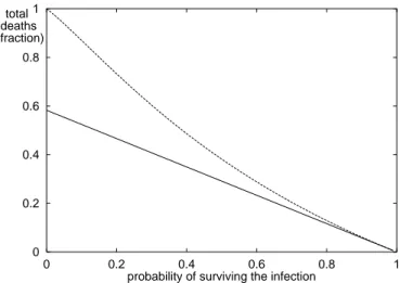
This optimization approach assigns payoffs (fitness) to each strategy without regard to the mix of strategies in the population, so there is a tacit as-sumption that each individual is “playing against nature.” If individuals “play against each other” so that payoffs depend on what others are doing, then evo-lution is not expected to maximize the population growth rater. An artificial but instructive example is a one-locus, two-allele haploid organism in which the fecundity of the wild-type allele A1isW1 =W0−p, and that of a mutant
A2 is W2 = W0− p2, where p is the frequency of the mutant in the
popu-lation. Then, once the mutant arises (p > 0), the mutant allele has higher reproductive success and increases in frequency up to p=1. This leaves the population with the minimum possible reproductive success. The optimization approach fails in this case because vital rates are frequency-dependent. Instead of seeking an optimal life history, we seek one that is an evolutionarily stable
strategy (ESS), meaning a strategy that is better than any other when the
en-tire population adopts that strategy. The optimality and ESS versions of life history-theory are now central to much of evolutionary and behavioral ecol-ogy, with an enormous literature. Fortunately, some good introductory surveys are available (Stearns 1992; Roff 1992; Bulmer 1995; Krebs and Davies 1987; Krebs and Davies 1993).
My goal here is to explain and illustrate how the optimality and ESS versions of life-history theory can be extended to deal with environmental “noise”: unpredictable fluctuations over time in environmental conditions, and hence in reproduction or survival rates. As modelers we often choose to ignore small random fluctuations, but temporal variation in vital rates can be enormous. In a review of published studies on variation in recruitment, Hairston, Jr. et al. (1996) found that reproductive success of long-lived adults varied from year to year by factors up to 333 in forest perennial plants, 4 in desert perennial plants, 591 in marine invertebrates, 706 in freshwater fish, 38 in terrestrial vertebrates, and 2200 in birds. These figures represent the variation among years when some reproduction occurred; many of the studies also report years in which reproduction failed completely. Similarly, the re-cruitment success of diapausing seeds or eggs varied by factors of up to 1150 in chalk grassland annual and biennial plants, 614 in chapparal perennials, 1150 in freshwater zooplankton, and 31,600 in insects. In such cases, a the-ory based on average conditions seems hard to justify. To introduce “noisy” life-history theory in a simple setting, I will first review the classical theory of emergence-from-dormancy strategies for seeds or eggs in temporally fluctuat-ing environments (Sections 1.2 and 1.3), emphasizfluctuat-ing methods over biology. This provides the necessary background for the main case study, the evolution of going-into-dormancy strategies in a freshwater copepod, Diaptomus
san-guineus. I asked the students in the course what they hoped to learn from my
1.2
HOW TO GAMBLE IF YOU’RE A SEED
Seeds of desert annual plants were one of the main motivations for Cohen’s (1966) model, sketched in Figure 1.1. At the start of growing season
Figure 1.1. Cohen’s (1966) model for optimal dormancy strategies in seeds of annual plants. At census times 0, 1, 2,. . . the population consists entirely of dormant seeds. The state variable for the model isn(t), the total number of dormant seeds at census timet. Seeds that remain in dormancy have a constant risk of death, while seeds that germinate face a random and unpredictable set of conditions affecting their chances of completing the adult life cycle and producing a crop of new seeds.
t, there aren(t)buried seeds (or eggs) that have the choice of “hatching” or not. The seeds that hatch each produceYtnew seeds that reenter the seed bank
and survive until the start of growing season(t+1). For simplicity I will follow Cohen’s original model and assume that theYt values in successive years are
independent and identically distributed (but really nothing is changed under the weaker assumption thatYt is stationary and ergodic). Of those that don’t
hatch, a fractionssurvive to time(t+1). Then ifHis the fraction that hatch, the population dynamics are
n(t+1)=[H Yt+(1−H)s]n(t). (1.1)
We assume for now that H is constant: seeds are not able to predictYt and
adjust their germination accordingly. Under what conditions is it then best for some seeds to “sit it out” until next year(H<1)?
This may seem like an odd way to specify an evolutionary model: where are the genes, Mendel’s laws, and the fitness differentials that drive evolution? But (1.1) has all the necessary information, if we adopt the simpli-fying assumption that “like begets like”: all offspring have the sameHas their “mother”. This can be given some respectability by calling it a haploid asexual model. Each genotype’s abundance then obeys (1.1) with its own value ofH, and the changes in abundance translate into changes in genotype frequencies. If we’re lucky, we can get away with this, and the outcome of selection will be the same under more reasonable assumptions about inheritance (see below).
Under “like begets like,” the winner is the type with the highest long-run growth rate, which we can calculate as follows. Denote λ(t) = [H Yt+(1−H)s], so that
n(t+1)=λ(t)n(t). (1.2)
divide byt. This gives us
1
t log(n(t))= 1
t log(n(0))+ 1 t
t−1 X
j=0
log(λ(j)). (1.3)
As t → ∞, the first term on the right-hand side in (1.3) goes to zero. The second term converges, by the strong law of large numbers (or the ergodic theorem, if you prefer), toElog(λ(t)), which is therefore the long-term growth rate analogous tor defined by the Euler-Lotka equation (above). Thus the winningHis the one that maximizes
ρdef=Elog(λ(t))=Elog [H Yt+(1−H)s]. (1.4)
One immediate consequence of (1.4) is that the per capita reproductive success Yt must be greater than 1 on average. Applying Jensen’s inequality to the
logarithmic function in (1.4), we have
ρ=E[log(λ(t))]<log[E(λ(t))]=log [H E[Yt]+(1−H)s]
(1.5)
so long as the variance of λ(t)is nonzero. So when E[Yt] ≤ 1, it follows
thatρ < log(1) = 0, a negative long-term “growth rate” implying that the population is (in the long run) decreasing to zero. Thus any viable population must haveE[Yt]>1, and from here on out I assume that to be true.
In addition, (1.4) can be used to qualitatively characterize and ap-proximate the winningH by curve-sketchingρ as a function of H. We can find the derivatives ofρ(H)by differentiating inside the expectation in (1.4) — the fastidious will observe that this does require some mild assumptions aboutYt — to get
ρ′(H) = E
Yt−s
H Yt+(1−H)s
(1.6)
ρ′′(H) = E
−(Yt−s)2
(H Yt+(1−H)s)2
<0 (1.7)
Because the second derivative is negative, there are only three possibilities (Figure 1.2). The optimum is at H = 0 if ρ′(0) < 0, i.e., if E(Y
t) < s;
this would mean that a seed should follow Peter Pan and avoid the trials of adulthood by refusing to grow up. The optimum population growth rate is then ρ(0)=log(s) <0, implying that the population decreases to zero abundance for any value of H. So for any real population this possibility is actually impossible. The optimum is atH =1 ifρ′(1)≥1, i.e., if 1−s E[1/Yt]≥0,
and otherwise at some 0< H <1. Thus we have found the condition under which some seeds should “sit it out” each year:
Optimal H<1 if s E
1 Yt
>1. (1.8)
Figure 1.2. Curve-sketching ρ(H) for Cohen’s (1966) model. Because ρ(0) =
log(s) <0 andρ′′(H) <0, there are only three possibilities, determined by the sign ofρ′at 0 and 1. Ifρ′(0) <0 , thenρ(H)is everywhere negative and the population cannot survive for any H (curve 1). Ifρ′(0) >0 andρ′(1) >0 (curve 2), thenρ is maximized at H =1. Only forρ′(0) >0 andρ′(1) <0 is the optimalHbetween 0 and 1 (curve 3).
small-variance case proceeds by writing random quantities as their mean plus random deviations, e.g.,Yt=Y¯+σ εt, whereE(εt)=0, Var(εt)=E(εt2)=1,
andσ2 is therefore the variance ofYt. We then pretend that the variance is
“small” and do a truncated Taylor expansion aboutσ =0:
E1Yt
= E
1 ¯ Y+σ εt
= 1¯ YE
1 1+(σ/Y¯)εt
(1.9)
= 1¯
Y E[1−(σ
¯
Y)εt+(σ
¯
Y)2ε2t − · · ·]∼= 1 ¯ Y[1+(σ
¯
Y)2].
Substituting into (1.8), the “small-fluctuations” condition for H < 1 to be optimal is that
(sY¯)1+(σ/Y¯)2>1. (1.10)
Because we are assuming ¯Y > 1 (as argued above), we haves/Y¯ <1. The interpretation of (1.10) is therefore that all seeds should hatch each year if the variance in reproductive success (σ2) is small, while if the variance is large some seeds should sit it out.
The good years/bad years case is to suppose thatYt = M ormwith
probabilities pand 1−prespectively, wherem≪1≪ M. Then from (1.6) we calculate directly
ρ′(H) = p
M −s H M+(1−H)s
+(1−p)
m−s H m+(1−H)s
∼
= Hp − 1−p
1−H (1.11)
1− p. Because ¯Y > 1 buts < 1, the expected number of seeds next year (new plus survivors) is always maximized atH =1. Thus a conclusion from both cases is that when environmental variation is high, organisms should
bet-hedge: reduce their average yield in order to have a hedge against occasional
misfortune. The same principle applies to many traits other than dormancy (Seger and Brockmann 1987; Phillipi and Seger 1989).
One unpleasant aspect of this analysis is that population density in-creases without limit, for many “losers” as well as the “winner” phenotype. This behavior results from the simplifying assumption that the per capita fe-cundity Y is unaffected by crowding. The simplest way of imposing limits to growth is to assume that per capita reproductive success is affected by the overall density of competitors, sayYt = KtF(Nt), where Kt is random and
Nt =
P
i Hini(t)is the total number of seeds emerging from dormancy (i
run-ning over all types in the population). The key simplifying assumption in this model is that the population is well mixed; i.e., it assumes that spatial varia-tion in the density of competitors is small enough to ignore. Because seeds are now pitted against each other, instead of an “optimal” strategy we seek a “win-ning” ESS: a typeH such that any other type is at a disadvantage when type H dominates the population. Formally, letY∗
t(H)denote the value ofYt in a
population consisting entirely of type-H individuals. Then the logic behind (1.2) and (1.4) still applies to give the growth rate of a rare typehinvading an otherwise all-Hpopulation:
ρ(h|H) = EloghYt∗(H)+(1−h)s (1.12) ∂ρ
∂h = E
Yt∗(H)−s hYt∗(H)+(1−h)s
(1.13)
(the formal derivation considers a mixed population with typehrare, and lin-earizes the dynamics of typeharoundh =0 (Chesson and Warner 1981; Ell-ner 1985; Chesson and EllEll-ner 1989)). As in (1.7) we then have∂2ρ∂h2<0, so for anyHthere is a single “best” invader, and an ESSH∗is defined by the
property of being the best invader of itself:
∂ρ
∂h =0 at h =H=H
∗. (1.14)
The conditions favoring dormancy can be found as in the density-independent model, by asking whether H = 1 can be invaded by h < 1 (i.e., whether ∂ρ/∂h <0 ath = H =1). The formal calculations are the same as before, and the result is (1.8) withYt replaced by theYt∗forH =1.
The analysis of (1.8) is more difficult in the density-dependent case, because Y∗
t is only defined implicitly through the nonlinear dynamics of a
single-type population. So before we can evaluate the expectation in the ESS criterion and thereby determine the success of the invader, we first have to find the long-term (stationary) distribution of the resident type. So it’s time for one more gambit: we will choose an especially convenient form of density dependence, F(N) = 1/N. This is convenient because it implies that the total number of new seeds in yeart is exactlyKt. Then when the population
consists of a single type with H = 1, we have Nt = Kt−1 — all seeds on
Y∗
t(H)=Kt/Nt =Kt/Kt−1. Substituting these into (1.8) and simplifying, the
condition for dormancy to be advantageous iss E[Kt]E[1
Kt]>1.
As in the density-independent case, one can get a good feel for what this formal condition says by looking at special cases. I leave that for you to do by yourself as an EXERCISE to see how well you have followed the story so far:
Derive and interpret the small-fluctuations and good years/bad years conditions for H∗ < 1. You should discover that the good
years/bad years result is now very different:H∗=1 if good years
are either very frequent or very infrequent. Why is this? — give an intuitive, nonmathematical explanation. Check your results by writing a program to simulate competition among multiple (10– 25) types with differentH-values; run it first at parameter values where H =1 should win, and then at parameters where H =1 should lose.
There’s a useful way of rewriting the ESS condition∂ρ/∂h =0. From (1.13) we see that the ESS condition is equivalent to
E
Y∗
t(H)
hY∗
t(H)+(1−h)s
=E
s
hY∗
t(H)+(1−h)s
(1.15)
and therefore each of the expectations must in fact equal 1 (because h × (right hand side)+(1−h)×(left hand side)=1). It’s hard to wring any deep biological meaning from this way of characterizing the ESS, but it often turns out to be the most useful form of the ESS condition for mathematical pur-poses. It was used by Sasaki and Ellner (1995) and Haccou and Iwasa (1995) to analyze models for ESS bet-hedging with a continuum of options, and Mc-Namara (1995) has used this characterization to derive numerical methods for obtaining ESS’s in a general class of models that cannot be solved analytically (McNamara et al. 1995).
1.3
PROCEED WITH CAUTION
We know that evolution involves
1. Dynamics governed by Mendelian genetics.
2. Competition among a suite of genotypes for different trait values.
To do an ESS analysis we pretend that it involves
1. “Like begets like”: uniparental reproduction, effectively clonal.
2. Pairwise competition between an “established” and a rare “invader” type.
then essential to figure out who’s the boss — which individuals’ genotypes determine the outcome — and to model the power structure correctly. Germi-nation can have this complication if competition is localized in space (Ellner 1986). (2) An ESS can’t be dislodged once it is established, but that doesn’t guarantee that evolution will move the population to the ESS, even under “like begets like” (Eshel and Motro 1981; Takada and Kigami 1991). A strategyx∗ with the latter property is called a CSS (continuously stable strategy). For a scalar strategy parameter, a CSS is defined by the property that ifxis nearx∗ andyis betweenxandx∗and near tox, thenycan invadex.
Therefore the essential last step in an ESS analysis is to check
our-selves. The available checks are general theory, special cases, and
simula-tion. “General theory” is a set of results giving conditions under which an ESS analysis agrees with the outcome of evolution in a proper genetic model (Charlesworth 1980; Taylor 1989). Almost all of these rely on weak-selection approximations, so they offer comfort but not certainty. Convenient special cases of the genetics can often be used to check the “like begets like” gambit by raising the likely complications in the simplest possible setting (e.g., few locus, few allele diploid with strong selection). Simulation is often the only way to check the pairwise competition gambit, because multitype competition models are high dimensional.
1.4
HOW TO GAMBLE IF YOU’RE A COPEPOD
A conflict between existing theory and experimental data usually means that there’s useful work to be done. This conflict walked into my office in the form of Nelson G. Hairston, Jr., explaining a mismatch between pop-ulation genetics theory and the diapause behavior of the copepod Diaptomus
sanguineus in Bullhead Pond, Rhode Island.
Hairston studied the switch-date of an adult female: the date each spring when she switches from laying clutches of immediate-hatching eggs (that hatch in a few days) to laying diapausing eggs that remain dormant at least until the next fall. Copepods don’t carry calendars, but they can use photoperiod and temperature to tell the time of year. Diapausing eggs are safe from predation by fish, which intensifies when the fish become more active as the pond warms up in spring. The increase in fish activity is rapid enough that as a first cut we can imagine all fish suddenly becoming active on a single
catastrophe date each year (Figure 1.3a).
(a)
(b)
(c)
Figure 1.3. Switch-date evolution in Diaptomus sanguineus. (a) Summary of the life cycle. From late spring through fall, the population consists entirely of diapausing eggs. In early winter, fish predation declines and eggs begin to hatch out, producing im-matures and then adults in the water column. Adults initially lay immediate-hatching (“subitaneous”) eggs and then switch to producing diapausing eggs. (b) Average fre-quency distribution of switch date for 1979–1989. (c) Switch date evolves in response to year-to-year fluctuations in predation intensity. Thex-axis is fish density relative to its mean and the y-axis is the between-year change in population mean switch date, scaled by the standard deviation of switch date in the initial year. The regression (solid line) is significant (from Hairston, Jr., and Dillon (1990)).
following a year of high fish density and shifts later after a year of low fish density (Figure 1.3c).
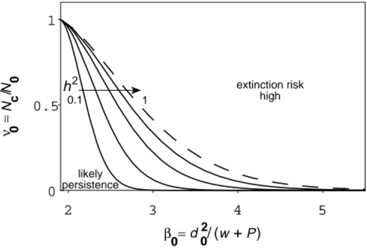
dates in different years, or else a bet-hedging strategy in which individu-als with a common genotype have different switch dates. Lab experiments showed that a large part of the variation is heritable (heritabilityh2 ∼0.5 for photoperiod response). The extant population genetics theory for fluctuating selection was interpreted as showing that temporally fluctuating selection on a quantitative trait only maintains genetic polymorphism under very special circumstances (primarily, if the fluctuations act to create heterozygote advan-tage) (Hedrick 1986; Bull 1987; Karlin 1988; Turelli 1988; Barton and Turelli 1989; Frank and Slatkin 1990; Gillespie 1991). So there were three (nonexclu-sive) possibilities: the variation was due to nonadaptive mutation; the theory was incorrect; or the theory was mathematically correct but had been misin-terpreted, and the conclusions were in fact not applicable to Diaptomus.
We suspected that the theory was correct but not applicable to
Diap-tomus. Like most population genetics theory it used the conventional
assump-tion of discrete nonoverlapping generaassump-tions, and the interpretaassump-tion of the re-sults tacitly ignored the possibility that overlapping generations could change the results. Diaptomus has overlapping generations due to eggs remaining in diapause for several years (Stasio 1989; Hairston, Jr. et al. 1995); the annual survival rate of diapausing eggs is over 98%, and eggs can remain viable in the sediment for up to 300 years (Hairston, Jr. et al. 1995), although eggs older than a decade or two probably have slim chances of hatching because they are too deeply buried in the sediment. In ecological models for interspecific competition, overlapping generations greatly increase the range of conditions under which environmental fluctuations can lead to coexistence (Chesson and Warner 1981; Chesson 1994; Shmida and Ellner 1984).
We therefore set out to show that the effect of generation overlap is similar in genetic models, beginning with a “cartoon” genetic model for switch date derived by modifying (1.1) as little as possible. We assumed that the com-peting types differ in switch date but all have the same hatching fraction (H). Relative values of reproductive successYt for each genotype were assumed
to be a functionw(d −θt), whered is a female’s switch date, θt is the
opti-mal switch date in yeart, andwis a selection function that penalizes wrong guesses, such as the Gaussianw(z)=exp(−z2/2v2). The essential properties ofw are that it is maximized when the female uses the best switch date for this year’s catastrophe date (d =θt)and decreases with worse guesses (larger
|d−θt|). It is convenient to shift the time scale so thatE(θt)=0. Absolute
reproductive success was defined in the model by assuming (for convenience) that the total egg production in each year is constant (K).
For ESS analysis of this model, as usual we consider a rare type (z= d) invading a common type (z = D). Let Nt denote the abundance of the
common type and nt the abundance of the invader — as in the seed-bank
model, these are the numbers of diapausing eggs just before hatching time in yeart. In competition with the invader, the common type’s share of the total egg productionK is
K H Ntw(D−θt)
H ntw(d−θt)+H Ntw(D−θt)
. (1.16)
Because the invading type’s abundance is taken to be negligible, this reduces to simply K. Therefore Nt+1 = K +s(1−H)Nt, and in the long run Nt
now compute the growth rateρ for the invader. The invading type’s share of the total egg production is
K ntw(d−θt)
ntw(d−θt)+Ntw(D−θt)
(1.17)
so the per capita egg production by invading-type eggs is
Kw(d−θt)
H ntw(d−θt)+H Ntw(D−θt)
. (1.18)
In the denominator nt is again negligibly small compared to Nt, and Nt =
K/(1−γ ), so the per capita egg production of the invader reduces to
Yt=
(1−γ )w(d−θt)
Hw(D−θt)
. (1.19)
Thus the growth rate for the invader is
ρ(d|D) = Elog[s(1−H)+H Yt]
= Elog
γ +(1−γ )w(d−θt) w(D−θt)
. (1.20)
where the expectation is over the distribution of the random environmentθt.
Note thatρ(x|x)=0 for allx, as it should be.
These minor changes to the optimal diapause models turned out to have the consequence we were hoping for: coexistence of multiple switch dates when Var(θt) is large, rather than a single ESS switch date (Ellner and
Hairston, Jr. 1994). To hold the algebra down I will consider the Gaussian selection function, choosing time units so thatv2 = 1 and thereforew(z) = exp(−z2/2); essentially the same qualitative behavior holds for any smooth
symmetric selection function. As usual we can characterize the ESS via the derivatives ofρ: to be an ESS, a trait value D∗must satisfy∂ρ∂d =0 and ∂2ρ∂d2<0 atd =D=D∗.
For this model we get
∂ρ ∂d =E
(1−γ )w′(d−θ )/w(D−θ ) γ+(1−γ )w(d−θ )/w(D−θ )
, (1.21)
which atd =D=D∗ simplifies to ∂ρ
∂d = −(1−γ )D
∗. (1.22)
Thus the only possible ESS is D∗ =0, the optimal switch date under average conditions (recall that E(θt) = 0). Differentiating within the expectation in
(1.21) and evaluating for Gaussianwatd=D=D∗gives
∂2ρ ∂d2(D
∗,D∗)=(1−γ )σ2
θγ−1
(1.23)
whereσ2
d = D = D∗ in this case, which implies that ρ(D∗|d) > 0 ford near D∗.
Becauseρ(D∗|d) >0 is the growth rate for the ESS invading a non-ESS type, we can conclude that the ESS can always invade nearby types. On the other hand, whenσθ2γ >1, (1.23) is positive, soD∗ is not an ESS.
Trait value x
rho
-0.4 -0.2 0.0 0.2 0.4
-0.05
0.05
0.15
Sigma=1.0, D*=0 is an ESS
x invading D*=0 D*=0 invading x
Trait value x
rho
-0.4 -0.2 0.0 0.2 0.4
0.0
0.1
0.2
0.3
0.4
Sigma=2.0, D*=0 is not an ESS
x invading D*=0 D*=0 invading x
Figure 1.4. Shape of the boundary growth ratesρ(x|0)forx invading D∗ = 0, and
ρ(0|x)forD∗=0 invadingx. The top panel shows the situation below the threshold for maintaining genetic variance. D∗is an ESS because it cannot be invaded by nearby types (ρ(x|0) <0). In our modelD∗can also invade nearby types (ρ(0|x) >0), though in general an ESS need not have this property. Above the threshold (bottom panel)D∗ is no longer an ESS because it can be invaded by nearby types, but it retains the ability to invade nearby types (ρ(0|x)andρ(x|0)are both positive).
The corresponding picture is in Figure 1.4. Forσ2γ < 1, D∗ = 0
resists invasion by nearby types (i.e.,ρ(x|D∗) <0) so it is an ESS; moreover it can itself invade nearby types (i.e.,ρ(D∗|x) >0). Forσ2γ >1, D∗ is still
able to invade nearby types, but it is vulnerable to a reinvasion by those same types (ρ(x|D∗) >0) so it is not an ESS. Consequently there aren’t any
possi-ble types that cannot be invaded by some other nearby type, so we expect that genetic variability will be maintained indefinitely. Simulations of multigeno-type competition with a wide range of parameter values matched the results of this ESS analysis (Ellner and Hairston, Jr. 1994).
as usual leads to
ρ(z|−x,x)
(1.24)
= Elog
γ+(1−γ ) w(z−θt)
ptw(x−θt)+(1−pt)w(−x−θt)
where ptis the frequency of typexin yeart, and the expectation is with respect
to the joint distribution of(θt,pt), which is a mess. It’s a bit simpler to assume
that the values ofθtin different years are independent, implying thatθtandpt
are independent, but we still need the distribution of ptto evaluate (1.25). We
failed to find a general solution, and resorted to treatingδ=(1−γ )as a small parameter to allow small-fluctuations approximations to the dynamics of pt
and to the integrand in (1.25). Forσ2
θ just above the threshold the necessary derivatives can be gotten from Taylor expanding in x andz(which are near 0). Far past the threshold a different approximation is needed. If x is very large, then in most years one of the pair{x,−x}will fare much better than the other, and it is a good approximation to pretend that the other has no offspring at all. I’ll spare you the technical details — in fact we spared ourselves the details, doing most calculations by programming them in MAPLE — but in the end it works, giving approximations that allowed us to derive the first few bifurcations in the ESS whenσθ2exceeds the threshold (Figure 1.5).
Figure 1.5. The first bifurcation in the ESS trait distribution as the selection variance increases past the threshold for maintaining genetic variance. These plots compare simulation results on competition among a large set of competing types (solid squares) with the asymptotic approximations that are the basis for studying subsequent bifurca-tions. Solid line: approximation for near the threshold. Dashed line: approximation for far above the threshold. See the text and Ellner and Sasaki (1996) for further details.
Above the threshold valueσ2
crit, the “like-begets-like” gambit fails
at the first locus with(0,0),(z,0),(z,z)at the second (0 denotes the unmu-tated wild-type allele at the second locus). These kinds of complications mean that the precise form of variation is sensitive to hard-to-estimate quantities, and to questionable simplifying assumptions (symmetric selection, additive gene effects, etc.).
However, all the results for specific models that we examined have the same qualitative pattern: the variation consists of a few alleles of large effect at each locus affecting the trait (Ellner and Sasaki 1996; Ellner 1996). Another general result (Sasaki and Ellner 1996) is that the covariance components of the genetic variance (i.e., the correlations between loci affecting the trait, and between maternal and paternal contributions at each locus) are all positive for all polymorphic loci determining the trait.
These qualitative predictions are important because they allow exper-imental tests of the fluctuating-selection hypothesis. For example, covariance components can be estimated by conceptually simple laboratory breeding ex-periments. Under random mating in the absence of selection, the changes in trait variance from generation to generation are a function of the underlying covariance components (Falconer 1981). This makes it possible to estimate the genetic covariance components simply by estimating the distribution of trait values in the population for several successive generations. These esti-mates need not be terribly precise, because it is their sign rather than their numerical value that distinguishes between the fluctuating-selection hypothe-sis and the alternative of mutation-selection balance.
1.5
OLD AND IN THE WAY
But before rushing out to test the predictions from a deliberately sim-plified model, it’s a good idea to check that they aren’t artifacts of the simpli-fying assumptions. We therefore examined models with nonheritable variation (Sasaki and Ellner 1995), models with density-dependent fecundity and fluc-tuating population size instead of “constantK” (Ellner and Sasaki 1996; Babai and Ellner, in prep), and models with age or stage structure (Ellner 1996).
In this section I will briefly consider models with population struc-ture, because they involve some important new concepts and techniques, and because the assumption that “an egg is an egg is an egg” — whether one year old or twenty — is probably the most egregious error in the cartoon copepod and seed-bank models. Older eggs or seeds may deteriorate or become too deeply buried to encounter the conditions required for successful emergence from dormancy.
As a first step, consider a deep-shallow model (Easterling 1995) in which any eggs that don’t hatch the year after they were produced become covered by sediment and can only hatch if some disturbance mixes them back up to the top (Figure 1.6). These older eggs then have a far lower hatching rate than newly produced eggs. Equation (1.1) for a single typexis replaced by:
n0(x,t+1) = [H0n0(x,t)+H1n1(x,t)]Yt (1.25)
n1(x,t+1) = (1−H0)sn0(x,t)+(1−H1)sn1(x,t)
wheren0(x,t)is the number of newly produced type-x eggs (age< 1 year)
Figure 1.6. The deep-shallow egg-bank model motivated by Diaptomus sanguineus. This model distinguishes between newly produced “shallow” eggs, and older “deep” eggs that have become covered by a layer of sediment at the pond bottom.
capita yield for typexis
Yt=
Kw(x−θt)
P
y[H0n0(y,t)+H1n1(y,t)]w(y−θt)
. (1.26)
For an ESS analysis we consider as usual an infinitesimally rare invader d competing with established type D; the per capita yield for the invader (1.26) then becomes
Yt =
Kw(d−θt)
[H0n¯0+H1n¯1]w(D−θt)
(1.27)
where ¯ni is the equilibrium value of ni(D,t) in the absence of competitors
( ¯n0 = K,n¯1 = (1−H0)s K/(1−(1−H1)s)). With (1.27) substituted into
(1.26) the equation for the invader is linear (as always) and can be written in matrix notation as
n0(d,t+1)
n1(d,t+1)
=
H0Yt H1Yt
(1−H0)s (1−H1)s
n0(d,t)
n1(d,t) .
(1.28)
The good news about (1.28) is that the invader’s growth rateρ(d|D) still exists, and is a nonrandom quantity under fairly mild technical conditions; the bad news is that there is no longer a general closed formula forρ analo-gous to (1.4) (Furstenberg and Kesten 1960; Tuljapurkar 1990). Only in very special cases is there an explicit formula forρ; for example, if all eggs hatch either in their first year or in their second (Tuljapurkar and Istock 1993).
The only practical way available for getting around this problem is to use the small-fluctuations approximation toρ(d|D). This approximation is derived by writing A(t)= A¯+εB(t)where ¯A=E[A(t)], followed by a long string of clever calculations to get the first two terms in a Taylor expansion for ρaboutǫ=0 (Tuljapurkar 1990; Derrida et al. 1987). If the matricesA(t)are independent and identically distributed (as in the models here), the result is:
ρ=logλ1−
ε2 2λ21
X
i,j,k,l
whereλ1is the dominant eigenvalue of ¯A,
⇀
vw⇀, are the corresponding left and right eigenvectors normalized tohw,⇀ ⇀vi =1 and Cov(i j,kl)is the covariance betweenBi j(t)andBkl(t). If the matrices A(t)are not independent, then there
are additional terms resulting from covariances between Bi j(t) and Bkl(t −
m),m=1,2,3, . . .. Tuljapurkar (1990) presents a general derivation; Derrida et al. (1987) use a different approach that leads to a simpler derivation for independent matrices.
The most important thing to realize about (1.29) is that it’s not nearly as bad as it looks. After a few practice problems to get yourself oriented it really is a usable tool. Moreover, for many ESS analyses, (1.29) can actually be used to derive exact (rather than approximate) local stability results, by getting the leading terms in a Taylor expansion ofρ(D+ε|D)inε, and infer-ring from those the partials ofρthat figure in the ESS analysis. Ellner (1996) uses this approach to carry out the ESS analysis for a more general model of a population with age, stage, or spatial structure.
The conclusion (Ellner 1996) is that structure doesn’t matter very much at all for the maintenance of genetic variance. As in the unstructured model, the threshold for maintaining genetic variance is σθ2γ > 1 for the deep-shallow model, and also for models with far more general age or stage structure. The only difference is that the generation overlapγ must be com-puted in units of Fisher’s reproductive value (Appendix A) — i.e., instead of counting all eggs equally, weight them by their reproductive value and letγ be the fraction of the current total that survives to next year. Reproductive values show up because they are given by the dominant left eigenvector of A0 (Caswell 1989), which appears in both the small-fluctuations
approxima-tion and the eigenvalue sensitivity formula. That’s another reason why (1.29) isn’t so bad: you can probably give a meaningful interpretation of the results even if you can’t calculate⇀
v, ⇀
worλ1 explicitly, because you know what they
represent about the population.
1.6
THEORY MEETS DATA
Back to the copepods: does the theory actually apply to Diaptomus in Bullhead Pond? We have made two checks of the fluctuating-selection hypothesis against the available data.
fe-male’s hatching date, her switch date, and the catastrophe date (onset date of fish predation). The computation of R0 is based on a stage-structured matrix
population model, with parameters estimated directly from field or lab studies: stage durations from bottle experiments in the field; survivorships of preadult stages from population sample data; reproductive schedule from field data on clutch size and lab observations of the interclutch interval. The onset date and intensity of predation each year were taken from Hairston, Jr. (1988), adding subsequent years’ data. The averageR0for each switch date (averaged
over the observed distribution of hatching dates) is then the measure of fitness. This was applied to each year’s switch-date distribution to predict the total di-apausing egg production, the per capita didi-apausing egg production, and the mean switch date in the following year.
The results for egg production are quite good (Figure 1.7). The model
a b
Figure 1.7. Predictions of the a priori selection model compared with estimates of egg production within a year, and year-to-year changes in mean switch date. The solid line in each panel is observed = predicted. The dashed line in panel (b) is the unconstrained linear regression of observed on predicted, omitting the “outlier” (circled).
also predicts the trend in year-to-year changes in switch date, but there is considerably more scatter. This can partially be explained by a factor omitted from the model: eggs hatching out from deep in the sediment which did not experience the most recent round of selection. Indeed, the extreme high outlier was from a year when pond drying resulted in an exceptionally high hatch-out of more deeply buried eggs.
Our second check was a laboratory test of the prediction that the egg bank acts as a “reservoir” of genetic variance in switch date. Eggs were col-lected from the sediment and the water column, and the distribution of switch date was determined in the lab for each of these subpopulations (after several generations of within-subpopulation random mating in the lab, to eliminate effects of the environment experienced by the founding eggs). The prediction was that switch-date variance should be higher in the sediment-derived sub-population. Instead, there were no detectable differences in variance of switch date, but rather large differences in the mean switch date (Hairston, Jr. et al. 1997).
sense in terms of the theory developed in Sections 1.2 and 1.4 of this chapter. Genotypes with an early switch date never encounter fish predation, so these genotypes perceive a relatively constant environment and should have a high value of H. Similarly, late-switching genotypes perceive a highly variable environment and should have a low value of H. This correlation is what we appear to see in the experimental data (Hairston, Jr. et al. 1997). Eggs with a higher propensity to hatch (either earlier hatching in the lab, or being found in the water column rather than the egg bank) also had an earlier mean switch date in the lab. These observations do not show unequivocally that the correla-tions are due to genetic differences rather than maternal effects or other forms of nonheritable variation. Regardless of the mechanism, our basic assumption that all switch-date genotypes have the sameH turned out to be incorrect.
With this added layer of complexity, quantitative predictions of the model become even more sensitive to the fine details. If you choose every-thing just right, allowing Hand switch date to coevolve can generate the ob-served correlations (Figure 1.8); but change things a bit (high recombination rate, constantK,. . . ) and the correlations can be reduced to nil or reversed. So for now we can only say that the fluctuating-selection hypothesis is consis-tent with all available experimental data and generates good predictions of the short-term responses to selection.
1.7
CODA
Even if you don’t care especially about copepods or genetic variance, this case study illustrates some benefits of combining theoretical and experi-mental approaches in biology. The most important benefit is the opportunity for creative tension when theory and experiments don’t line up as perfectly as hoped. This can be simply a matter of theoreticians using preexisting experi-mental data, or experiexperi-mental ecologists browsing the latest issues of theoreti-cal journals for inspiration. But much of the “added value” accrues from real feedback between theory and experiments, theory provoking experiments that in turn force changes in the theoretical models, generating new predictions and calling for further experiments. Although we still cannot present compelling evidence that our (improved) theories are a complete and correct explanation for our (more extensive) data on Diaptomus, the new theory and the new data are both valuable in themselves.
Switch date D
Hatching fraction H
-4 -2 0 2 4
0.0 0.2 0.4 0.6 0.8 Sigma=1.0
Switch date D
Hatching fraction H
-4 -2 0 2 4
0.0 0.2 0.4 0.6 0.8 Sigma=1.2
Switch date D
Hatching fraction H
-4 -2 0 2 4
0.0 0.2 0.4 0.6 0.8 Sigma=1.4
Switch date D
Hatching fraction H
-4 -2 0 2 4
0.0 0.2 0.4 0.6 0.8 Sigma=1.6
Switch date D
Hatching fraction H
-4 -2 0 2 4
0.0 0.1 0.2 0.3 0.4 Sigma=1.8
Switch date D
Hatching fraction H
-4 -2 0 2 4
0.0 0.1 0.2 0.3 0.4 Sigma=2.0
Switch date D
Hatching fraction H
-4 -2 0 2 4
0.0 0.1 0.2 0.3 0.4 Sigma=2.2
Switch date D
Hatching fraction H
-4 -2 0 2 4
0.0 0.1 0.2 0.3 0.4 Sigma=2.4
Figure 1.8. Simulation results for a haploid model with heritable variation in both hatch fraction (H) and the switch date (D). Each of the traits was assumed to be controlled by a single locus. The squares show how the long-term average genotype frequencies change as the selection variance increases. Initially there is a single type, with H decreasing as the variance increases. The initial bifurcation is to two values each for the Hand Dgenotypes, with a negative correlation betweenH andD. The model is essentially the same as the basic model in Section 1.4, except that the total diapausing egg production (K) is assumed to be higher in years when the optimal switch date is later (because the predation rate is lower in those years). This assumption is essential for generating the negative correlation betweenHandD.
should be discrete applies to any system with temporal or spatially fluctuat-ing selection (Sasaki and Ellner 1996); molecular genetic evidence consistent with this prediction has already been found in a number of terrestrial plant and animal species (Mitchell-Olds 1995).
This chapter has focused on a single case study, but the literature holds a lot of required reading for anybody intending to work on life history evolution in fluctuating environments. Here are a few starting points that will point you toward the rest of what’s out there. For models with heritable vari-ation, Charlesworth (1980) is a self-contained compendium of the rigorous (and as-rigorous-as-possible) theory for discrete and overlapping generations, though it is mostly about constant selection. Gillespie’s (1991) book similarly summarizes the theory for random selection with discrete, nonoverlapping generations. The overwhelming majority of the literature is about bet-hedging strategies where the variation is nonheritable, as in Section 1.2 of this paper. The reviews by Seger and Brockmann (1987) and Phillipi and Seger (1989) are excellent background, and the book edited by Yoshimura and Clark (1993) is a good introduction to the scope of recent work. Recently, McNamara (1995; 1996) has written a series of papers that unify and extend many prior results on optimal bet-hedging strategies. McNamara also uses his results to derive dynamic programming methods to calculate optimal strategies in models too complex for analytic solution, and I expect that these methods will inspire a burst of applications in the next few years.
ACKNOWLEDGMENTS I am grateful to all the organizers of the special year course, with special thanks to Fred for serving as the hospitality com-mittee; to the students for keeping me on track; and to Paul, Eric, and Pej for getting me camping in the Uintas by somehow neglecting to mention the snow. Eric Charnov and Jon Seger attended the lectures and kept me on my toes, and several of their comments and questions have been incorporated into the chapter.
REFERENCES
Barton, N. H. and Turelli, M. 1989. Evolutionary quantitative genetics: How little do we know? Annual Review of Genetics, 23, 337–370. {12, 22}
Bull, J. J. 1987. Evolution of phenotypic variance. Evolution, 41, 313–315. {12, 22} Bulmer, Michael. 1995. Theoretical Evolutionary Ecology. Sunderland, MA: Sinauer
Associates, Inc. ISBN 0-87893-078-7 (paper), 0-87893-079-5 (cloth). Pages xi + 352.{4, 22}
Caswell, Hal. 1989. Matrix Population Models: Construction, Analysis, and
Interpre-tation. Sunderland, MA: Sinauer Associates, Inc. ISBN 0-87893-094-9
(hard-cover), 0-87893-093-0 (paperback). Pages xiv + 328.{3, 18, 22, 357, 360} Charlesworth, Brian. 1980. Evolution in Age-Structured Populations. Cambridge, UK:
Cambridge University Press. ISBN 0-521-29786-9 (paperback), 0-521-23045-4. Pages xiii + 300.{3, 10, 22, 357, 360}
Charnov, Eric L. 1993. Life History Invariants: Some Explorations of Symmetry in
Evolutionary Ecology. Oxford: Oxford University Press. ISBN 0-19-854072-8
(hardback), 0-19-854071-X (paperback). Pages xv + 167.{4, 22}
Chesson, P. L. 1994. Multispecies competition in varying environments. Theoretical
Population Biology, 45, 227–276. {12, 22}
Chesson, P. L. and Ellner, S. 1989. Invasibility and stochastic boundedness in mono-tonic competition models. Journal of Mathematical Biology, 27, 117–138. {8, 22}
Chesson, P. L. and Warner, R. R. 1981. Environmental variability promotes coexistence in lottery competitive systems. American Naturalist, 117, 923–943. {8, 12, 22} Cohen, D. 1966. Optimizing reproduction in a randomly varying environment. Journal