fertility schedules from abridged data
*Carl P. Schmertmann**
I develop and explain a new method for interpolating detailed fertility schedules from age-group data. The method allows estimation of fertility rates over any ine grid of ages, from either standard or non-standard age groups. The new method, called the calibrated spline (CS) estimator, expands an abridged fertility schedule by inding the smooth curve that minimizes a squared error penalty. The penalty is based both on it to the available age-group data, and on similarity to patterns of 1fx schedules observed in the Human Fertility Database (HFD) and
in the US Census International Database (IDB). I compare the CS estimator to a very good alternative method that requires more computation: Beers interpolation. The results show that CS replicates known 1fx schedules from 5fx data better, and its interpolated schedules
are also smoother. The conclusion is that the CS method is an easily computed, flexible, and accurate method for interpolating detailed fertility schedules from age-group data. Users can calculate detailed schedules directly from the input data, using only elementary arithmetic.
Keywords: Fertility. Interpolation. Splines. Penalized least squares.
Introduction
Demographers like precise data for exact ages, but unfortunately we oten get the opposite – noisy sample estimates aggregated into wide age groups. Worse, sometimes the age groups do not cover the entire range of interest for the behavior under study. With abridged, partial, or noisy data, demographic calculations oten require interpolation and extrapolation of age-speciic rates.
In this paper I introduce a method for itting detailed fertility schedules to coarse, possibly noisy data. The method exploits a large new dataset, the Human Fertility Database (HFD), to identify empirical regularities in fertility schedules by single years of age 12-54. It then uses these regularities in a penalized least squares framework to produce simple rules for expanding grouped data (usually 5fx estimates) into detailed rates over an arbitrarily ine
grid of ages that may extend outside the range of the original data (for example, below age 15 or above age 50).
The new method uses spline functions as building blocks, and identiies smooth fertility schedules that match group-level data closely while also conforming to patterns observed in the HFD. I call the result of the procedure a calibrated spline (CS) schedule. Its derivation uses some rather dense matrix algebra, but the end result is exceedingly simple: basic arithmetic with the grouped data and a set of predetermined constants.
Notation and derivation of the calibrated spline estimator
In the next two sections I explain and derive the CS estimator. Readers uninterested in the mathematical details may, without diiculty, skip ahead to the penultimate paragraph of the next section, beginning with The key point is….
Suppose that the fertility schedule can be well approximated by a weighted sum of K continuous basis functions:
θ θ 1 1 1 ) ( ) ( ) ( Kx xK K k k
kb a b a
a = = (1)
∑
≈over the reproductive age range [α,β]. In many applications demographers use a ine grid of ages {a1…aN} and assume that fertility is constant at some level fi within each small interval
) ,
[ 21
2
1Δ + Δ
− i
i a
a . In such applications the discrete version of φ is an Nx1 vector:
θ θ = B
⎥ ⎥ ⎥ ⎦ ⎤ ⎢ ⎢ ⎢ ⎣ ⎡ ʹ ʹ = ⎥ ⎥ ⎥ ⎦ ⎤ ⎢ ⎢ ⎢ ⎣ ⎡ = N N b b f f
f ⋮ ⋮
1 1
(2)
where bi΄is a 1xK vector containing the value of each basis function at a=ai, and B is thus an NxK matrix of known constants.
at 12.25, 12.75,…54.75. I use quadratic B-spline basis functions (BOOR, 1978; EILERS; MARX, 1996) over uniform knots at two-year intervals.1
When fertility data is reported as averages for age groups (call the groups A1…Ag), we need multipliers for aggregating f. The Nx1 vector f is related to the gx1 vector of group averages (called y from here on) by:
θ B G G = = ⎥ ⎥ ⎥ ⎦ ⎤ ⎢ ⎢ ⎢ ⎣ ⎡ = f f f y g ⋮ 1 (3)
where G is gxN with
∑
∈ ∈ = k i k i j ij A a I A a I G ] [ ] [and I[.] is a 0/1 indicator function. The ine grid f is
similarly related to single-year rates by:
(4) θ β α B S S = = ⎥ ⎥ ⎥ ⎦ ⎤ ⎢ ⎢ ⎢ ⎣ ⎡ − f f f 1 1 1 ⋮
where Sij=Δ⋅I[(
α
+i)−1 ≤ aj < (α
+i)].Objective and estimation strategy
Suppose that we observe y, a g x 1 vector of sample estimates for age group averages. We want to estimate the K spline weights θ (and ultimately, the N elements of the discretized schedule f) from the g estimates in y. When K>g (i.e., when there are more than g basis functions) itting and estimation requires additional identifying information of some kind.
I propose two criteria for a good schedule f: it should (1) closely it the observed data y, (2) have an age pattern similar to known single-year schedules – speciically, to schedules downloaded from the Human Fertility Database (HFD, 2012) and in the US Census International Database (SCHMERTMANN, 2003, ile III). For these criteria, which I call it and shape respectively, one can construct vectors of residuals that should be near zero for good schedules. These vectors are:
θ ε θ ε MSB S M GB G = = − = − = f y f y s f : Shape : Fit (5)
The M matrix for shape residuals has a complicated construction, but a simple interpretation. Construction is as follows. I irst assemble a 43x530 matrix F, comprising 304 single-year ASFR schedules from the HFD over ages 12…54,2 plus an additional 226
1 Speciically, basis functions come from the bs( ) function in R (R CORE DEVELOPMENT TEAM, 2011), with arguments x=seq(12.25, 54.75, .50), knots=seq(12,54,2), and degree=2. I retain the third through twenty-irst columns of the resulting matrix as an 86x19matrix B.
estimated single-year schedules from the US Census International Database (IDB) using the quadratic spline model and coeicients from Schmertmann (2003,ile III).3 Singular value decomposition F=UDV’ yields orthonormal principal component vectors in U’s columns. The irst three of these columns (call this 43x3 matrix X) account for approximately 95% of the variation in F, in the sense that projections of any single-year schedule s onto the column space of X have small errors:
(
)
s ss
e= − = I43−P
⌢ (6)
where P= X(X’X)-1X’ is the projection matrix for the column space of X.
Deining M=(I43-P), shape residuals in Equation (5) represent the portion of a single-year
schedule that is unexplained by linear combinations of principal components. In other words, shape residuals εs in Equation (5) are large for single-year schedules that have age patterns unlike those observed in the HFD and IDB.4
Each criterion can be converted into a scalar index of a schedule’s “badness” by calculating an appropriately weighted sum of squares. These scalar penalty terms have generic form:
} , {
1
s f c Pc = ε Vcʹ c− εc ∈
(7)
where Vc = E[εcεc’] is the covariance of εc.
The covariance matrix of itting errors εf can be approximated logically. Supposing that the
estimates in the vector y represent ratios of births to an average of W women sampled in each age group, and that a typical age-speciic rate is approximately 0.10, then with independent sampling errors across groups the covariance of εf is:5
( )
W g ff
f E I
V 10
1 )
( ʹ ≈
= ε ε (8)
and its inverse is:
(
)
gf W W I
V 1( ) 10
≈
−
(9)
These assumptions are crude, but results are not very sensitive to them. The main point is that with large sample sizes, schedules that it age group averages poorly get extremely heavy penalties.
For the covariance of shape residuals, we refer to the single-year schedules in the HFD. For each of the 1480 schedules (s) in the HFD single-year data, one can calculate es=Ms.
The average outer product of these HFD shape residuals serves as a covariance estimate:
) ( s s
s = e eʹ
V (10)
3 It is slightly clumsy to split the ive-year IDB schedules into approximate single-year schedules in order to include them in the analysis, but adding these schedules is important. The HFD does not yet include countries from Africa and Asia that have very distinct age patterns – in particular African schedules oten have relatively high fertility at ages 35+, and some East Asian schedules have extremely low fertility at ages below 25. Estimation of SVD principal components from a matrix that includes the wider variety of patterns in the IDB produces a much more representative set of “typical” age schedules. 4 More precisely, a schedule f has large shape residuals when S
f lies far from the column space of X. It is possible for f to have low shape residuals even if it is unlike any observed schedule, if f is well approximated by a combination of principal components that has no counterpart in the database.
Vs provides information about which ages are likely to have large or small residuals, and
about the age patterns among those residuals.6
Summing the penalties produces a single index that is appropriately calibrated to the available information about errors:7
(
)
(
W)
y y y y y W P P P W W s s s s f f f s f ʹ + ʹ − ʹ = ʹ + − ʹ − = ʹ + ʹ = + = − − − 10 2 ) ( ) ( ) ( ) ( 10 ) ( 1 1 1 R Q MSB V MSB GB GB V V θ θ θ θ θ θ θ ε ε ε ε θ (11) where(
)
B’G’GB B’S’M’V MSBQ 1
10 −
+
= s
W W (12)
and
(
)
BGRW = 10W ʹ ʹ (13)
Because QW is positive deinite, expression in Equation (11) has a unique minimum when
weights are θ*=QW−1RW y
. Thus, for estimated fertility rates y that come from samples of approximately W women per age group, the combination of basis function that minimizes the joint criterion in Equation (11) is a vector that I call the calibrated spline (CS) it:
y y
f =B = B QWRW = KW
−1 *
* θ (14)
The key point is that this complex derivation leads to a simple result: the optimal schedule f is a linear function of the observed data y. Given a sample size, the N x g matrix KW contains predetermined constants, so that we can write the CS vector f* as a weighted sum of g columns:
g g W
W y y
f = + +
⋮ ⋮ ⋯ ⋮ ⋮ ) column ( 1 ) 1 column (
* K K (15)
In principle, this framework allows a demographer to create customized, simple arithmetical rules for transforming fertility estimates from any set of g age groups into a schedule over an arbitrarily ine grid of N rates over any age span of interest. The method is particularly straightforward because the “parameters” for the empirical model are the estimated age-group fertility rates themselves, so that itting the model requires only multiplication and addition.
In practice, researchers can simplify further by using one of the pre-calculated KW
matrices, for W = 100, 1000, 10000, or 100000 and common age groups, available online at <http://calibrated-spline.schmert.net/REBEP>. For larger sample sizes, multipliers vary little from the W=100,000 case; I recommend using the W=100,000 constants for samples with W > 100,000. If the sample size is unknown, I recommend using W=1000. Ater selecting the right order of magnitude W for sample sizes a demographer can produce a schedule
6 Adding a small constant to each diagonal element of V
s before inverting stabilizes results considerably. I add 0.1 times the median value of the diagonal elements from Equation (10).
for ages 12.25, … 54.75 directly from age group averages y by multiplying f* = KW y as in
Equation (15).
Example its with HFD, IDB, and Brazilian data
The CS method outlined above works for any set of age groups, but I deal with two speciic examples in the rest of this paper – cases in which (a) data are available for g=7 age groups 15-19 through 45-49, as in the US Census International Database (IDB) and many other datasets, or (b) data are available for g=9 ive-year age groups 10-14 through 50-54, as in the HFD.8
GRAPH 1
Empirical basis functions for a itted schedule at half-year intervals over [12,55]
10 20 30 40 50
0.0
0.5
1.0
Age
15 20
25 30
35 40
45
10 20 30 40 50
0.0
0.5
1.0
Age
10 15
20 25
30
35 40
45 50
Source: Author’s calculations based on Equation (14).
Note: Each line represents one column of K10000. These curves are multiplied by 5fx values (g=7 and g=9 of them in top and bottom panels, respectively) and then summed to produce the inal CS it.
Graph 1 illustrates K10000 for the g=7 and g=9 cases, by plotting each column as a function
of age. For example, a unit increase in estimated 5f15 changes f* values at various ages by the
height of the line labeled “15”. A unit increase in estimated 5f20 changes f* according to the
line labeled “20”, and so on. Note that the range of estimated fertility f* may extend beyond that spanned by the input data: in the g=7 case the procedure produces estimated ASFRs below age 15 and above age 50, based on known regularities in the age pattern of rates.
Using Equation (14) or (15), basis functions in Graph 1 are multiplied by the observed y values and then summed to produce complete CS schedules over [α,β]. The top panel of Graph 2 illustrates the expansion of a set of g=7 ive-year estimates into half-year intervals, using IDB data from Uruguay. The input data for Uruguay, based on national data, are:
yURU = 10-3 x (49 116 135 99 54 16 2)’
United Nations data (UNSD, 2014) indicate that in 2002 there were approximately W=100,000 Uruguayan women in each ive-year age group, so K100000 based on g=7 is the
appropriate matrix to use.
Multiplying the y values by the columns of K and summing, as in Equation (15), produces an 86x1 vector f*=Ky for rates at half-year intervals over 12-55, shown in the top panel.
GRAPH 2
Calibrated spline (CS) schedules for Uruguay 2002 (g=7, top panel) and Austria 1952 (g=9, bottom panel), estimated at half-year intervals over [12,55]
Age
Uruguay 2002 (CS fit from g=7 five−year rates)
10 20 30 40 50
05
0
100
150
Age
Austria 1952 (CS fit from g=9 five−year rates)
10 20 30 40 50
05
01
00
150
Source: Schmertmann (2003: Supplemental, ile III) for Uruguay; HFD (2012) for Austria.
The age-group averages for the CS model do not exactly replicate the input data. For example, the average of the CS schedule over ages 35-39 in Uruguay is .0536, slightly lower than the original 5f35 value of .0540. This occurs because minimizing the penalty index in
Equation (11) requires tradeofs between model it and the shape of schedule. The tradeof for Uruguay was typical, in the sense that over all 226 IDB schedules, Uruguay’s mean squared itting error was closest to the median: half of IDB schedules have better CS its to the 5fx
data, and half have worse.
The bottom panel of Graph 1 illustrates the CS schedule for Austria’s 1952 period fertility, calculated from g=9 ive-year rates for age groups 10-14 through 50-54. There were approximately 250,000 women in each ive-year age group in 1952 (HMD, 2014), so the calculation in the lower panel of Graph 2 also uses the K100000 multipliers. Austrian fertility
rates for the nine ive-year age groups were:
YAUT1952 = 10-3 x (.14 34 118 116 82 46 16 1 .02)’
In this case one can check the accuracy of the CS it, because Austria 1952 is one of 586 HFD schedules with 1fx values over x=12…54 that come directly from original data (rather
than being interpolated from 5fx or other group averages). These original 1fx values appear
as black dots in the lower panel of Graph 1, and it is clear that for this schedule the CS it to the histogram matches the single year data well: the root mean squared error (RMSE) across all 43 ages is 0.0019. This is close to the seventy-ith percentile of RMSE over the 586 complete single-year schedules in the HFD. Thus the Austria 1952 it to the single-year data in Graph 2 is actually worse than average: three-fourths of CS its from ive-year data match the original single-year schedule more accurately, while approximately one quarter of its to HFD data are more accurate.9
Graph 3 shows example its to subnational data, for rural and urban residents of the Brazilian state of Rio de Janeiro. The plots use 2010 Demographic Census data (IBGE, 2010), downloaded as a ive percent microdata sample from the IPUMS-International website (MPC, 2014). Solid dots in the graph represent single-year fertility rates 1fx, calculated from
reported births in the previous year. These rates are quite noisy for rural residents, because unweighted sample sizes are modest. Over ages 10-54, the IPUMS sample for women in rural Rio de Janeiro contains a median of 202 records at a single year of age, and a median of 1024 records in a ive-year age group. In contrast, urban 1fx estimates are much less afected
by sampling variability (median urban sample size is 4007 for single years, and 20,231 for the ive-year groups).
Graph 3 illustrates the need for smoothing 1fx estimates, especially in the rural case. The
high volatility of 1fx over small age ranges is implausible, and clearly due more to sampling
variability than to any real patterns in Brazilian fertility.
However, Graph 3 also illustrates how the standard smoothing method (i.e., aggregating into ive-year groups and treating the 5fx rates as constant within groups) obscures important
details of the true age pattern. In particular, aggregating into 5fx hides a very steep rise in
rates over ages 15-19, and steep declines over ages 30-34 and 35-39.
The CS it, which expands 5fx values into a historically plausible schedule over a ine grid
of ages, represents a better compromise. The CS model smooths away much of the sampling noise, without loss of age detail. In this case, as in the Austrian data shown earlier, the CS model (calculated only from the heights of the histograms in each panel) does in fact represent the underlying single-year rates well.
GRAPH 3
Calibrated spline (CS) schedules for rural and urban residents of Rio de Janeiro State – 2010
RJ 2010 Census: Rural
Age
Rate x 1000
10 20 30 40 50
RJ 2010 Census: Urban
Age
10 20 30 40 50
0
20
40
60
80
100
120
140
5−Yr Avg (IPUMS−I) CS Fit
5−Yr Avg of CS Fit 1−Yr Rates (IPUMS−I)
0
20
40
60
80
100
120
140
Source: MPC (2014).
Note: . Data from IPUMS-I (2014) samples. In both cases y is the g=9 vector of ive-year rates, for ages 10-14…50-54; these are plotted as histograms. Large circles represent the average of the CS schedule over a ive-year interval. Small dots are single-year rates. Calculations for rural women use K1000 (based on median unweighted sample size W=1024); calculations for urban women use K10000 (based on
W=20,231).
Comparative accuracy of CS vs. Beers interpolation
Researchers from Columbia University and the UN Population Division (LIU et al., 2011) recently used HFD data to compare the accuracy of several interpolation methods for fertility schedules. They concluded that the best overall method for recovering single-year age-speciic rates from ive-year averages was a variant10 of Beers’s ordinary osculatory interpolation method (SHRYOCK; SIEGEL, 1975, Table C3).
Because the Beers interpolation approach was selected in an earlier “competition”, it is valuable to compare it to the CS approach over a wide range of schedules. Graph 4 ofers
an initial example for a single schedule, showing the interpolated its from the two methods for Scotland in 2004, and a summary of the itting errors. Scotland had more than 100,000 women in each of the ive-year age groups (NRS, 2014), so the CS it in Graph 4 uses the
K100000 multipliers.
GRAPH 4
Alternative its from the g=9 ive-year rates for Scotland – 2004
Age
f
10 15 20 25 30 35 40 45 50 55
Beers
Age
f
10 15 20 25 30 35 40 45 50 55
Calibrated Spline
Age
Sq Error
15 20 25 30 35 40 45 50 55
01
00
20
03
00
40
05
00
Cumulative Squared Errors
Beers
Calibrated Spline
0
20
40
60
80
100
0
20
40
60
80
100
Source: HFD (2012).
Note:. Open circles are interpolated 1fx values, in per 1000 terms. Solid dots are original single-year data from which ive-year rates were calculated. Right panel illustrates cumulative sum of squared itting errors over age.
Several features of Graph 4 deserve mention. Both methods produce interpolated schedules that it the single-year rates well. For the Scotland 2004 schedule the CS method is generally more accurate at ages below 30, and unlike the Beers approach it captures the subtle inflection in rates for the early 20s. The Beers model its the single-year data better at ages 40+ (in part because extra adjustment that Liu et al. make for negative predicted rates at ages 48-52 with these input data). Overall, the CS errors are smaller.
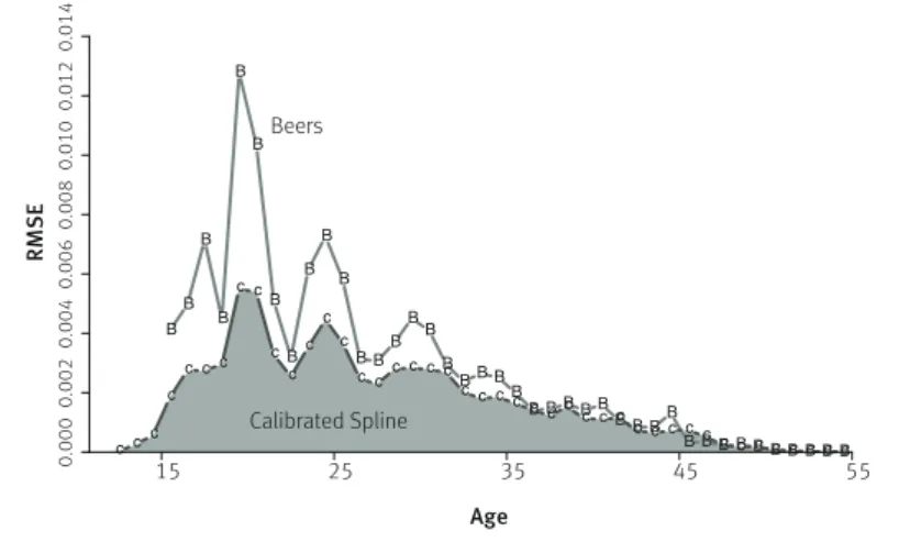
Moving from a single example to a global summary, Graph 5 summarizes the errors for the two methods over all 586 HFD schedules with known single-year rates, disaggregated by age. Notice:
• the vertical scale shows that average errors are very small for both methods;
• the sawtooth pattern of errors at ages below 35 shows that both interpolation methods it single-year data better in the middle of ive-year intervals than they do at the edges. This is an arithmetical property of interpolation when the underlying curve is approximately linear over ive-year intervals: both the itted and true schedules are likely to be close to the age-group average at the center of the age range;
• the pattern of comparative errors by age seen for Scotland 2004 in Graph 4 holds up across all schedules: calibrated spline its are much better at ages below 40, while Beers its (ater ixing negative values) are slightly better at ages above 40;
GRAPH 5
Root mean squared itting errors by age. Calculated over HFD cells with original (rather than estimated) single-year rates B B B B B B B B B B B B B B B B B BB B
B B BBB B
B B B
B
B B B B B B B B B B cc
c c
c cc c c c c c c c
c cc c c cc c c c
c cc c c c
c c c c c
c c c c c c c c
Age
RMSE
15 25 35 45 55
0.000 0.002 0.004 0.006 0.008 0.010 0.012 0.014 Calibrated Spline Beers
Source: HFD (2012).
It is also useful to summarize errors over diferent dimensions. Graph 6 ofers a second global comparison of the methods, this time aggregating over ages and showing the average RMSE by country. Average interpolation errors are lower for the CS method in all 20 populations. Once again, both methods perform very well, but the CS method its better than Beers.
GRAPH 6
Root mean squared itting errors by country. Calculated over HFD cells with original (rather than estimated) single-year rates. Abbreviations from HFD
RMSE
X X X X
X X X
X X X X X X X X X
X X X X 0.000 0.002 0.004 0.006 DEUTE
RUS CZE SVK EST LTU FRA
TNP GBR
TENW NLD SVN GBR_SCO
FIN USA SWE DEUTNP HUN AU T CHE DEUTW GBR _NP B B B B B B B B B B B B
B B B B B B B B Calibrated Spline Beers
Source: HFD (2012).
rather than from a splitting algorithm. The CS method performs better overall, but at high maternal ages its its are slightly worse than those of the adjusted Beers algorithm.
Section B reports measures of the roughness or wiggliness of interpolated schedules, summarizing second diferences by age (1fx+2 - 1fx+1) - (1fx+1 - 1fx) with root mean squared values
(.104) across models it to all 1480 HFD schedules (interpolation from g=9 age groups) and all
226 IDB schedules (g=7). Lower index values in Section B correspond to sets of interpolated schedules with fewer up-and-down wiggles and fewer local maxima in the interpolated single-year rates. Again the CS method performs better, producing smoother schedules.
Section C of Table 1 includes information on a performance criterion for which the CS method is inferior to the (adjusted) Beers approach: negative rate estimates. With the test data at hand, each method produces 1706x43=73358 single-year rate estimates. In the original Beers approach (not shown in the table) approximately 12% of the estimates are negative and 3% are below -.005. However, the Liu et al. variant used here eliminates all negative values through a post-processing algorithm.
TABLE 1
Error summaries for alternative interpolation methods
Beers Calibrated spline
A. Fitting errors (RMSE x 104)
All Ages 42 24
12-24 72 34
25-34 36 26
35+ 11 9
B. Roughness of itted schedule (root mean squared 2nd diference x 104)
HFD (g=9) 76 38
IDB (g=7) 61 43
C. Negative values
(percent of all estimated rates)
< 0 0 2.7
< -.0005 0 0.4
< -.0050 0 0.0+
Source: HFD (2012) and Schmertmann (2003: Supplemental File III).
Note: RMSEs calculated over cells with known single-year data. All other calculations refer to interpolated its over ages 12-54 from all 1706 available 5fx schedules (1480 in HFD + 226 in IDB). Shaded cells correspond to the best- performing method for each error criterion.
In contrast, without adjustment 2.7% of the CS-estimated fertility rates are negative. Although this is of course logically impossible, the vast majority of these negative CS rate estimates are negligibly diferent from zero. As seen in Section C, only 0.4% of CS rates are below -.0005 (i.e., negative ater rounding to three decimal places). In practice, CS estimates are suiciently close to zero that their direct use in calculations such as TFR, mean age of childbearing, etc. would cause no meaningful problems.
However, it is possible to use a very simple post-processing procedure on CS rates – namely,
ater calculating f*=KW y, replace any negative values with zeroes. This is computationally much simpler than the Liu et al. (2011) post-processing algorithm for Beers rates, and it would not alter any of the values in Sections A or B of Table 1.11
In sum, both methods are very good, but the CS method performs slightly better – over all HFD countries, and over the ages at which fertility rates are highest. Interpolated CS schedules are smoother and it known data better. CS calculation is also much simpler than the Beers variant used by Liu et al. (2011), because it does not require complex adjustments for edge efects and negative values.
Discussion
I have presented applications of the calibrated spline model for only two speciic cases, but the general framework is extremely flexible. In principle one can construct expansion constants K that map input data from any set of age groups onto any ine grid of ages. The input age groups may be incomplete (e.g., {25-29,35-39,40-44,45-54}), irregularly spaced ({12-14,15-19,20-24,25-34,…}), or even overlapping ({15-17,15-24,…}).12
The CS model its observed schedules well, outperforming an alternative method that has done well in earlier research. It is also much simpler to estimate. Given the K constants (which in most cases are the ones already provided in this paper and the accompanying data iles), itting a detailed ASFR schedule requires only basic arithmetic. Unlike the Beers method and other generic polynomial itting methods that are not designed speciically for fertility estimation, post-estimation tweaks for negative itted rates at the highest and lowest maternal ages are rarely necessary.
Although not explicitly Bayesian, the CS estimation approach makes heavy use of a priori
information. The penalized least squares criterion gives priority to fertility schedules that not only it input data well, but that also match historical or contemporary patterns seen in large databases. The technique of identifying such patterns through singular value decomposition of a large data array is not new in demography (for example, it is the basis of the Lee-Carter [1992] mortality model), but to my knowledge researchers have not previously used such patterns in a simple, least-squares method like that presented here.
References
BOOR, C. de. A practical guide to splines. New York: Springer-Verlag, 1978.
EILERS, P. H. C.; MARX, B. D. Flexible smoothing using b-splines and penalized likelihood. Statistical Science, v. 11, p. 89-121, 1996.
11 With truncation at zero, the Calibrated Spline column of Table 1 would remain unchanged, except that the percentages in Section C would all be zero.
HFD – Human Fertility Database. Max Planck Institute for Demographic Research and Vienna Institute of Demography, 2012. Available at: <http://www.humanfertility.org>.
HMD – Human Mortality Database. University of California, Berkeley and Max Planck Institute for Demographic Research, 2014. Austrian exposure data at: <http://www.mortality.org/hmd/AUT/STATS/ Exposures_5x1.txt>. Accessed: 14 Nov. 2014.
IBGE – Instituto Brasileiro de Geograia e Estatística. Censo Demográico do Brasil. Rio de Janeiro, 2010.
LEE, R. D.; CARTER, L. R. Modeling and forecasting U.S. mortality. Journal of the American Statistical Association, v. 87, n. 419, p. 659-671, 1992.
LIU, Y.; GERLAND, P.; SPOORENBERG, T.; VLADIMIRA, K.; ANDREEV, K. Graduation methods to derive age-speciic fertility rates from abridged data: a comparison of 10 methods using HFD data. In: FIRST HUMAN FERTILITY DATABASE SYMPOSIUM. Rostock: Max Planck Institute for Demographic Research, November 2011. Available at: <http://www.humanfertility.org/Docs/Symposium/Liu-Gerland%20et%20 al.pdf>. Accessed: 10 Jun. 2012.
MPC – Minnesota Population Center. Integrated public use microdata series, international: version 6.3 [Machine-readable database]. Minneapolis: University of Minnesota, 2014.
NRS – National Records of Scotland. Estimated population by sex and age, Scotland, 30 June 2004. 2014. Available at: <http://goo.gl/1F7ANk>. Accessed: 14 Nov. 2014.
R DEVELOPMENT CORE TEAM. R: A language and environment for statistical computing. Vienna: R Foundation for Statistical Computing, 2011. Available at: <http://www.R-project.org>.
SCHMERTMANN, C. P. A system of model fertility schedules with graphically intuitive parameters.
Demographic Research, v. 9/5, p. 81-110, 2003. Available at: <http://dx.doi.org/10.4054/ DemRes.2003.9.5>.
SHRYOCK, H. S.; SIEGEL, J. S. The methods and materials of demography. Third printing (rev.). Washington DC: US Bureau of the Census, US Government Printing Oice, v. 2, 1975.
UNSD – United Nations Statistics Division. Female population of Uruguay 2002. 2014. Available at: <http://goo.gl/DMKMNc>. Accessed: 11 Nov. 2014.
Author
Carl P. Schmertmann is Doctor in Economics from the University of California – Berkeley, researcher in Demography and Professor of Economics at Florida State University.
Address
FSU Population Center 601 Bellamy Building 113 Collegiate Loop
Resumo
Estimadores splines calibrados: estimativas de taxas detalhadas de fecundidade a partir de dados agrupados por idade
É desenvolvido e explicado um novo método para a interpolação de estruturas etárias detalhadas de fecundidade, a partir de dados agrupados por idade. O método permite a estimativa das taxas especíicas de fecundidade para qualquer idade detalhada, desde as diferentes faixas etárias padrão até qualquer agrupamento não usualmente utilizado. O novo método, chamado de estimador spline calibrado (CS), expande as taxas de fecundidade agrupadas por idade encontrando uma curva suavizada, por minimização dos erros quadrados penalizados. A penalidade é baseada tanto no ajuste aos dados dos grupos etários disponíveis, quanto na semelhança dos padrões das estruturas etárias 1fx observadas no Banco Human Fertility Database (HFD) e no US Census International Database (IDB). O estimador CS foi comparado a um bom método alternativo que requer mais computação: interpolação de Beers. Os resultados mostram que o CS replica as conhecidas estruturas etárias de fecundidade, 1fx, a partir das 5fx melhoradas, sendo que as estruturas etárias da fecundidade interpoladas apresentam-se também mais suavizadas. A conclusão é que o CS constitui um método facilmente calculado, flexível e preciso para a interpolação de estruturas de fecundidade detalhadas a partir de dados agrupados. Os usuários podem calcular estruturas especíicas de fecundidade detalhadas diretamente por meio dos dados observados, usando apenas aritmética elementar.
Palavras-chave: Fecundidade. Interpolação. Splines. Mínimos quadrados penalizados.
Resumen
Estimadores spline calibrados para tasas detalladas de fecundidad a partir de datos agrupados por edad
Se desarrolla y explica un nuevo método para la interpolación de estructuras etarias detalladas de fecundidad a partir de datos agrupados por edad. El método permite la estimación de las tasas especíicas de fecundidad para cualquier edad detallada, desde los diferentes segmentos etarios estándar hasta cualquier agrupamiento no utilizado usualmente. El nuevo método, llamado estimador spline calibrado (CS), expande las tasas de fecundidad agrupadas por edad encontrando una curva suavizada mediante la minimización de los errores cuadrados penalizados. La penalización se basa tanto en el ajuste de los datos de los grupos etarios disponibles como en la semejanza de los patrones de las estructuras de edad 1fx observados en la Human Fertility Database (HFD) y la US Census International Database (IDB). El estimador CS se comparó con un buen método alternativo que requiere más procesamiento: la interpolación de Beers. Los resultados muestran que el CS replica las conocidas estructuras etarias de fecundidad 1fx, a partir de las 5fx mejoradas, donde las estructuras etarias de la fecundidad interpoladas también se presentan más suavizadas. La conclusión a la que se arriba es que el CS constituye un método fácil de calcular, flexible y preciso para la interpolación de estructuras de fecundidad detalladas a partir de datos agrupados. Los usuarios pueden calcular estructuras especíicas de fecundidad detalladas directamente por medio de los datos observados, solo utilizando la aritmética elemental.
Appendix: Moment calculations from age group data
One possible use of the empirical model is estimation of moments of the continuous fertility schedule from grouped data. This type of approximation might be especially useful with indirect methods.
Begin by deining the function:
∫
= x n
n x a a da
Q
α φ( )
) (
(A1) which can be approximated as
y x c y b a y b a f a a a x Q n W W x a i i n i W W x a i i n i x a i i n i x a i i n i n i i i i ) ( ) ( ) ( 1 : 1 : : : ʹ = ⎟ ⎟ ⎠ ⎞ ⎜ ⎜ ⎝ ⎛ Δ ʹ = Δ ʹ = Δ = Δ ≈ − < − < < <
∑
∑
∑
∑
R Q R Q φ (A2)Where QW and RW are deined as in equations (12) and (13), and cn(x) is therefore a g x 1
vector of known constants.
With diferent (x,n) combinations, Equation (A2) produces diferent moments of the fertility function. Table A1 shows some of the calculated constants for the g=7 case; a more complete set of constants, calculated using the suggested default of W=1000, is available in supplemental ile Cdata.csv.
By deinition Q0(∞) is a schedule’s total fertility (TFR), and Q1(∞)/Q0(∞) is its mean age of childbearing μ. In the case of the Uruguay 2002 data shown earlier, for example, we can approximate these quantities as:
TFR = Q0(∞) ≈ 3.44(.049) + … + 0.66(.002) = 2.328
μ = Q1(∞) / Q0(∞) ≈ [60.78(.049) + … + 27.15(.002)] / 2.328 = 28.23
Similarly, one can approximate conditional moments such as average parity of women 30-34 [Q0(32.5)] and the average age at which they had their previous births [Q1(32.5)/ [Q0(32.5)]. With the Uruguay data these moments would be:
P30-34 ≈ Q0(32.5) ≈ 3.51(.049) + … -0.03 (.002) = 1.753
μ30-34 ≈ Q1(32.5) / Q0(32.5) ≈ [63.46(.049) + … -1.53(.002)] / 1.753 = 25.37
TABLE 1
Some c multipliers for the g=7 case
15-19 20-24 25-29 30-34 35-39 40-44 45-49
n=0 (TFR)
x = 17.5 1.06 -0.09 -0.03 0.08 0.02 0.15 0.08
x = 22.5 3.78 3.12 -0.53 -0.02 -0.07 -0.06 0.02
x = 27.5 3.48 5.86 2.37 -0.19 -0.18 0.01 0.01
x = 32.5 3.51 5.49 5.12 2.58 0.06 -0.38 -0.03
x = 37.5 3.53 5.31 5.32 4.91 2.23 0.53 0.09
x = 42.5 3.40 5.43 4.97 5.32 4.63 2.55 0.40
x = 47.5 3.44 5.38 4.84 5.34 5.45 3.53 0.63
x = ∞ 3.44 5.38 4.83 5.34 5.48 3.57 0.66
n=1 (TFR ∙ μ)
x = 17.5 17.12 -1.44 -0.39 1.29 0.23 2.28 1.18
x = 22.5 70.24 65.04 -10.41 -0.98 -1.43 -1.84 0.07
x = 27.5 62.45 131.62 63.76 -4.59 -4.38 -0.36 -0.21
x = 32.5 63.46 120.12 144.93 79.44 3.43 -11.92 -1.53
x = 37.5 64.12 114.23 151.35 160.02 79.96 20.88 2.89
x = 42.5 59.04 118.92 137.37 176.23 175.54 101.65 15.51
x = 47.5 60.70 116.70 131.64 177.09 211.81 145.18 25.68
x = ∞ 60.78 116.63 131.32 177.13 213.45 147.07 27.15
Source: Author’s calculations based on Equation (A2).