A Work Project, presented as part of the requirements for the award of a Masters Degree in
Finance from the Faculdade de Economia da Universidade Nova de Lisboa.
The Impact of Foreign Currency Debt on
Credit Risk
Analyzing Exchange Rate Risk in International Credit Markets
-Supplementary Appendix-
January 6
th, 2017
Nadja Christina Merz
Arellano-Bond Difference GMM
The difference GMM estimator following Arellano and Bond (1998) is designed for panels
with many groups and few periods, where the model describes a linear relationship between a
dynamic dependent variable and explanatory variables. Furthermore, the estimation allows for
time-invariant fixed effects and heteroskedasticity as well as autocorrelation within countries.
When compared to standard OLS techniques, the main advantage of difference GMM is that
it allows for endogenous as well as predetermined variables in the context of a dynamic
model.
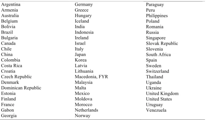
Equation (1.a), (1.b) and (2.a), (2.b) describe the models to be estimated in this paper,
covering a sample of 62 countries over the period 2000 to 2014.
𝑁𝑃𝐿$,&= 𝛽)+ 𝛽+𝑁𝑃𝐿$,&,++ 𝛽-𝑅𝐸𝐸𝑅$,&+ 𝛽0𝐼𝐶$,&+ 𝛽3 𝑅𝐸𝐸𝑅$,&∙ 𝐼𝐶$,& + 𝛽5𝑋$,&7 + 𝜇$+ 𝜀$,& (1.a)
𝑁𝑃𝐿$,&= 𝛽)+ 𝛽+𝑁𝑃𝐿$,&,++ 𝛽-𝑅𝐸𝐸𝑅$,&+ 𝛽0𝐼𝐶$,&+ 𝛽3 𝑅𝐸𝐸𝑅$,&∙ 𝐼𝐶$,& ∙ ℎ𝑖𝑔ℎ𝐼𝐶$,&+
𝛽5 𝑅𝐸𝐸𝑅$,&∙ 𝐼𝐶$,& ∙ 𝑙𝑜𝑤𝐼𝐶$,&+ 𝛽F𝑋$,&7 + 𝜇$+ 𝜀$,&
(1.b)
𝑁𝑃𝐿$,&= 𝛽)+ 𝛽+𝑁𝑃𝐿$,&,++ 𝛽-𝑉_𝑅𝐸𝐸𝑅$,&+ 𝛽0𝐼𝐶$,&+ 𝛽3 𝑉_𝑅𝐸𝐸𝑅$,&∙ 𝐼𝐶$,& + 𝛽5𝑋$,&7 + 𝜇$+ 𝜀$,& (2.a)
𝑁𝑃𝐿$,&= 𝛽)+ 𝛽+𝑁𝑃𝐿$,&,++ 𝛽-𝑉_𝑅𝐸𝐸𝑅$,&+ 𝛽0𝐼𝐶$,&+ 𝛽3 𝑉_𝑅𝐸𝐸𝑅$,&∙ 𝐼𝐶$,& ∙ ℎ𝑖𝑔ℎ𝐼𝐶$,&+
𝛽5 𝑉_𝑅𝐸𝐸𝑅$,&∙ 𝐼𝐶$,& ∙ 𝑙𝑜𝑤𝐼𝐶$,&+ 𝛽F𝑋$,& 7
+ 𝜇$+ 𝜀$,& (2.b)
The Arellano and Bond (1991) estimation is based on the following orthogonality conditions
that apply to all four specifications (Bun and Windmeijer, 2010; Bond, Hoeffler and Temple,
2001):
E NPLO,P,Q ΔεO,P = 0 for t = 2002, … , T and 2001 ≤ s ≤ T − 1;
(GMM.1)
𝑍$ =
𝑁𝑃𝐿$,+ 0 0 … 0 … 0
0 𝑁𝑃𝐿$,+ 𝑁𝑃𝐿$,- … 0 … 0
. . . … . . .
0 0 0 … 𝑁𝑃𝐿$,+ … 𝑁𝑃𝐿
$,c,-(GMM.2)
Condition (GMM.1) implies that lagged levels of date
(t − 2)
and earlier may be employed as
valid instruments for the model in first differences (Arellano and Bond, 1991).
The rationale towards endogenous explanatory variables follows a similar intuition. Let
x
O,Pdenote an endogenous variable in the specification. The moment condition can be written
as:
E xO,P,Q ΔεO,P = 0 for t = 2001, … , T and 1 ≤ s ≤ T − 1
(GMM.4)
GMM.4 implies that lagged values of endogenous variables may validly be used as
instruments for contemporaneous values.
In order to verify the validity of the approach, all estimations include the Arellano-Bond test
for autocorrelation of order one and two (Arellano and Bond, 1991). Basically, the
differenced error term must be uncorrelated to the second and higher lags of the dependent
variable:
E NPLO,P,e ΔεO,P = 0 for j ≥ 2
(GMM.5)
If the condition above were not to hold, endogeneity would again bias the estimates.
Therefore, a valid specification must not reject the null hypothesis of no autocorrelation of
order two and higher.
Moreover, a Sargan-Test is employed to test the validity of instruments (Arellano and Bond,
1991). Following an asymptotic
χ
-- distribution, the test assesses the overidentifying
restrictions implied by the instrument matrices (GMM.2) and (GMM.4). In order to prove the
power of the instruments, the test must not reject the null of instrument validity. However, too
many instruments can easily over-fit endogenous variables, leading to unrealistically high
In order to verify the assumption of mean stationarity, Augmented Dickey-Fuller unit-root
tests as well as Im-Persean-Shin tests were performed (Dickey and Fuller, 1981; Im, Persean
and Shin, 2003).
Lastly, I calculate a pseudo
R
-to measure the fit of model, calculated as the squared
correlation of actual values and fitted values of the dependent variable.
𝑝𝑠𝑒𝑢𝑑𝑜 𝑅- = 𝑐𝑜𝑟𝑟(NPLO,P, NPLq,P)-
(GMM.6)
The most important criteria when assessing the validity of the model, however, are
Table A.2
Data Sources
Indicator Sources
Non-performing loans •World Bank –Word Development Indicators
Real Effective Exchange Rate •Bank of International Settlements – BIS effective exchange rate indices (broad indices)
•International Monetary Fund – International Financial Statistics
International Claims •Bank of International Settlements – Consolidated Banking Statistics (A – All reporting banks, A – International claims; cross-border claims in all currencies and local claims in non-local currencies)
Real Gross Domestic Product •World Bank –Word Development Indicators
Lending Interest Rate •World Bank –Word Development Indicators
Trade •World Bank –Word Development Indicators
Unemployment •World Bank –Word Development Indicators
Banking Crisis Dummy •World Bank - Global Financial Development Database
Financial Market Development •World Economic Forum’s Global Competitive Index Historical Dataset
Table A.3
Institute of International Finance Loan Classification Scheme
Loan Category Definition
Standard Credit is sound and all principal and interest payments are current. Repayment
difficulties are not foreseen under current circumstances and full repayment is expected.
Watch Asset subject to conditions that, if left uncorrected, could raise concerns about full
repayment. These require more than normal attention by credit officers.
Substandard Full repayment is in doubt due to inadequate protection (e.g., obligor net worth or
collateral) and/or interest or principal or both are more than 90 days overdue. These assets show underlying, well- defined weaknesses that could lead to probable loss if not corrected and risk becoming impaired assets.
Doubtful Assets for which collection/liquidation in full is determined by bank management
to be improbable due to current conditions and/or interest or principal or both are overdue more than 180 days. Assets in this category are considered impaired, but are not yet considered total losses because some pending factors may strengthen the asset’s quality (merger, new financing, or capital injection).
Loss An asset is downgraded to loss when management considers the facility to be
virtually uncollectible and/or principal or interest or both are overdue more than one year.
Source: Krueger (2002)
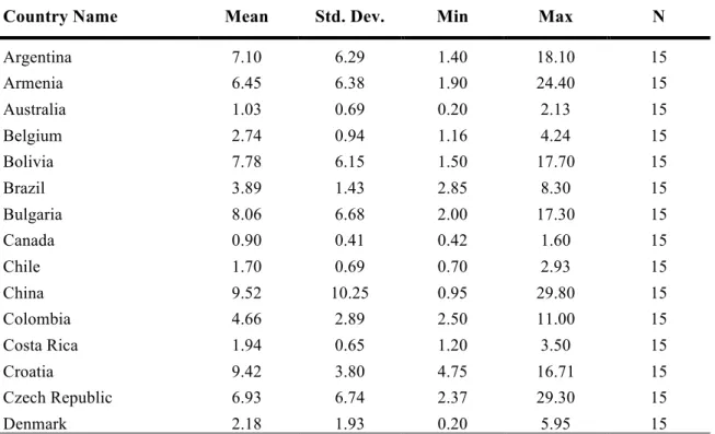
Table A.4
Descriptive Statistics of NPL Ratios
Country Name Mean Std. Dev. Min Max N
Argentina 7.10 6.29 1.40 18.10 15
Armenia 6.45 6.38 1.90 24.40 15
Australia 1.03 0.69 0.20 2.13 15
Belgium 2.74 0.94 1.16 4.24 15
Bolivia 7.78 6.15 1.50 17.70 15
Brazil 3.89 1.43 2.85 8.30 15
Bulgaria 8.06 6.68 2.00 17.30 15
Canada 0.90 0.41 0.42 1.60 15
Chile 1.70 0.69 0.70 2.93 15
China 9.52 10.25 0.95 29.80 15
Colombia 4.66 2.89 2.50 11.00 15
Costa Rica 1.94 0.65 1.20 3.50 15
Croatia 9.42 3.80 4.75 16.71 15
Czech Republic 6.93 6.74 2.37 29.30 15
Denmark 2.18 1.93 0.20 5.95 15
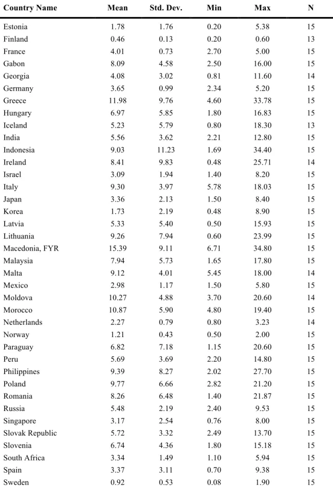
Table A.4
Descriptive Statistics of NPL Ratios (continued)
Country Name Mean Std. Dev. Min Max N
Estonia 1.78 1.76 0.20 5.38 15
Finland 0.46 0.13 0.20 0.60 13
France 4.01 0.73 2.70 5.00 15
Gabon 8.09 4.58 2.50 16.00 15
Georgia 4.08 3.02 0.81 11.60 14
Germany 3.65 0.99 2.34 5.20 15
Greece 11.98 9.76 4.60 33.78 15
Hungary 6.97 5.85 1.80 16.83 15
Iceland 5.23 5.79 0.80 18.30 13
India 5.56 3.62 2.21 12.80 15
Indonesia 9.03 11.23 1.69 34.40 15
Ireland 8.41 9.83 0.48 25.71 14
Israel 3.09 1.94 1.40 8.20 15
Italy 9.30 3.97 5.78 18.03 15
Japan 3.36 2.13 1.50 8.40 15
Korea 1.73 2.19 0.48 8.90 15
Latvia 5.33 5.40 0.50 15.93 15
Lithuania 9.26 7.94 0.60 23.99 15
Macedonia, FYR 15.39 9.11 6.71 34.80 15
Malaysia 7.94 5.73 1.65 17.80 15
Malta 9.12 4.01 5.45 18.00 14
Mexico 2.98 1.17 1.50 5.80 15
Moldova 10.27 4.88 3.70 20.60 14
Morocco 10.87 5.90 4.80 19.40 15
Netherlands 2.27 0.79 0.80 3.23 14
Norway 1.21 0.43 0.50 2.00 15
Paraguay 6.82 7.18 1.15 20.60 15
Peru 5.69 3.69 2.20 14.80 15
Philippines 9.39 8.27 2.02 27.70 15
Poland 9.77 6.66 2.82 21.20 15
Romania 8.26 6.48 1.40 21.87 15
Russia 5.48 2.19 2.40 9.53 15
Singapore 3.17 2.54 0.76 8.00 15
Slovak Republic 5.72 3.32 2.49 13.70 15
Slovenia 6.74 4.36 1.80 15.18 15
South Africa 3.34 1.49 1.10 5.94 15
Spain 3.37 3.11 0.70 9.38 15
Sweden 0.92 0.53 0.08 1.90 15
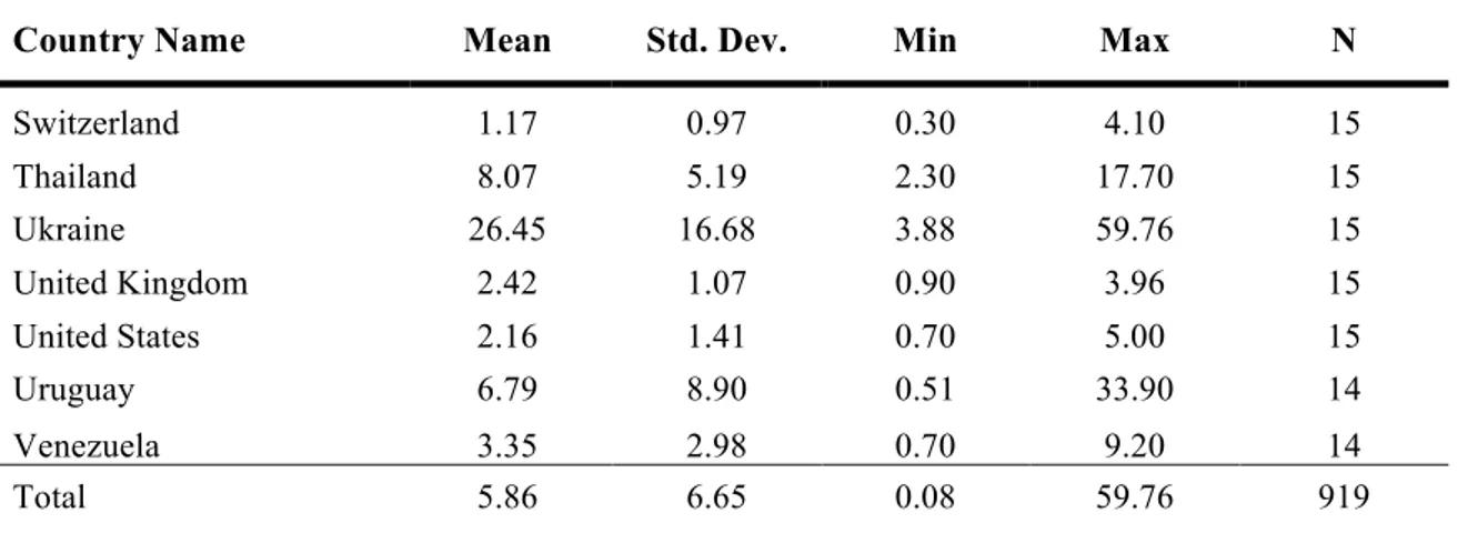
Table A.4
Descriptive Statistics of NPL Ratios (continued)
Country Name Mean Std. Dev. Min Max N
Switzerland 1.17 0.97 0.30 4.10 15
Thailand 8.07 5.19 2.30 17.70 15
Ukraine 26.45 16.68 3.88 59.76 15
United Kingdom 2.42 1.07 0.90 3.96 15
United States 2.16 1.41 0.70 5.00 15
Uruguay 6.79 8.90 0.51 33.90 14
Venezuela 3.35 2.98 0.70 9.20 14
Total 5.86 6.65 0.08 59.76 919
N represents the number of available data points. NPLs statistics are based on annual data between 2010-2014. Source: World Bank and author’s calculations
Figure A.1
Growth of NPL Ratio (%)
Source: World Bank and author’s calculations
-0,4 -0,2 0 0,2 0,4 0,6 0,8 1 1,2 1,4
2000 2001 2002 2003 2004 2005 2006 2007 2008 2009 2010 2011 2012 2013 2014
Table A.5
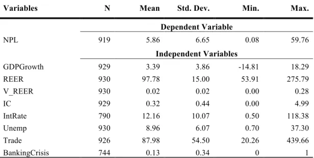
Selected Descriptive Statistic
Variables N Mean Std. Dev. Min. Max.
Dependent Variable
NPL 919 5.86 6.65 0.08 59.76
Independent Variables
GDPGrowth 929 3.39 3.86 -14.81 18.29
REER 930 97.78 15.00 53.91 275.79
V_REER 930 0.02 0.02 0.00 0.28
IC 929 0.32 0.44 0.00 4.99
IntRate 790 12.16 10.07 0.50 118.38
Unemp 930 8.96 6.07 0.70 37.30
Trade 926 87.98 54.50 20.26 439.66
BankingCrisis 744 0.13 0.34 0 1
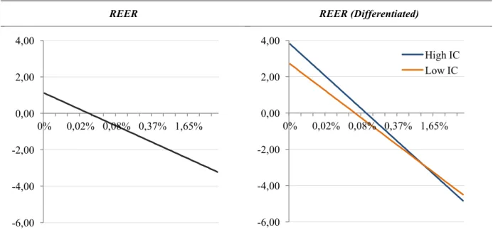
Figure A.2
Marginal Effects of Exchange Rate Movements on NPLs Conditional on
Different Levels of International Claims
REER REER (Differentiated)
V_REER V_REER (Differentiated)
The vertical axis shows the percentage change of the growth rate of non-performing loans given a percentage change in REER or V_REER; the horizontal axis shows the ratio of international claims to GDP on a logarithmic scale.
-6,00 -4,00 -2,00 0,00 2,00 4,00
0% 0,02% 0,08% 0,37% 1,65%
-6,00 -4,00 -2,00 0,00 2,00 4,00
0% 0,02% 0,08% 0,37% 1,65% High IC Low IC
-40 -20 0 20 40
0% 0,02% 0,08% 0,37% 1,65%
-40 -20 0 20 40
0% 0,02% 0,08% 0,37% 1,65%
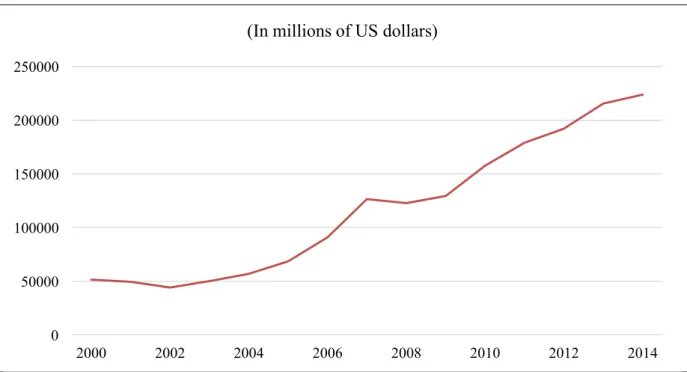
Figure A.3
Average International Claims of Emerging Markets
Source: BIS consolidated banking statistics and author’s calculations
Table A.6
List of Emerging Markets including in the subsample
ArgentinaBrazil Chile China Colombia Czech Republic Hungary
India Indonesia Israel Malaysia Mexico Peru Philippines
Poland Romania Russia South Africa Thailand Ukraine Venezuela 0
50000 100000 150000 200000 250000
2000 2002 2004 2006 2008 2010 2012 2014
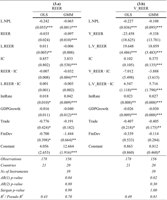
Table A.7
Determinants of NPLs – Emerging Markets
(3.a)REER
(3.b) V_REER
OLS GMM OLS GMM
L.NPL -0.242 -0.065 L.NPL -0.227 -0.108
(0.055)*** (0.081)*** (0.036)*** (0.095)***
REER -0.035 -0.097 V_REER -23.458 -9.338
(0.024) (0.010)*** (18.625) (13.781)
L.REER 0.011 -0.006 L.V_REER 19.648 18.059
(0.005)** (0.008) (4.486)*** (5.483)***
IC 0.857 3.833 IC 0.102 0.375
(0.802) (0.538)*** (0.105) (0.135)*** REER∙ IC -0.007 -0.032 V_REER∙ IC -7.012 -3.888
(0.008) (0.004)*** (5.498) (3.615) L.REER∙ IC 0.001 -0.003 L.V_REER ∙IC 6.547 5.716
(0.001) (0.002) (1.118)*** (1.798)***
IntRate 0.018 0.042 IntRate 0.023 0.027
(0.010)* (0.009)*** (0.008)** (0.008)*** GDPGrowth -0.016 -0.040 GDPGrowth -0.026 -0.030
(0.011) (0.012)*** (0.009)*** (0.008)***
Trade -0.776 -0.191 Trade -0.407 -0.405
(0.424)* (0.182) (0.218)* (0.175)**
FinDev -0.700 -1.444 FinDev -0.339 -0.114
(0.398)* (0.664)** (0.533) (0.284)
Constant 4.056 12.664 Constant 0.863 0.812
(2.653) (1.916)*** (0.860) (0.460)*
Observations 178 156 178 156
Countries 21 20 21 20
No of Instruments 39 39
AR(1) p-value 0.04 0.02
AR(2) p-value 0.80 0.30
Sargan p-value 0.99 1.00
R2 / Pseudo R2 0.43 0.70 0.49 0.81
The dependent variable is the first difference of NPLs in natural logarithm. Standard Errors in parentheses.
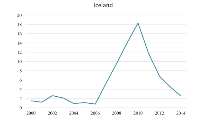
Figure A.4
Non-Performing Loans ratio (%) of Iceland
Source: World Bank - Word Development Indicators
0 2 4 6 8 10 12 14 16 18 20
2000 2002 2004 2006 2008 2010 2012 2014
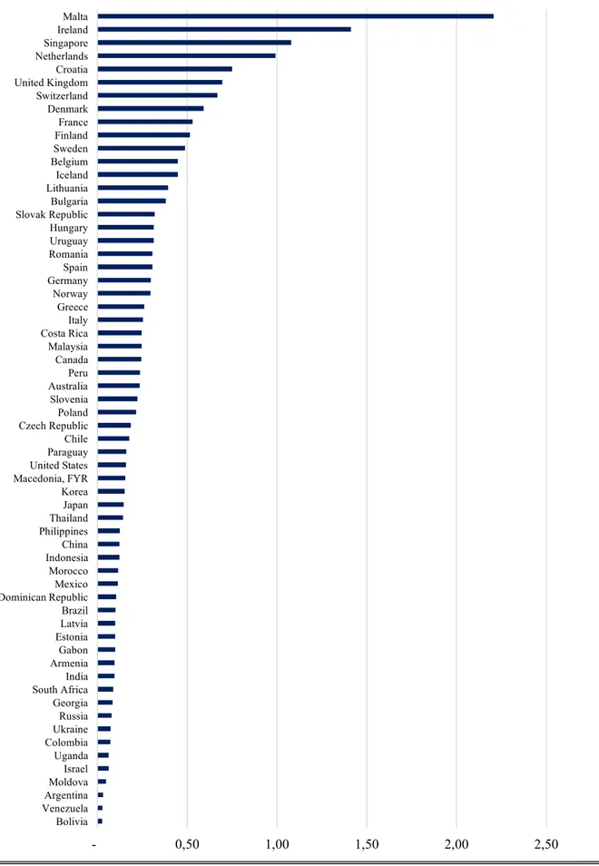
Figure A.5
International Claims relative to GDP in 2014
Source: Bank of International Settlement and author’s calculation
- 0,50 1,00 1,50 2,00 2,50
Table A.8
List of Abbreviations
BCBS Basel Committee for Banking Supervision BIS Bank of International Settlements
CDS Credit Default Swaps
GDP Gross domestic product
GMM Generalized method of moments
IC International claims
IMF International Monetary Fund IntRate Lending interest rate
LLP Loan loss provisions
NPLs Non-performing loans
OLS Ordinary Least Squares REER Real effective exchange rate
Unemp Unemployment