A Work Project, presented as part of the requirements for the award of a Masters Degree in Finance from the Faculdade de Economia da Universidade Nova de Lisboa.
The Impact of Foreign Currency Debt on
Credit Risk
Analyzing Exchange Rate Risk in International Credit Markets
A project carried out under the supervision of: Professor André Castro Silva
January 6th, 2017
The Impact of Foreign Currency Debt on
Credit Risk
Analyzing Exchange Rate Risk on International Credit Markets
Abstract
This paper identifies the role of exchange rate movements as well as exchange rate volatility as determinants of non-performing loans (NPLs) using panel data across 62 countries from 2000 to 2014. Dynamic panel data estimations suggest that a depreciation of the domestic currency has a negative effect on NPLs: The results indicate that negative balance sheet effects generally outweigh gains in competitiveness in international markets. Exchange rate volatility, as a measure of uncertainty towards exchange rate movements, has a statistically significant and strong impact on default ratios. The estimation technique accounts for possible concerns of endogeneity, reverse causality and omitted variable bias. The results are robust to various specifications and a subsample of emerging markets only.
JEL classification:C33, F31, F34, F36, G15, G32, P33
Keywords: Credit risk; non-performing loans; currency mismatch; exchange rate; exchange rate volatility; dynamic panel estimation
Acknowledgements
1 Introduction
This paper sets out to investigate the empirical determinants of the non-performing loan (NPLs) ratio as a measure of credit risk using linear dynamic panel estimations, based on a sample of 62 countries over the years 2000-2014. In addition to standard empirical determinants of bank asset quality, I analyze the effects of real effective exchange rate movements as well as uncertainty towards the exchange rate, i.e. exchange rate volatility, on credit risk conditional on foreign currency debt levels.
Credit risk is tightly associated with financial stability throughout the world. The financial crisis in 2007-2008 has proven the need to readjust the common methodology used in identifying and addressing credit risk, as the average bank asset quality deteriorated sharply during the economic recession (Beck, Jakubik and Piloiu, 2015). Studying the determinants of credit risk and establishing an early warning system is a major concern of financial institutions and supervisory bodies around the globe. In the literature, credit risk is defined as “the risk of changes in credit portfolio value associated with unexpected changes in credit quality (“mark-to-market” approach) or, alternatively, the risk of unexpected losses stemming from counterpart defaults (“default mode” approach)” (Virolainen 2004, 8).
fact, many economies have become highly dependent on capital inflows as well as foreign credit over the last decade.
Nevertheless, debt issued in foreign currency exposes borrowers not only to rollover risk and sudden capital flow reversals but also to significant foreign currency risks (European Central Bank, 2016). Countries that face high foreign currency liabilities that are not offset by foreign currency assets, i.e. countries that face currency mismatches, are particularly exposed to exchange rate risks (Bordo and Meissner, 2006). As foreign-currency markets have suddenly become more volatile due to the divergence in monetary policy across the globe as well as falling commodity prices, many countries saw these risks materializing in recent years. Increasing capital costs and tightened funding conditions following the recent normalization of the US American monetary policy are likely to further impede economic activity in emerging markets and raise the pressure on exchange rates.
Understanding the role of exchange rate movements and exchange rate volatility in the context of foreign currency denoted debt supports the identification of key vulnerabilities in the banking system. This paper establishes an empirical perspective to evaluate the gravity of exchange rate risks and helps to refine existing stress tests based on macro-prudential surveillance.
2 Literature Review
The determinants of NPLs as a proxy for credit risk, i.e. the quality of bank assets, have been under thorough investigation, especially after the financial crisis. The measures of credit risk, however, differ widely in the literature. Among the measures that are used the most are loan loss provisions (LLP) and Credit Default Swaps (CDS) spreads and non-performing loan ratios. According to Glen and Mondragón-Vélez (2011), based on a panel of 22 advanced economies during the period 1996-2008, LLP are mainly determined by private sector leverage, real GDP growth and a lack of capitalization within the banking system. Studying 26 advanced economies during the period of 1998-2009, Nkusu (2011) finds that increased NPLs are associated with an adverse macroeconomic development. A third important indicator of distress is CDS spreads. Ötker-Robe and Podpiera (2010) find “that Large Complex Financial Institutions’ business models, earnings potential, and economic uncertainty are among the most significant determinants of credit risk” (Ötker-Robe and Podpiera 2010, 24).
generalized method of moments (GMM) method the authors find that in the case of the exchange rate, the effect is higher for countries with a high share of unhedged foreign exchange lending.
It is important to mention that most of the literature is based on country specific studies and therefore many research papers include a composition of micro and macroeconomic factors. Research by Salas and Saurina (2002), for example, compares problem loans of commercial and savings banks in Spain and find microeconomic determinants such as capital ratio, bank size net interest margin and market power to be statistical significant. Louzis et al. (2010) look at the Greek banking sector and find that credit quality (measured by the NPLs ratio) is mainly determined by macroeconomic fundamentals such as GDP, interest rates and unemployment as well as management quality.
3 Empirical Methodology
3.1 Data
This study comprises a panel of 62 countries1 covering the years 2000-2014.2 The dependent variable is the ratio of non-performing loans to total (gross) loans. Among the most commonly used definitions for NPLs are those of the Basel Committee for Banking Supervision (BCBS), the International Monetary Fund (IMF) and the Institute of International Finance. According to the BCBS definition, “a default occurs when the obligor is 90 days past due on any material credit obligation to the banking group, or is unlikely to pay its credit obligations to the banking group in full, without recourse by the bank to actions such as realizing security” (Basel Committee on Banking Supervision 2006, 100). In its Financial Soundness Indicators Compilation Guide the IMF also states that “loans (and other assets) should be classified as NPLs when (1) payments of principal and interest are past due by three months (90 days) or more, or (2) interest payments equal to three months (90 days) interest or more have been capitalized (re-invested into the principal amount), refinanced, or rolled over (i.e. payment has been delayed by arrangement)” (IMF 2006, 46). The Institute of International Finance has developed a credit classification system, which entails the following five categories: “Standard”, “Watch”, “Substandard”, “Doubtful”, and “Loss loans” (Krueger,
2002).3 However, it does not provide numerical thresholds for the various categories but rather sets up a universal guideline.
There are noteworthy differences in the reporting across countries: Besides the number of days overdue, some jurisdictions report the net value of NPLs (after deduction of the provisions) instead of recording in gross terms. Also the treatment of collateral and guarantees for asset classification and provisioning purposes vary widely. Furthermore, there are
1 List of countries in the Appendix (Table A.1). 2
differences when considering only the amount that is overdue of the NPLs, in which case NPLs ratios are significantly biased downward. A further differentiation is whether or not judicial procedures have been started. Since there is no internationally uniform standard for the definition and measurement of NPLs, the reporting varies across countries. Hence, it is necessary to be cautious when making international comparisons.
This paper uses NPLs data available from the World Bank’s World Development Indicators database, which draws upon the IMF’s Financial Stability indicators. In order to reduce the measurement error due to different reporting standards of NPLs among countries, this paper uses the logarithmic differences instead of NPLs levels. A first descriptive look at the NPLs data reveals that for both, advanced economies as well as emerging markets bank asset quality improved until the onset of the crisis.4 However, after the US sub-prime mortgage crisis starting in 2007 hit the global economy, the growth rate of NPLs tremendously jumped to new record levels, clearly showing the impact of the financial crisis.5
The main explanatory variables under inspection are real effective exchange rate (REER) and volatility of the real effective exchange rate (V_REER). This paper focuses on the exchange rate in real terms, calculated as geometric weighted averages of bilateral exchange rates, that capture movements relative to the base year 2010. The data is gathered from the Bank of International Settlements’ (BIS) statistics (with 54 economies included in the panel) and the IMF’s International Financial Statistics (8 economies). The real effective exchange rate volatility is calculated as the annual standard deviation of the first differenced logarithms of monthly real exchange rates. This measure is widely used and has the benefit that in case the exchange rate follows a constant trend it will equal zero. This prevents that exchange rate trends are anticipated and is therefore an adequate measure for uncertainty regarding real effective exchange rate shocks (Clark et al., 2004). The decision between nominal and real
4
exchange rates in the context of the study depends on the time horizon of the repayment schedule of foreign currency loans. In a long-term scenario, the real effective exchange rate is a more appropriate measure to employ, as import and export prices as well as production costs vary. In reality, however, given sticky domestic prices and slow economic adjustment, nominal and real effective exchange rates move closely together (Clark et al., 2004). In this paper, I employ exchange rate movements as well as exchange rate volatility in real terms.
In order to capture the impact of exchange rate dynamics on credit risk, I interact exchange rate as well as exchange rate volatility with a measure of foreign currency lending. Data for loans denominated in foreign currency is rare, therefore international claims are used as a proxy. Beck, Jakubik and Piloiu (2015) find a positive correlation between international claims and foreign currency lending. This paper follows the assumption that foreign currency denoted debt can be approximated by international claims with sufficient precision.6 Hence, high levels of international claims can be used as an indicator of currency mismatches and unhedged foreign currency lending. Data for international claims is available from the BIS and is employed as a percentage of GDP (IC). Further explanatory variables cover country-specific macroeconomic and financial indicators including real GDP growth (GDPgrowth), the unemployment rate (Unemp), trade as the sum of exports and imports to GDP (Trade), and the lending interest rate (IntRate). All these variables are gathered from the World Bank’s World Development Indicators database. Furthermore, a banking crisis dummy
(BankingCrisis) is used, which is obtained from the World Bank Global Financial
Development Database and is based on Laeven and Valencia (2013). Table A.5 in the Appendix provides descriptive statistics of all variables used in this analysis.
6 Total international claims of all BIS reporting banks to the respective country, including local lending in
3.2 Theoretical Model
Among the range of possible mechanisms how REER can affect NPLs, this paper sets out to investigate two channels, which work in opposite directions: On the one hand, one can expect that currency depreciations lead to an increase of NPLs in countries with currency mismatches: Negative balance sheet effects increase the debt servicing costs in local currency terms for unhedged borrowers with debt denominated in foreign currency. This typically causes ‘a fear of floating’ and motivates to hold the exchange rate tightly pegged to the euro or the US dollar among respective governments (Hausmann et al., 2001). On the other hand, exchange rate depreciation can improve the financial position of the corporate sector, particularly in countries with a large export volume. A depreciation of the domestic currency can thus translate into gains in international competitiveness and a reduction of credit default rates (trade effect).
Apart from exchange rate appreciations or depreciations, unforeseen movements of the domestic currency relative to foreign currencies are an important source of uncertainty and risk (Clark et al., 2004). Considering, for example, oil exporting countries or countries with sudden changes of their exchange-rate-regime or monetary policy, exchange rates may be subject to very high volatility. Hence, it is theoretically plausible that unpredicted exchange rate shocks have a negative impact on bad loans, as the terms of the credit contracts are agreed upon today but repayments are made in the future (uncertainty channel). In order to capture such shocks that are not internalized by rational agents, the volatility of the real effective exchange rate is included as an explanatory variable.
lending interest rate, a rise is likely to weaken borrowers’ debt servicing ability especially with variable rate contracts. Therefore, a positive relationship with NPLs is expected. To capture the persistence of the effect of lending interest rates on NPLs, the lagged variable is also included. Openness to international trade is understood to promote efficiency, diffusion of knowledge and technological advance and is therefore likely to have a negative impact on credit default ratios (Rodríguez and Rodrik, 2001). Moreover, since trade is an important determinant for the size and capacity of the aforementioned trade effect channel, it is expected to have an easing effect on credit default rates.
3.3 Identification Strategy
In order to estimate the impact of exchange rate movements on the NPLs ratio, I distinctly investigate the aforementioned channels through which the real effective exchange rate and, respectively, the volatility of the real effective exchange rate affect default rates in the presence of foreign currency debt. The econometric specification is written in equation (1.a) and equation (2.a), respectively. In order to distinguish the effects between countries with high and low foreign currency denoted debt levels, I also include a dummy segregating countries with high (highIC) and low (lowIC) international claims.7 These specifications are represented by equation (1.b) and (2.b). The econometric models become:8
1) Real Effective Exchange Rate
𝑁𝑃𝐿$,&= 𝛽)+ 𝛽+𝑁𝑃𝐿$,&,++ 𝛽-𝑅𝐸𝐸𝑅$,&+ 𝛽0𝐼𝐶$,&+ 𝛽3 𝑅𝐸𝐸𝑅$,&∙ 𝐼𝐶$,& + 𝛽5𝑋$,&7 + 𝜇$+ 𝜀$,& (1.a) 𝑁𝑃𝐿$,&= 𝛽)+ 𝛽+𝑁𝑃𝐿$,&,++ 𝛽-𝑅𝐸𝐸𝑅$,&+ 𝛽0𝐼𝐶$,&+ 𝛽3 𝑅𝐸𝐸𝑅$,&∙ 𝐼𝐶$,& ∙ ℎ𝑖𝑔ℎ𝐼𝐶$,&+
𝛽5 𝑅𝐸𝐸𝑅$,&∙ 𝐼𝐶$,& ∙ 𝑙𝑜𝑤𝐼𝐶$,&+ 𝛽A𝑋$,&7 + 𝜇$+ 𝜀$,&
(1.b)
7 The dummy takes the value of zero for countries with an international claims-to-GDP ratio below the sample
median and one otherwise. 8
2) Real Effective Exchange Rate Volatility
𝑁𝑃𝐿$,&= 𝛽)+ 𝛽+𝑁𝑃𝐿$,&,++ 𝛽-𝑉_𝑅𝐸𝐸𝑅$,&+ 𝛽0𝐼𝐶$,&+ 𝛽3 𝑉_𝑅𝐸𝐸𝑅$,&∙ 𝐼𝐶$,& + 𝛽5𝑋$,&7 + 𝜇$+ 𝜀$,&
(2.a)
𝑁𝑃𝐿$,&= 𝛽)+ 𝛽+𝑁𝑃𝐿$,&,++ 𝛽-𝑉_𝑅𝐸𝐸𝑅$,&+ 𝛽0𝐼𝐶$,&+ 𝛽3 𝑉_𝑅𝐸𝐸𝑅$,&∙ 𝐼𝐶$,& ∙ ℎ𝑖𝑔ℎ𝐼𝐶$,&+
𝛽5 𝑉_𝑅𝐸𝐸𝑅$,&∙ 𝐼𝐶$,& ∙ 𝑙𝑜𝑤𝐼𝐶$,&+ 𝛽A𝑋$,&7 + 𝜇$+ 𝜀$,& (2.b) Where𝑁𝑃𝐿$,& is the ratio of non-performing loans over total loans for country i in year t.
𝑅𝐸𝐸𝑅$,&and 𝑉_𝑅𝐸𝐸𝑅$,&describe the real effective exchange rate and the real effective
exchange rate volatility, respectively. International claims, 𝐼𝐶$,&, proxies unhedged foreign currency borrowing. 𝑋$,&7 describes a vector of control variables and includes real GDP growth, openness to international trade, unemployment and the contemporaneous as well as the lagged lending interest rate.9 Furthermore, a variable for the presence of a banking crisis is implemented in the model in order to capture periods of turmoil in the banking sector.10 The econometric approach follows a dynamic autoregressive model of order one. The persistence of the NPLs series is captured by 𝛽+. A fixed-effects component (𝜇$) controls for
time-invariant heterogeneity in the panel and 𝜀$,& represents the error term. Employing the same
control variables as well as estimation methodology in all models allows for a comparison of the results with respect to the two approaches.
To avoid that previous values of the error-term have non-declining effects on the current value of the dependent variable, stationarity tests were conducted. Following the standard procedure, I test whether the series contain a unit root using the Im–Pesaran–Shin test as well as the Augmented Dickey Fuller test for panel data (Dickey and Fuller, 1981; Im, Persean and
9
The controls follow recent economic research on the topic: Beck, Jakubik and Piloiu (2015), Nkusu (2011), Virolainen (2004).
10 Word Bank-Global Financial Development Database: “A banking crisis is defined as systemic if two
Shin, 2003). For the NPLs variable, unemployment and trade, the null hypothesis of non-stationarity was only rejected after transforming the variables to logarithmic first differences.
3.3.1 Reverse Causality, Omitted Variables and Endogeneity
In the setting of this study, it is very plausible that estimates suffer from endogeneity biases due to reverse causality and omitted variables (Beck, Jakubik and Piloiu, 2015): Reverse causality is a source of potential bias, as non-performing loans are likely to curb economic growth as well as influence the exchange rate. Regressing NPLs on real GDP and the real effective exchange rate reveals that there exists a reverse relationship. Hence, both GDP growth as well as REER have to be treated as endogenous variables in the specifications. Moreover, omitted-variable bias may occur when the model improperly leaves out important variables that explain the behavior of NPLs.11
3.3.2 Dynamic Panel Estimation
Difference GMM estimators following Arellano and Bond (1991) are increasingly used in economic literature.12 In the context of a panel of many countries and relatively few periods, difference GMM has important advantages when compared to other estimators and addresses the above discussed issues: First, it allows to account for endogenous regressors by using lagged values of the variables as internal instruments. This has the advantage that no external instruments have to be constructed for neither economic growth nor the exchange rate. In contrast to instrumental variable two-stage OLS approaches, Arellano and Bond estimators are capable to model dynamic dependent variables together with endogenous explanatory variables. Secondly, as difference GMM calculates the initial equation not only in levels, but
11 Threating this issue incorrectly causes the estimated coefficients of all the other variables to be biased and
also in first differences, time-invariant country fixed-effects are accounted for. This addresses the concern of omitted-variable bias in terms of constant country characteristics.
The Arellano-Bond difference GMM approach is designed for models with autoregressive linear relationships between a dynamic dependent variable and explanatory variables in the presence of unobserved individual-specific time-invariant effects (Bond, Hoeffler and Temple, 2001). The estimator is based on the assumption that lagged values of the dependent variable are suitable instruments for the initial model. Similarly, it assumes that lagged values of endogenous explanatory variables are valid instruments for the model to be estimated. In this paper, no more than three lags of dependent variable and a maximum of three lags of endogenous right hand side variables were used as internal instruments. In order to verify the validity of the approach, all estimations include the Arellano-Bond Test for autocorrelation of order one and two of the idiosyncratic residuals. A valid specification should not reject the null hypothesis of no serial correlation of order two and higher. Moreover, a Sargan-Test of overidentifying restrictions is employed to test the validity of instruments (Arellano and Bond, 1991). In order to prove the appropriateness of the approach, the test must not reject the null hypothesis of instrument validity. Lastly, I calculate a pseudo R- to measure the fit of model. It is computed as the squared correlation of actual values and fitted values of the dependent variable.13
3.3.3 Ordinary Least Squares
In order to compare the difference GMM results, fixed effects OLS estimations with robust standard errors are applied. It is important to mention that the OLS results should be treated with caution, as endogeneity, a lagged dependent variable and autocorrelation are likely to bias the estimators.
13
3.3.4 Interpretation of Marginal Effects
To interpret the estimates, the partial derivative of NPLs with respect to the exchange rate and the exchange rate volatility are derived. For the bilateral exchange rate, these are:
∂(NPL)
∂(REER) = β-+ β3∙ IC ≔ γ (1.a’)
∂(NPL)
∂(REER) = β-+ IC ∙ (β3 ∙ℎ𝑖𝑔ℎ𝐼𝐶 + β5 ∙𝑙𝑜𝑤𝐼𝐶)≔ δ (1.b’)
Economically, the effect can be interpreted as the (γ∙ 100)% change of the NPLs growth rate given a percentage change in REER at a predetermined level of international claims.14 Differentiating the effect for countries with high and low levels of international claims yields a similar interpretation: A percentage change in REER results in a (δ∙ 100)% change of the NPLs growth rate.
For the exchange rate volatility, the partial derivatives are:
∂(NPL)
∂(V_REER) = β-+ β3∙ IC ≔ γ (2.a’)
∂(NPL)
∂(V_REER) = β-+ IC ∙ (β3 ∙ℎ𝑖𝑔ℎ𝐼𝐶 + β5 ∙𝑙𝑜𝑤𝐼𝐶)≔ δ (2.b’)
The marginal effect can be interpreted as follows:15 A percentage change in the exchange rate volatility leads to a γ% in the growth rate of NPLs at a given level of international claims. Similarly, for countries with high and low levels of international claims, the percentage effect is described by δ.
All marginal effects illustrate a linear relationship between the growth rate of NPLs and changes in exchange rate/exchange rate volatility at different levels of international claims expressed in natural logarithms. In all cases, β- denotes the intercepts while β3 and β5,
14
Percentage changes in REER are measured relative to the base year 2010.
respectively, describe the slope. Figure A.2 in appendix illustrates the effects described above based on the estimates presented in Table 1 and 2.16
4 Empirical Results
This section reports OLS as well as Arellano-Bond difference GMM estimates for equation (1.a) and (1.b) as well as (2.a) and (2.b), respectively. The interpretation of the results will restrict to GMM estimates due to a probable bias in OLS estimates, as described above.17 All identifications appear to be an econometrically adequate approach to the research question, as AR(2) values as well as the Sargan p-values suggest validity of the underlying moment assumptions of all four models.
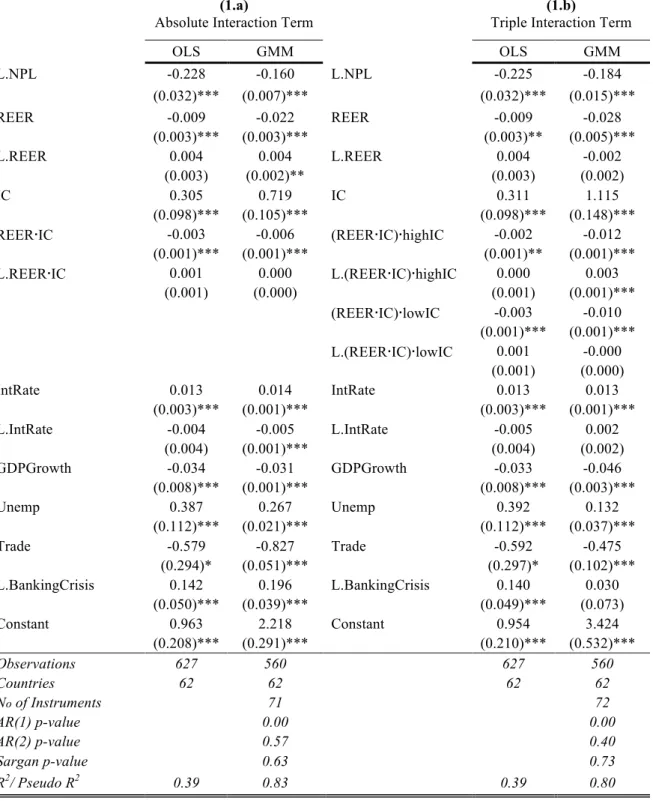
1) Results for Real Effective Exchange Rate
Table 1 displays results obtained from model (1.a) and (1.b). It reveals that real effective exchange rate depreciations in fact lead to an increase of NPLs: In model (1.a), both the coefficient of REER as well as the coefficient of the contemporaneous interaction term are highly statistically significant and carry a negative sign.
The results indicate the following: For very low levels of international claims, currency depreciations and subsequent gains in international competitiveness tend to decrease NPLs ratios. Once the level of international claims increases, exchange rate depreciations indicate a significant negative balance sheet effect, as the costs of servicing foreign currency debt
16 The interpretation of the marginal effects takes the logarithmic structure of the respective variables into
account. Furthermore, Table 1 and 2 represent the model expressed in first differences. In order to interpret the model as the first difference of NPLs, subtracting 𝑁𝑃𝐿$,&,+ on both sides yields the same estimation results where (𝛽+− 1) describes the coefficient of lagged first differenced NPL values.
Ensuing equation (1.a’), the negative balance sheet effect must hold the following condition: −[\ []> 𝐼𝐶
. From
equation (2.a’) follows that uncertainty towards exchange rates drives NPLs when −[\
accrete.18 More specifically, a currency depreciation of one percent contributes to a 1.1% increase in NPLs at the mean level of international claims. At the maximum level of international claims in the sample, the effect is even higher and constitutes an increase in NPLs of 3.2%. On the contrary, when considering the sample minimum of international claims, a depreciation of one percent leads to a 1.1% decrease in NPLs.
Disentangling the effect for countries with high and low international claim levels gives more detail about the distribution of the effect. In both cases, very low levels of international claims translate into a decreasing NPLs ratio following a depreciation of the domestic currency. Hence, in countries with low levels of international claims, gains in international competitiveness outweigh the increased debt servicing cost. Above the respective threshold values, however, negative balance sheet effects clearly dominate and imply an increase of the NPLs ratio following domestic currency depreciations. The marginal effect is stronger for countries with high international claims as compared to countries with lower levels of international claims. For the case of Iceland, for example, with an average international claims ratio as high as 5.0%19, a 1% exchange rate depreciation translates into an increase in non-performing loans of 4.7%, following the estimates.
The findings support the notion of two coexistent opposing channels. Yet, for relevant levels of international claims relative to GDP, negative balance sheet effects clearly dominate and lead to sharp increases in NPLs ratios following an exchange rate depreciation of the domestic currency. The overall impact, i.e. the sum of the lagged and the contemporaneous coefficient also indicates that negative balance sheet effects outsize losses in competitiveness in an intertemporal perspective.
18 The threshold-levels are at 0.026% of international claims relative to GDP for model (1.a), 0.097% for model
(1.b) in a context of high foreign currency debt, and 0.061% for model (1.b) in a context of low foreign currency debt.
Table 1 Determinants of NPLs - Real Effective Exchange Rate
(1.a)
Absolute Interaction Term
(1.b)
Triple Interaction Term
OLS GMM OLS GMM
L.NPL -0.228 -0.160 L.NPL -0.225 -0.184
(0.032)*** (0.007)*** (0.032)*** (0.015)***
REER -0.009 -0.022 REER -0.009 -0.028
(0.003)*** (0.003)*** (0.003)** (0.005)***
L.REER 0.004 0.004 L.REER 0.004 -0.002
(0.003) (0.002)** (0.003) (0.002)
IC 0.305 0.719 IC 0.311 1.115
(0.098)*** (0.105)*** (0.098)*** (0.148)*** REER∙IC -0.003 -0.006 (REER∙IC)∙highIC -0.002 -0.012
(0.001)*** (0.001)*** (0.001)** (0.001)*** L.REER∙IC 0.001 0.000 L.(REER∙IC)∙highIC 0.000 0.003
(0.001) (0.000) (0.001) (0.001)***
(REER∙IC)∙lowIC -0.003 -0.010 (0.001)*** (0.001)*** L.(REER∙IC)∙lowIC 0.001 -0.000
(0.001) (0.000)
IntRate 0.013 0.014 IntRate 0.013 0.013
(0.003)*** (0.001)*** (0.003)*** (0.001)***
L.IntRate -0.004 -0.005 L.IntRate -0.005 0.002
(0.004) (0.001)*** (0.004) (0.002)
GDPGrowth -0.034 -0.031 GDPGrowth -0.033 -0.046
(0.008)*** (0.001)*** (0.008)*** (0.003)***
Unemp 0.387 0.267 Unemp 0.392 0.132
(0.112)*** (0.021)*** (0.112)*** (0.037)***
Trade -0.579 -0.827 Trade -0.592 -0.475
(0.294)* (0.051)*** (0.297)* (0.102)*** L.BankingCrisis 0.142 0.196 L.BankingCrisis 0.140 0.030
(0.050)*** (0.039)*** (0.049)*** (0.073)
Constant 0.963 2.218 Constant 0.954 3.424
(0.208)*** (0.291)*** (0.210)*** (0.532)***
Observations 627 560 627 560
Countries 62 62 62 62
No of Instruments 71 72
AR(1) p-value 0.00 0.00
AR(2) p-value 0.57 0.40
Sargan p-value 0.63 0.73
R2/ Pseudo R2 0.39 0.83 0.39 0.80
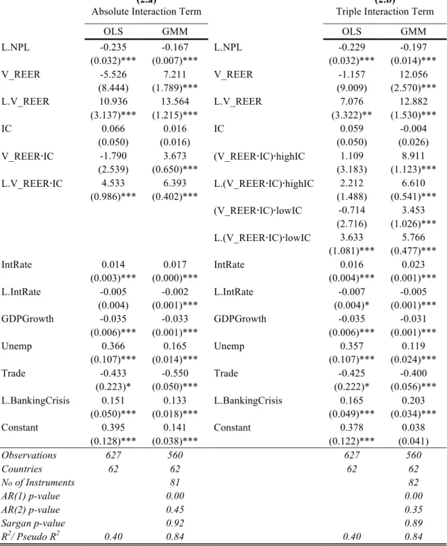
2) Results for Real Effective Exchange Rate Volatility
Table 2 depicts the estimation results based on the models (2.a) and (2.b), employing real effective exchange rate volatility.20 Exchange rate volatility turns out to be highly statistically significant in all specifications and it shows considerable impact on NPLs. According to the estimates for (2.a), a 10 percent change in exchange rate volatility leads to an increase in NPLs of 6.7% at the sample mean level of international claims. The slope of the estimated marginal effect suggests that NPLs react sensibly to volatility in scenarios of high international claims. Volatility in previous periods has an even stronger impact on contemporaneous NPLs.
Looking at the parameters in the right-hand panel allows for a more detailed interpretation: When compared to countries with low international claims, unforeseen exchange rate movements generate considerably more concern towards credit quality in countries with high international claims. The slope of the estimated marginal impact as a function of international claims is roughly four times higher. Therefore, the findings suggest that the more IC a country has the more it is affected by exchange rate volatility.
The results strongly confirm the hypothesis that unforeseen real exchange rate shocks strongly affect NPLs ratios predominantly but not exclusively in countries with high foreign debt levels. However, it must be noted that exchange rate volatility can lead to a reduction of NPLs ratios in scenarios with extremely low international claim levels. In such cases, an alternative interpretation arises: When international claims relative to GDP are low, holders of foreign currency liabilities are more likely to be sufficiently hedged against exchange rate movements. In fact, exchange rate volatility may increase exports and thus openness to
Table 2 Determinants of NPLs - Real Effective Exchange Rate Volatility
(2.a)
Absolute Interaction Term
(2.b)
Triple Interaction Term
OLS GMM OLS GMM
L.NPL -0.235 -0.167 L.NPL -0.229 -0.197
(0.032)*** (0.007)*** (0.032)*** (0.014)***
V_REER -5.526 7.211 V_REER -1.157 12.056
(8.444) (1.789)*** (9.009) (2.570)***
L.V_REER 10.936 13.564 L.V_REER 7.076 12.882
(3.137)*** (1.215)*** (3.322)** (1.530)***
IC 0.066 0.016 IC 0.059 -0.004
(0.050) (0.016) (0.050) (0.026)
V_REER∙IC -1.790 3.673 (V_REER∙IC)∙highIC 1.109 8.911
(2.539) (0.650)*** (3.183) (1.123)***
L.V_REER∙IC 4.533 6.393 L.(V_REER∙IC)∙highIC 2.212 6.610
(0.986)*** (0.402)*** (1.488) (0.541)***
(V_REER∙IC)∙lowIC -0.714 3.453 (2.716) (1.026)*** L.(V_REER∙IC)∙lowIC 3.633 5.766
(1.081)*** (0.477)***
IntRate 0.014 0.017 IntRate 0.016 0.023
(0.003)*** (0.000)*** (0.004)*** (0.001)***
L.IntRate -0.005 -0.002 L.IntRate -0.007 -0.005
(0.004) (0.001)*** (0.004)* (0.001)***
GDPGrowth -0.035 -0.033 GDPGrowth -0.035 -0.031
(0.006)*** (0.001)*** (0.006)*** (0.001)***
Unemp 0.366 0.165 Unemp 0.357 0.119
(0.107)*** (0.014)*** (0.107)*** (0.024)***
Trade -0.433 -0.550 Trade -0.425 -0.400
(0.223)* (0.050)*** (0.222)* (0.056)***
L.BankingCrisis 0.151 0.133 L.BankingCrisis 0.165 0.203 (0.050)*** (0.018)*** (0.049)*** (0.034)***
Constant 0.395 0.141 Constant 0.378 0.038
(0.128)*** (0.038)*** (0.122)*** (0.041)
Observations 627 560 627 560
Countries 62 62 62 62
No of Instruments 81 82
AR(1) p-value 0.00 0.00
AR(2) p-value 0.45 0.35
Sargan p-value 0.92 0.89
R2/ Pseudo R2 0.40 0.84 0.40 0.84
The dependent variable is the first difference of NPLs in natural logarithm. Standard errors in parentheses.
international trade, leading to more favorable financial positions of borrowers and to efficiency gains through spillover effects to the economy (De Grauwe, 1988).21
In accordance to the existing literature, in all models (both for the ones with the real effective exchange rate as well as the real effective exchange rate volatility) real GDP growth leads to a decline in NPLs. According to the estimates, a GDP growth of 1 percent translates into a reduction of NPLs between 3.1% and 4.6% at a significance level of 1%. This confirms that NPLs are countercyclical, meaning that the NPLs ratio rises in recessions and decreases in business cycle upturns. The magnitude of the coefficients implies that the economic climate has a strong negative impact on the financial stability. High unemployment rates as well as high lending interest rates are driving forces of NPLs. These findings are highly significant and robust across all models. The coefficients of the trade variable show the expected negative sign and statistical significance at a 1% level throughout all estimations. The results furthermore provide evidence that the occurrence of a banking crisis in previous periods is an important driver of NPLs.
4.1 Robustness
High foreign currency denoted liabilities are understood to be a financial-economic weakness of emerging markets.22 Looking at the Mexican tequila crisis (1994), the Russian ruble crisis (1998) and the East Asian crisis in the end of the 20th century, it is evident that high foreign currency debt levels have magnified the severity of the crises (Eichengreen and Hausmann, 1999). Therefore, as yet another means to evaluate the robustness of the findings, a different sample was taken into account: The reduced sample consists of 21 emerging markets,
21 De Grauwe (1988) established a theoretical model on the relationship of exports and exchange rate volatility.
In fact, many empirical approaches, such as Kasman and Kasman (2005) and Doyle (2001) build evidence for such a relation.
22
following J.P. Morgan’s Emerging Market Bond Index categorization.23 The time period covered remains the same (2000-2014). Given the reduced sample and to avoid problems of overidentifying restrictions, the identification strategy differs slightly: I introduce an index of financial market development, obtained from the World Economic Forum’s Global Competitive Index Historical Dataset, as a control variable. Moreover, I do not longer segregate into high or low foreign currency debt holding economies so that only the absolute interaction term is applied. The unemployment variable is dropped from the regression. At this point, it is important to mention that reducing a sample size must be always treated with caution, because it can lead to a loss of estimation efficiency and the explanatory power of the model may dilute.
Table A.7 in the Appendix presents the results of the emerging markets estimation. The results underline the robustness of my previous findings. According to the coefficients of the
REER model (3.a), both the contemporaneous value of REER as well as interacted with international claims are statistically significant and carry a negative sign. This reinforces the previous results from the complete sample, as the negative balance sheet effect dominates again. Furthermore, the magnitude of the estimated coefficients proves that the marginal effect of exchange rate movements on NPLs is higher for emerging markets compared to the full sample. Given the tremendous increase of unhedged foreign currency debt in emerging markets,24 exchange rate movements have to be understood as a considerable threat for the financial stability in those countries. In the case of the exchange rate volatility (3.b), the lagged values show statistical significance and a positive sign. This implies that the unexpected shocks in previous periods have to be seen as an important determinant of NPLs and consequently a serious concern for the financial stability of emerging markets.
23
List of countries in Table A.6 in the Appendix.
4.2 Limitations and Future Research
Even though I handled the data as well as the methodological approach with great care, the analysis may be subject to a number of caveats. First, as indicated above, data on NPLs is likely to not be uniformly reported across all countries in the sample. This raises justified concerns regarding the external validity of the results. Second, international claims are only a proxy for foreign currency lending in the model. It is plausible that more accurate data would significantly improve the interpretational power of the results. Lastly, a meaningful draw-back of the approach lays within the measurement of exchange rate volatility: The standard deviation of first differences, despite controlling for trends, is an outlier-insensitive measure and may thus fail to capture peak-values of the exchange rate. However, such extrema may contain relevant information on the state of the economy that are neglected in this measure (Serenis and Tsounis, 2012).
There are interesting avenues for future research regarding the measurement of volatility. An extension to the measure used in this paper is the long-run volatility. This measure can be derived by the standard deviation of monthly logarithmic differences in exchange rates calculated over the preceding five years. One would expect, that this measure of volatility is larger than the average short-run volatility over the same years. Once there are more data points on NPLs available, such an approach may improve upon existing research.
Furthermore, a GARCH approach can be applied in order to forecast volatility based on past values of exchange rate. This has the benefit to capture unforeseen movements by calculating the deviations between actual and predicted exchange rate values.
5 Conclusion
the quality of bank assets, meaning that higher debt servicing costs (negative balance sheet effect) dominate financial gains from higher exports in international markets (trade effect). This implies that in countries with currency mismatches, a depreciation of the local currency tends to increase NPLs. In the recent global economic situation, this exchange rate risk materialized in countries with currency mismatches in their accounts: Looking at the European Union, for example, the depreciation of local currencies in Central, Eastern and Southeast Europe against the Swiss Franc has severely affected default rates in a negative way. This is particularly true for countries like Poland, Hungary and Croatia, which hold a high amount of Swiss Franc denominated debt. Another example is Iceland during the financial crisis: Between 2006 and 2010, The Icelandic Krona depreciated tremendously both against the US Dollar as well as the Euro. At the same time, NPLs in the Nordic country jumped up by 17.5%.25
Furthermore, the findings indicate that exchange rate volatility has a strong and positive impact on NPLs, suggesting that bank asset quality reacts sensibly to unforeseen exchange rate shocks. In fact, recent economic events prove the importance of exchange rate volatility for the financial-economic stability of a country: Looking at the Argentinian Peso, for example, 2014 brought enormous exchange rate swings due to black market activity and the nomination of a new president of the federal bank. Non-performing loans, as a result, exploded after a period of low default rates following the crisis. Another example is the sudden removal of the Swiss Franc – Euro peg in 2015. Several countries experienced a tremendous increase of debt servicing costs inducing significant problems to repay foreign currency loans. The Hungarian government, as an example, was forced to take extraordinary steps in order to prevent massive loan defaults, as it allowed borrowers to convert expensive Swiss Franc - denominated debt into domestic Forint liabilities.
Summing it up, the findings suggest that countries with currency mismatches are exposed to considerable credit risk as a result of exchange rate movements and exchange rate uncertainty. The policy implication following these conclusions are clear: Countries with high foreign currency claims that are not sufficiently offset by foreign currency assets should pay increased attention to hedge national currencies and consider to follow a fixed-rate regime. The results of this paper are a contribution to existing macro-prudential stress testing: Including exchange rate movements as well as exchange rate volatility increases the accuracy of this scenario testing and draws a more realistic and reliable picture of the state of credit conditions in countries with foreign currency liabilities.
6 References
Aghion, Philippe, Bacchetta, Philippe, Ranciere, Romain, and Rogoff, Kenneth. 2009. "Exchange rate volatility and productivity growth: The role of financial development." Journal of Monetary
Economics 56(4): 494-513.
Arellano, Manuel, and Stephen Bond. 1991. "Some tests of specification for panel data: Monte Carlo evidence and an application to employment equations." The Review of Economic Studies 58(2): 277-297.
Basel Committee on Banking Supervision. 2006."Basel II: International Convergence of Capital Measurement and Capital Standards: A Revised Framework - Comprehensive Version."
Beck, Roland, Petr Jakubik, and Anamaria Piloiu. 2015. "Key determinants of non-performing loans: new evidence from a global sample." Open Economies Review 26(3): 525-550.
Bond, Stephen R., Anke Hoeffler, and Jonathan RW Temple. 2001. "GMM estimation of empirical growth models." Economics Papers 21.
Bordo, Michael D., and Christopher M. Meissner. 2006. "The role of foreign currency debt in financial crises: 1880–1913 versus 1972–1997." Journal of Banking & Finance 30(12): 3299-3329.
Chui, Michael KF, Ingo Fender, and Vladyslav Sushko. 2014. "Risks related to EME corporate balance sheets: the role of leverage and currency mismatch." BIS Quarterly Review September.
Clark, Peter, Natalia Tamirisa, Shang-Jin Wei, Azim Sadikov, and Li Zeng. 2004. "Exchange rate volatility and trade flows-some new evidence." IMF Occasional Paper 235.
De Grauwe, Paul. 1988. "Exchange rate variability and the slowdown in growth of international trade." IMF Economic Review 35: 63-84.
Dickey, David A., and Wayne A. Fuller. 1981. "Likelihood ratio statistics for autoregressive time series with a unit root." Econometrica: Journal of the Econometric Society: 1057-1072.
Doyle, Eleanor. 2001. "Exchange rate volatility and Irish-UK trade, 1979-1992." Applied Economics 33(2): 249-265.
Espinoza, Raphael A., and Ananthakrishnan Prasad. 2010. "Nonperforming loans in the GCC banking system and their macroeconomic effects." IMF Working Papers: 1-24.
European Central Bank. 2016. "Financial Stability Review May 2016. " Accessed November 10th, 2016. https://www.ecb.europa.eu/pub/fsr/html/index.en.html.
Glen, Jack, and Camilo Mondragón-Vélez. 2011. "Business cycle effects on commercial bank loan portfolio performance in developing economies." Review of Development Finance 1 (2): 150-165.
Hausmann, Ricardo, Ugo Panizza, and Ernesto Stein. 2001. "Why do countries float the way they float?." Journal of Development Economics 66(2): 387-414.
Im, Kyung So, M. Hashem Pesaran, and Yongcheol Shin. 2003. "Testing for unit roots in heterogeneous panels." Journal of Econometrics 115(1): 53-74.
IMF. 2006. "The Financial Soundness Indicators Compilation Guide of March 2006." Accessed November 10th, 2016. https://www.imf.org/external/pubs/ft/fsi/guide/2006/
Jesus, Saurina, and Jimenez Gabriel. 2006. "Credit cycles, credit risk, and prudential regulation." International Journal of Central Banking 2: 65-98.
Kasman, Adnan, and Saadet Kasman. 2005. "Exchange rate uncertainty in Turkey and its impact on export volume." METU Studies in Development 32(1): 41-58.
Krueger, Russell. 2002. "International standards for impairment and provisions and their implications for financial soundness indicators (FSIs)." Manuscript, International Monetary Fund.
Lane, Philip R., and Jay C. Shambaugh. 2010, "Financial exchange rates and international currency exposures." The American Economic Review 100(1): 518-540.
Louzis, Dimitrios P., Angelos T. Vouldis, and Vasilios L. Metaxas. 2012. "Macroeconomic and bank-specific determinants of non-performing loans in Greece: A comparative study of mortgage, business and consumer loan portfolios." Journal of Banking & Finance 36(4): 1012-1027.
Nkusu Mwanza. 2011. "Nonperforming loans and macrofinancial vulnerabilities in advanced economies." IMF Working Paper 11/161.
Pesola, Jarmo. 2005."Banking fragility and distress: An econometric study of macroeconomic determinants." Bank of Finland Research Discussion Paper 13.
Podpiera, Jiri, and Inci Ötker-Robe. 2010. "The fundamental determinants of credit default risk for European large complex financial institutions." International Monetary Fund Working Paper 10/153.
Rodriguez, Francisco, and Dani Rodrik. 2001. "Trade policy and economic growth: a skeptic's guide to the cross-national evidence." NBER Macroeconomics Annual 2000 15: 261-338. MIT Press.
Roodman, David. 2009. "A note on the theme of too many instruments. " Oxford Bulletin of
Economics and Statistics 71(1): 135-158.
Salas, Vicente, and Jesus Saurina. 2002. "Credit risk in two institutional regimes: Spanish commercial and savings banks." Journal of Financial Services Research 22(3): 203-224.
Serenis, Dimitrios, and Nicholas Tsounis. 2012. "A new approach for measuring volatility of the exchange rate." Procedia Economics and Finance 1: 374-382.
Valencia, Fabian, and Luc Laeven. 2012. "Systemic banking crises database: An update."
International Monetary Fund Working Paper 12/163.