Rui Jorge Freitas Rodrigues Guimarães
Development of a signal processing tool for
the post-processing of structural dynamics
results obtained through the application of
the finite element method.
Tese de Mestrado
Mestrado Integrado em Engenharia Mecânica
Trabalho efetuado sob a orientação do
Doutor José Felipe Bizarro de Meireles
Co-orientador
Doutor Paulo Jorge da Rocha Soares
Antunes
iii
pessoas, que, através de apoio científico ou incentivos pessoais, me levaram a concretizar este projecto, e sem os quais não o teria conseguido.
Aos meus orientadores, Doutor José Felipe Bizarro de Meireles e Doutor Paulo Jorge da Rocha Soares Antunes, dirijo uma palavra de agradecimento, por todo o tempo que disponibilizaram a este projecto e pela forma como me souberam orientar.
Ao Doutor Gustavo Rodrigues Dias e Doutor Júlio César Machado Viana, que me permitiram usufruir, por diversos momentos, dos recursos da empresa em prol da realização deste trabalho, e todos os colaboradores da Critical Materials S.A. que de alguma forma me auxiliaram na realização deste trabalho, envio também uma palavra de agradecimento.
Gostaria de agradecer à minha família e amigos que nunca deixaram de acreditar no meu trabalho. Por fim, uma especial palavra de apreço e agradecimento a quem teve a generosidade (e muitas vezes paciência) de ser o meu maior suporte, Maria João.
v
problems is resulting in a growing interaction with auxiliary tools, such as signal processing tools, able to extend the FEM efficiency. The incorporation of such tools in finite element analysis (FEA) software is a reality. Therefore, this work aimed the development of a signal processing tool for the post-processing of structural dynamics results obtained through the application of the finite element method.
The tool was developed as a plug-in, in order to be fully embedded into Abaqus®
Non-linear FEA platform, and provides those signal processing algorithm, considered as being the most relevants in the structural dynamic analysis field.
In order to demonstrate the potentialities of the developed tool three case-studies were developed where is proved the advantages of such tool when applied to structural dynamics analysis problems.
vii
relacionados com a dinâmica estrutural tem resultado numa crescente interacção com ferramentas auxiliares, tais como ferramentas para o processamento de sinal, capazes de aumentar a eficiência do próprio FEM. A inclusão destas ferramentas em software’s dirigidos à análise de elementos finitos (FEA) é uma realidade. Assim sendo, pretendeu-se, com este trabalho, o desenvolvimento de uma ferramenta para pós-processamento de resultados obtidos em análise de dinâmica estrutural recorrendo ao método dos elementos finitos.
A ferramenta foi desenvolvida sob a forma de plug-in, de modo a ser embebida na plataform Abaqus® Non-linear FEA, e comtempla os algoritmos de processamento de sinal considerados mais relevantes no domínio da dinâmica estrutural.
Com o objetivo de demonstrar as potencialidades da ferramenta desenvolvida foram conduzidos três casos de estudo onde se prova o interesse da ferramenta na aplicação a problemas de dinâmica estrutural.
ix
Abstract v
Resumo vii
Contents ix
List of figures xi
List of tables xvii
List of symbols xix
1 Introduction 1
1.1 Motivation 2
1.2 Outline of the thesis 3
2 State of the art 5
2.1 Dynamic analysis 5
2.1.1 Single degree of freedom 6
2.1.2 Multi degree of freedom system 23
2.2 Signal processing 25
2.2.1 Signal acquisition 26
2.2.2 Signal types 28
2.3 Theoretical introduction to the problem 31
2.3.1 Signal processing of discrete signals 32
2.3.2 Structural dynamics analysis 35
2.3.3 Finite element analysis 49
3 Signal Processing for Abaqus® 53
3.1 General view 54 3.2 Modules 57 3.2.1 Transformations 58 3.2.2 Statistical operations 62 3.2.3 Signal operations 66 3.2.4 Advanced operations 68
4 Case-studies 71
4.1 Oberst beam method for material characterisation 71
4.1.1 Introduction 71
4.1.2 Objective 72
4.1.3 Definitions and acronyms 72
4.1.4 Contextualization 72
4.1.5 Procedure 73
4.1.6 FE modelling 73
4.1.7 Results 76
4.1.8 Results discussion 80
4.2 Study about Lamb waves’ sensitivity in the damage identification 81
4.2.1 Introduction 81
4.2.2 Objective 82
4.2.3 Definitions and acronyms 83
4.2.4 Contextualization 83 4.2.5 FE modelling 84 4.2.6 Results discussion 87 4.3 A PRODDIA® deployment 93 4.3.1 Introduction 93 4.3.2 Objective 93
4.3.3 Definitions and acronyms 94
4.3.4 Contextualization 94
4.3.5 FE modelling 95
4.3.6 Mesh convergence studies 99
4.3.7 Sensor Positioning 104
4.3.8 Results discussion 105
5 Conclusions and future work 107
Bibliography 109
Annex A Transforms methods 113
Annex B SPA requirements 117
xi
Figure 2.2 Damped SDOF system disturbed by a force, 𝑓(𝑡). 6 Figure 2.3 Damped SDOF system disturbed by a base motion, 𝑥𝑏(𝑡). 7 Figure 2.4 Free vibration of an undercritically-damped SDOF system. (Source: Braun et al.
(2002)) 9
Figure 2.5 Vector diagram of forces. 11
Figure 2.6 FRF magnitude and phase angle varying with the damping ratio, for a given
undercritically-damped SDOF system. 12
Figure 2.7 Arbitrary periodic loading. (Source: Clough and Penzien (1993)) 12
Figure 2.8 Arbitrary impulsive loading. 13
Figure 2.9 Impulse response function for an arbitrary undercritically-damped SDOF system. 14 Figure 2.10 Derivation of the Duhamel's integral. 15 Figure 2.11 3-D plots representing the transfer function magnitude, 𝐻 (left), and phase angle, 𝜃
(right), in the 𝑠-plane, highlighting the frequency response function, represented by
the dashed line. 17
Figure 2.12 FRF amplitude, highlighting the resonance, for an arbitrary undercritically-damped SDOF system. (Source: Clough and Penzien (1993)) 19 Figure 2.13 Schematic representation of Convolution, Cross-correlation and Autocorrelation
operations. (Source: wikipedia.org) 21
Figure 2.14 Damped MDOF system. 23
Figure 2.15 Exemplificative response of a MDOF system to a transient loading in the time domain (left) – acceleration – and, the respective frequency par, in the Fourier domain (right)
– accelerance. 25
Figure 2.16 Typical examples of signals: (A) Continuous (analogue) signal; (B) Discrete signal (digital), sampled at every ∆ seconds. 27 Figure 2.17 Schematic diagram of a general data acquisition system. A/D, analogue-to-digital. 28 Figure 2.18 Signal types. (Source: Randall (1987)) 28 Figure 2.19 Sinusoidal signal with a period 𝑇 [s]. 29 Figure 2.20 Hum noise signal. (Source: Shin and Hammond (2008)) 29
Figure 2.21 White noise signal. 30 Figure 2.22 Typical example of transient signals. 30 Figure 2.23 Typical example of non-stationary signals. (Source: Shin and Hammond (2008)) 31 Figure 2.24 Magnitude spectrum of a FRF highlighting the resonance peaks, and the half-power
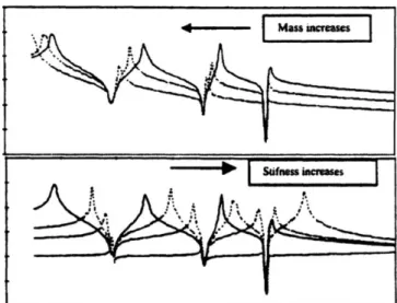
(-3 dB) points, for each mode. (Source: Brüel & Kjær (1999)) 35 Figure 2.25 Impact of modifications on the structural dynamic behaviour of a cantilever beam.
(Source: Silva and Maia (1999)) 36
Figure 2.26 Tacoma Narrows Bridge roadway, vibrating (left) and finally collapsing (right), due to excitation forces produced by wind (traveling at 64𝑘𝑚ℎ). (Source: wikipedia.org) 37 Figure 2.27 Frequency response of an MDOF (A) system, and the highlighting of the respective
SDOF modal contributions (B) – Note: The plots are zooming the first three modes in range). (Source: Agilent Technologies (2000)) 39 Figure 2.28 System descriptors, time and frequency domain. (Source: Bilošová (2011)) 41 Figure 2.29 Basic experimental rig for modal testing. (Source: Brüel & Kjær (1999)) 42 Figure 2.30 “Free” conditions. (Source: Agilent Technologies (2000)) 43 Figure 2.31 Grounded condition. (Source: SEM Modal Analysis Technical Division (2011)) 43 Figure 2.32 Complex mechanical structures in operation: (A) Offshore petroleum platform; (B)
Wind turbine. (Source: Barakah Offshore Petroleum (2014) and Vestas Wind Systems
A/S (2014)) 43
Figure 2.33 Civil structures under monitoring: (A) Bridge; (B) Stadium suspended roof. (Source: SC Solutions (2013) and Magalhães et al. (2006)) 44 Figure 2.34 Shake excitation: (A) shaker mass influence; (B) typical experimental setups.
(Source: Agilent Technologies (2000)) 45 Figure 2.35 Impact hammer excitation: (A) Instrumented impact hammer; (B) typical curves of
excitations with different “tips”. (Source: National Instruments Corporation (2014)
and Agilent Technologies (2000)) 45
Figure 2.36 Influence of mass loading on measured response. (Source: Agilent Technologies
(2000)) 46
Figure 2.37 2-D and 3-D representation of a MAC matrix values, for the modes shape correlation.
(Source: Braun et al. (2002)) 47
Figure 2.38 Several sets of (x, y) points, with the correlation coefficient of x and y for each set. Note that the correlation reflects the non-linearity and direction of a linear relationship (top row), but not the slope of that relationship (middle), nor many aspects of
nonlinear relationships (bottom). 49
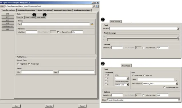
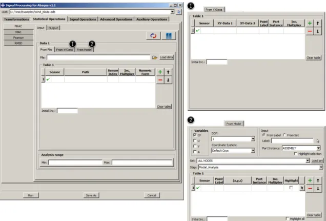
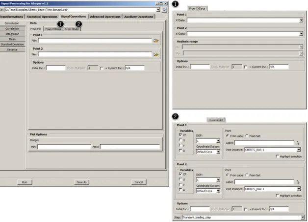
From XYData and From Model tabs. 58 Figure 3.6 Defining input variables for FFT procedure. 59 Figure 3.7 FFT resultant spectrums: Magnitude and Phase angle 60 Figure 3.8 Input and output definition to obtain the FRF response (compliance). 60 Figure 3.9 Compliance resultant spectrums, Magnitude and Phase angle. 61 Figure 3.10 General view of Statistical Operations category, presenting the typical aspect of From
File, From XYData and From Model tabs. 62 Figure 3.11 Inputs definition for both “source data”, Data 1 and Data 2, to run MAC procedure.
63 Figure 3.12 MAC correlation output matrix result. 64 Figure 3.13 Inputs definition to obtain the FRAC correlation between two systems responses
obtained from experimental and analytical tests. 64
Figure 3.14 FRAC correlation output. 65
Figure 3.15 General view of Signal Operations category, presenting the typical aspect of From File, From XYData and From Model tabs. 66
Figure 3.16 Acceleration signal. 67
Figure 3.17 Defining inputs to perform the correlation. 67 Figure 3.18 Autocorrelation of signal presented in Figure 3.16. 68 Figure 3.19 General view of Advanced Operations category, presenting the typical aspect of From File, From XYData and From Model tabs. 68 Figure 3.20 Selection of the magnitude part resultant for the FFT procedure in section 3.2.1.1. 69 Figure 3.21 Results obtained from the extraction of modal damping (%) values from a compliance
response (magnitude part). 70
Figure 4.1 Experimental setup. Cantilever Oberst Beam. (Source: Antunes, et al. (2009)) 73 Figure 4.2 Oberst beam general dimensions. 74
Figure 4.3 Oberst beam FE model. 75
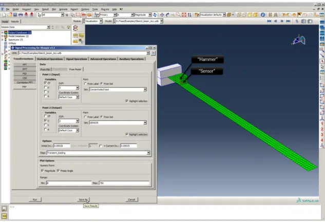
Figure 4.5 SPA procedure to obtain the compliance spectrums (see example in section 3.2.1.1): input (“Hammer”) – Concentrated load node set; output (“Sensor”) – Sensor node
set. 77
Figure 4.6 Transient signals in time domain: Input (“hammer”) and output (“sensor”). 78 Figure 4.7 Highlight of three identified modes from the resultant compliance magnitude part
spectrum analysis (inputs in Figure 4.5). 78 Figure 4.8 Compliance spectrum – LabView®. (Source: Antunes et al. (2009)) 79
Figure 4.9 Fraction of critical damping (𝜉) with frequency– LabView®. (Source: Antunes et al.
(2009)) 79
Figure 4.10 Fraction of critical damping [%]: experimental Vs analytical results. 80 Figure 4.10 Phase velocity dispersion curves for Lamb waves in steel plate, showing shapes of
fundamental modes. (Source: Braun et al. (2002)) 82
Figure 4.12 Test scenario. 83
Figure 4.13 Test scenario general dimensions. 84 Figure 4.14 Mesh details, highlighting the “damage” area (only applicable for the damage
model). 86
Figure 4.15 15 kHz (sine wave) tone burst 3.5 cycles Hann windowed pulse 87 Figure 4.16 Electrical potential boundary conditions. 87 Figure 4.17 FFT (magnitude part) spectrum obtained from the transformed time domain velocity
from a central point of the PZT top layer, obtained using SPA FFT module. 88 Figure 4.18 Lamb wave propagation state (elapsed time 0.0002s) in the CFRP plate. 89 Figure 4.19 Wavelet propagation, from PZT point to “Sensor” point. Boundary reflection effect is
also emphasised. 89
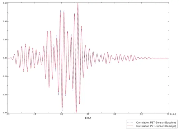
Figure 4.20 Baseline and damage models in a given, step time frame. 90 Figure 4.21 Comparison of signals (normal to surface velocity): baseline Vs damage models. 90 Figure 4.22 Picking point to extract data using the SPA Correlation module. 91 Figure 4.23 Comparison of cross-correlated signals (normal to surface velocity): baseline Vs
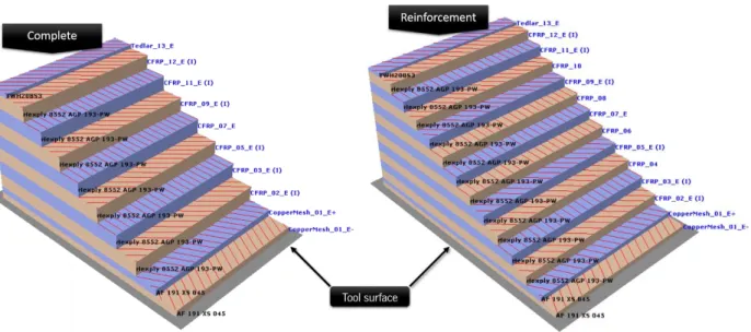
damage models, obtained using the SPA Correlation module. 92 Figure 4.24 Experimental setup to test CSHM1 structure. 94 Figure 4.25 CSHM1 component general dimensions and composite plies layup scheme. 95 Figure 4.26 CSHM1 composite plies stacking order. 96 Figure 4.27 CSHM1 final layup: complete, reinforcement, and overlap areas. 96 Figure 4.28 Example of complete and reinforcement layups (discretised in element). 97
Figure 4.31 Meshes – (i) Mesh A: used to define Mesh A-S4R and Mesh A-S8R; (ii) Mesh B –
used to define Mesh B-S8R. 100
Figure 4.32 Points (“sensors”) locations from where modal displacement, U2, was extracted. 101 Figure 4.33 Inputs selection to run the SPA’s MAC analysis (Mesh S4R Vs Mesh B-S8R). 101 Figure 4.34 SPA’s MAC analysis output results (Mesh S4R Vs Mesh B-S8R). 102 Figure 4.35 MAC output matrix results: (i) Mesh A-S4R Vs Mesh B-S8R; (ii) Mesh A-S8R Vs Mesh
B-S8R. 103
Figure 4.36 CSHM1first four eigenmodes (study “1st moment”). 104
Figure 4.37 CSHM1resultant Sensor Positioning field (study “1st moment”). Locations for four
xvii
Table 2.2 Physical quantities possible to be measured from a system. 40
Table 3.1 Requirement table template. 53
Table 3.2 Modules domains. 56
Table 4.1 Initial material properties. 74
Table 4.2 Modal damping values: analytical. 78 Table 4.3 Modal damping values: experimental. 80
Table 4.4 Initial material properties. 85
Table 4.5 CSHM1 composite plies layup. 96
Table 4.6 Initial material properties. 97
xviii
xix
𝐴 Generic complex number (magnitude) 𝐴1, 𝐴2 Constants
𝑏0, 𝑏𝑛 Fourier coefficients constants 𝑐 𝑘𝑔𝑠−1 Damping coefficient
[𝑐] 𝑘𝑔𝑠−1 Damping coefficient matrix 𝑒 Exponential
𝐸 𝑁𝑚−2 Young’s modulus 𝑓 𝐻𝑧 Natural cyclic frequency 𝑓(𝑡) 𝑁 Applied loading in time domain
𝐹(𝑖𝜔) Load vector in frequency domain (Fourier transform) 𝐹(𝑠) Load vector in the Laplace domain
𝑓𝐼, 𝑓𝐷, 𝑓𝑆 𝑁 Inertial, damping, and spring forces, respectively 𝑓𝐼, 𝑓𝐷, 𝑓𝑆 𝑁 Inertial, damping, and spring forces, respectively
𝐺 𝑁𝑚−2 Shear modulus
𝑔(𝑡) Generic function in time domain
ℎ(𝑡) Impulse response function in time domain 𝐻(𝑖𝜔) Frequency response function in frequency
𝑖 √−1 Imaginary number 𝑗 Arbitrary coordinate 𝐼0 𝑁𝑠 Impulse-momentum
𝑘 𝑁𝑚−1 Spring stiffness constants, frequency domain index, arbitrary coordinate
[𝑘] 𝑁𝑚−1 Spring stiffness constants matrix 𝑚 𝑘𝑔 Mass, time index
[𝑚] 𝑘𝑔 Mass matrix
𝑛 Integer, constant, time domain index
𝑁 Number of time increments, number of degree of freedom, number of resonance peaks
𝑅𝑥𝑦(𝜏) Cross-correlation function
𝑟 Mode number, Pearson’s correlation coefficient 𝑠 Laplace constant
𝑆𝑋𝑋(𝑖𝜔) 𝑔2𝐻𝑧−1 Power spectral density function 𝑆𝑋𝑌(𝑖𝜔) 𝑔2𝐻𝑧−1 Cross-spectral density function
𝑡, 𝑡0 𝑠 Time
𝑇, 𝑇𝑝 𝑠 Period of vibration 𝑣0 𝑚𝑠−1 Initial velocity 𝑥0 𝑚 Initial displacement
𝑥(𝑡) 𝑚 Displacement function in time domain, generic time domain signal 𝑥𝑏(𝑡) 𝑚 Base motion function in time domain
𝑥𝑐(𝑡), 𝑥𝑝(𝑡), 𝑚 Particular and complementary solutions, respectively. 𝑦(𝑡) Generic time domain signal
𝛽 Frequency ratio
𝛿(𝑡) Dirac’s delta function in time domain 𝜃 𝑟𝑎𝑑 Angle 𝜆 Eigenvalue 𝜉, 𝜉𝑛,𝜉𝑟 Damping ratios 𝜏 𝑠 Time delay 𝜙 Mass-normalised Eigenvector Φ Modal matrix
𝜓 Eigenvector (mode shape vector) Ψ Mode shapes matrix
𝜌 Vector magnitude
𝜔 𝑟𝑎𝑑𝑠−1 Circular frequency, eigenvalue 𝜔𝑛 𝑟𝑎𝑑𝑠−1 Undamped natural circular frequency 𝜔𝑑 𝑟𝑎𝑑𝑠−1 Damped natural circular frequency
Operators
( )∗ Complex conjugate ( ̇ ) First order derivate ( ̈ ) Second order derivate
| | Vector norm (∗) Convolution
xxiii
API Application programming interface CAD Computer Aid Design
CSD Cross-spectral density DAQ Data acquisition system DOF Degree of freedom DFT Discrete Fourier transform FEA Finite element analysis FE Finite elements FEM Finite element method FFT Fast Fourier transform
FRAC Frequency response assurance criteria FRF Frequency response function
GUI Graphical user interface
IDFT Inverse discrete Fourier transform
IEEE Professional association for the advancement of technology IFFT Inverse fast Fourier transform
IRF Impulse response function MAC Modal assurance criteria MDOF Multiple degree of freedom ODB Output database
PSD Power spectral density RMSD Root mean square deviation SDA Structural dynamic analysis SDOF Single degree of freedom SHM Structural heath monitoring SPA Signal Processing for Abaqus TF Transfer function
1
1
Introduction
Nowadays, Structural Dynamics Analysis (SDA) is largely associated with computational mechanics, which has in the Finite Element Method (FEM) the most significant analysis tool. The application of computational mechanical procedures, such as FEM, to design complex structures, like bridges, cars, planes, satellites, space crafts, dams, tool machines, etc., is considered fundamental in modern engineering fields. FEM enables the access to information from analytical models, which is used to predict the dynamic behaviour of the analysed structure or component. In the SDA field, post-processing operations on dynamic signals are crucial for evaluating, more in detail, particular aspects such as resonance frequencies, punctual accelerations, vibration spectra, etc. In this way, is crucial to have tools that can be used to improve and optimize such signal processing operations, specially, tools embedded in the analysis framework.
As stated by the IEEE Signal Processing Society, in their most recent constitution document (IEEE Signal Processing Society, 2012), “signal processing is the enabling technology for the generation, transformation, extraction, and interpretation of information.”, and for Oppenheim et al. (1998), signal processing is concerned with the representation, transformation, and manipulation of signals and the information they contain.
SDA, in particular, has benefited, and keep collecting profits, from the continuum improvement of the signal processing techniques. These technics are used by dynamicist analysts to improve the FEM capabilities, extending the method beyond the project phase. Examples of such extended application, are given by Viana et al. (2011), Kluska et al. (2012), Epameinondas et al. (2009), in works involving Finite Element (FE) models to assess damage in mechanical structures in the context of Structural Health Monitoring Techniques (SHM).
The continuum increase of computational power together with the enhancement of the theories behind FEM development, led Khennane (2013) to write that FEM will continually increase its capability of recreate more accurate models from real structures, enabling the access to relevant and more precise information about the structural dynamic behaviour of real structures or components. By other side, the complexity of FE models tends to increase. This means that, with
the continuous increase in the complexity of modelled structures, large amounts of data will be available for post-processing operations.
FE analysts, normally, use third-party software to execute dynamic signal processing operations compromising the interactivity with the FE model. Time spent in pre-process data files for posterior upload to external software’s is high and tends to increase the probability of analysis errors, compromising the ability to execute “on-the-fly” operations. Moreover, dedicated numerical computational tools for signal processing are very expensive and, most of the time, are not able to interact, directly, with the FE model.
1.1 Motivation
Current structural dynamics analysis demands quick and reliable solutions for complex problems. Dynamic analysts have been using FEM to solve highly complex dynamic problems. They been comparing experimental and analytical data, using signal processing techniques, in order to predict and compare structural dynamic behaviour. In this field, FEM proves to be a truly effective and reliable method to solve dynamic problems, and for some authors (Clough and Penzien, 1993), has become the standard tool for structural dynamicists. Massive use of FEM led to a huge improvement on the FEM tools, which has in commercial finite-element codes some of the best applications to solve problems related with SDA. Commercial finite-element software became so advanced that even nonlinearity (material or geometrical), contact, structural interaction with fluids, metal forming, crash simulation, and several other problems, can be modelled and solved with extreme efficiency.
The increasing reliability of FEM methods led many experts to relay on finite-element software to aid in the structural design, taking some authors (Khennane, 2013) to affirm that, nowadays, all but simple structural analysis, in structural design are carried out using FEM.
The trend on the analysis of SDA is to include more dynamical insight on current problems, which generates temporal and frequency dependent information of the relevant physical variables. These resultant variables play the most important role on this procedure, since the main aim of the FEM it is to get information from the virtual model and compare/correlate them to the signals acquired from the real structure (Antunes et al., 2012).
Although numerical methods can give reliable solutions for many complex problems, still necessary to use experimental tests to validate many of these analytical solutions (Meireles, 2007). Even so, FEM allows to test methodologies and theories, involving structural dynamic behaviour,
handled, that is usually exported from the original FE software in order to be post-processed by a third-party software. However, to avoid deceiving conclusions or mismatch of experimental Vs analytical data, it is mandatory to guarantee a consistent manipulation of outputted results.
This work intends to design and obtain a signal processing tool able to post-process Finite Element Analysis (FEA) in an embedded form, increasing the efficiency of dynamic analysis in the SDA field. This tool aims to be used by advanced FE analysts that use Abaqus® Non-linear FEA package (from now on, designated simply as Abaqus®), as platform for FEA. A fully embedded solution, capable of performing the most relevant signal processing operations, mathematical and statistical operations is the final goal of the present work.
1.2 Outline of the thesis
In the chapter 2 are review some fundamentals on the Dynamic analysis theory. Signal processing is also briefly covered in this section, providing the basis for understanding, acquisition, processing and in interpretation of results. This chapter ends with the theoretical introduction to the problem, in which important fields of the SDA field, such modal analysis and modal testing are reviewed. Also, a quick reference to actual FEA software, responsible for the increasing efficiency of the FEM analysis, is made. Chapter 3 presents the proposed signal processing tool, together with a quick presentation of the developed tool. In chapter 4 are presented a set of case-studies that demonstrate some of the potentialities of the developed tool. Conclusions and future work are outlined in chapter 5.
5
2
State of the art
This chapter covers theoretical and practical aspects associated with structural dynamic analysis. A brief review on the fundamentals of dynamic analysis theory is provided in section 2.1. By other hand, section 2.2 presents a high-level coverage on the signal processing subject. In section 2.3 is presented the theoretical introduction to the problem. Here, some practical applications of signal processing in the SDA field are reported. A review on the signal processing algorithms (those incorporated in the proposed signal processing tool) is made. A particular field, inside SDA, namely, modal analysis, is emphasised due to its importance in the dynamic analysis field. Finally, a section covering aspects associated with finite element analysis application and available software solutions is provided.
2.1 Dynamic analysis
Authors like Girard and Roy (2008), Clough and Penzien (1993), and other, refer structural dynamics analysis as the study of structures subjected to a mechanical environment, which depends on time and leading to a movement.
Structural dynamic problems, in opposition to its counterpart static-load, both load and responses varies in time. Therefore, is not possible to define internal forces (moments and shears) and resultant displacements based, simply, on the external load. When a force 𝑓(𝑡), as depicted in Figure 2.1, is dynamically applied, the introduced accelerations produces inertial forces, with opposite direction, that must be accounted, in addition with the external force, in order to equilibrate the internal forces at any time (𝑡). In this time-varying characteristic, the addition of inertia and presence of energy-loss mechanisms (damping), generates a considerably more complicated solution when compared with its static counterpart.
Figure 2.1 Dynamic loading. (Source: Clough and Penzien (1993))
2.1.1 Single degree of freedom
Vibrating systems can be classified by the number of degrees of freedom (DOF) of motion. The number of degrees of freedom is the number of independent coordinates needed to describe motion completely.
Simplest vibrating systems are the single degree of freedom (SDOF) – some authors might referrer as 1-DOF – oscillators. For some classical examples, covered in several (SDA) textbooks, SDOF provide a good physical understanding of the behaviour of a vibration structure.
2.1.1.1 Forced vibration
The simplest SDOF vibrating system, possessing energy-loss mechanism, is the mass-spring-damper system, depicted in Figure 2.2. The presence of energy-loss mechanisms in SDOF is introduced using a viscous damping1 element, which is indicated by a dashpot, simply defined as damper. In SDOF mass-spring-damper system, the damping force is proportional to the velocity of the mass, but opposite to its motion.
Figure 2.2 Damped SDOF system disturbed by a force, 𝑓(𝑡).
Damped SDOF system contains a point mass 𝑚 attached to a rigid support through a linear massless spring with a stiffness 𝑘 (units: N m-1) and a viscous damper 𝑐 (units: kg s-1). In
1 Among the available damping models, viscous damping is most commonly used, and is the one that will be used.
𝑓𝐼(𝑡) + 𝑓𝐷(𝑡) + 𝑓𝑆(𝑡) = 𝑓(𝑡) (2.1) where 𝑓𝐼(𝑡) = 𝑚𝑥̈(𝑡) the inertial force, product of the mass and acceleration (𝑥̈ = 𝑑2𝑥 𝑑𝑡⁄ 2), 𝑓𝐷(𝑡) = 𝑐𝑥̇(𝑡) the damper force, product of the damping constant c and the velocity (𝑥̇ = 𝑑𝑥 𝑑𝑡⁄ ), and 𝑓𝑆(𝑡) = 𝑘𝑥(𝑡) the spring force (Clough and Penzien, 1993). So, motion of the damped SDOF system can be described by the linear differential equation:
𝑚𝑥̈(𝑡) + 𝑐𝑥̇(𝑡) + 𝑘𝑥(𝑡) = 𝑓(𝑡) (2.2) When the damped SDOF system is disturbed by a base motion, 𝑥𝑏(𝑡), as represented in Figure 2.3,
Figure 2.3 Damped SDOF system disturbed by a base motion, 𝑥𝑏(𝑡).
the equilibrium of forces is written as
𝑓𝐼(𝑡) + 𝑓𝐷(𝑡) + 𝑓𝑆(𝑡) = 0 (2.3) where the damping and spring forces are represented as in equation (2.2), and the inertial force has the contribution of both displacements (mass and base motion), 𝑥𝑇(𝑡) = 𝑥(𝑡) + 𝑥𝑏(𝑡):
𝑓𝐼(𝑡) = 𝑚𝑥̈𝑇(𝑡) = 𝑚𝑥̈(𝑡) + 𝑚𝑥̈𝑏(𝑡) (2.4) so, the motion of the damped SDOF system can be described by the following linear differential equation:
𝑚𝑥̈(𝑡) + 𝑚𝑥̈𝑏(𝑡) + 𝑐𝑥̇(𝑡) + 𝑘𝑥(𝑡) = 0 (2.5) which can be rearranged to conveniently isolate the dynamic input given by the base motion:
𝑚𝑥̈(𝑡) + 𝑐𝑥̇(𝑡) + 𝑘𝑥(𝑡) = −𝑚𝑥̈𝑏(𝑡) (2.6) In this equation, the structural displacements originated by the base acceleration, can be interpreted as an disturbance provided by an external force 𝑝′(𝑡) = −𝑚𝑥̈𝑏(𝑡).
2.1.1.2 Free vibration
To describe a vibrating system, besides the equation of motion, is necessary to define the initial and boundary conditions. When the initial state of a damped vibrating system provides potential or kinetic energy, due to initial displacements or initial velocities, the resultant vibration occurs without the application of external forces. This phenomenon is defined as “free vibration”. Equation (2.7) describes the free vibration of a SDOF, mass-spring-damper, system:
𝑚𝑥̈(𝑡) + 𝑐𝑥̇(𝑡) + 𝑘𝑥(𝑡) = 0 (2.7) The free vibration response, obtained as the solution of equation (2.7) may be expressed in the following form:
𝑥(𝑡) = 𝐴𝑒𝜆𝑡
(2.8) where 𝐴 is an arbitrary complex constant.
Considering a simple harmonic motion to describe the vibrating motion (as the one described by equation (2.8), for instance), equation (2.7) can be transformed into characteristic equation (see Braun et al. (2002) for further highlighting):
𝑚𝜆2+ 𝑐𝜆 + 𝑘 = 0
(2.9) The roots or eigenvalues of the characteristic equation (2.9) are:
𝜆1,2 = −2𝑚 ± 𝑖𝑐 √ 𝑘𝑚 − (2𝑚)𝑐 2
(2.10)
which can be, conveniently, represented in terms of undamped natural frequency, 𝜔𝑛 = √𝑘 𝑚⁄ , of the equivalent undamped vibrating system (units: 𝑟𝑎𝑑𝑠/𝑠), and damping ratio (fraction of critical damping), 𝜉 = 𝑐 2𝑚𝜔⁄ 𝑛:
natural frequency, 𝜔𝑑. This free vibration response, with decaying amplitude, is called “undercritically-damped vibration” (Clough and Penzien, 1993). Making use of equation (2.8) and the eigenvalues values, 𝜆, given by equation (2.11), the free vibration response for an undercritically-damped system becomes:
𝑥(𝑡) = 𝑒−𝜉𝜔𝑛𝑡(𝐴1cos 𝜔𝑑𝑡 + 𝐴2sin 𝜔𝑑𝑡)
(2.12) where 𝐴1 and 𝐴2 are determined by the initial conditions, 𝑥0 and 𝑣0, initial displacement and velocity, respectively. Transforming equation (2.12) into:
𝑥(𝑡) = 𝑒−𝜉𝜔𝑛𝑡(𝑥0cos 𝜔𝑑𝑡 +𝑣0+ 𝜉𝜔𝑛𝑥0
𝜔𝑑 sin 𝜔𝑑𝑡) (2.13) In Figure 2.4 the dotted curves indicate the decay in the amplitude of free vibration, which is controlled by the factor 𝜉, and the filled line indicate the oscillatory rate, which is controlled by 𝜔𝑑.
Figure 2.4 Free vibration of an undercritically-damped SDOF system. (Source: Braun et al. (2002))
When 𝜉 = 1, the system decays without oscillation, and the motion is called “critically damped vibration”. This means that, in practice, normal oscillatory systems have the damping ratio defined between: 0 < 𝜉 < 1 (see Clough and Penzien (1993) to have a full coverage on damped systems subject).
2.1.1.3 Response to arbitrary loading
Randall (1987) wrote that the formulation of the response of a linear physical system get simpler when it is formulated in terms of the response itself. In practice, a forced vibration often consists in a two parts motion: transient response, which disappears after a period of time, and a steady-state response, which remains after the transient response has disappeared. Thus, the response will present the following solution:
𝑥(𝑡) = 𝑥𝑐(𝑡) + 𝑥𝑝(𝑡) (2.14) where 𝑥𝑐(𝑡) is the complementary solution, corresponding to the homogeneous equation (2.13), and 𝑥𝑝(𝑡) is the particular solution, referring to the steady-state response. While determining the response due to loads that are of longer duration, the complementary solution is often ignored and emphasis is placed only on the particular solution. Since the solution to the homogeneous equation is the same for any load case, and is already depicted above, only particular solutions are represented next.
Harmonic loading
When a given undercritically-damped SDOF system, is subjected to a harmonically varying load 𝑓(𝑡), described by a sine-wave with an amplitude 𝜌𝑓, the equation (2.2) is transformed into:
𝑚𝑥̈(𝑡) + 𝑐𝑥̇(𝑡) + 𝑘𝑥(𝑡) = 𝜌𝑓sin 𝜔𝑡 (2.15) Since the excitation force is harmonically varying, the steady-state displacement of the mass is assumed to be sinusoidal with the same frequency, 𝜔, and a magnitude 𝜌𝑥
𝑝:
𝑥𝑝(𝑡) = 𝜌𝑥𝑝sin(𝜔𝑡 − 𝜃) (2.16)
Note that this response includes a phase lag, 𝜃, caused by the damping in the system.
Differentiating twice to derive the velocity and acceleration, respectively, and substituting on equation (2.15), is possible to solve the equation by considering the contribution of each structural component as a vector with magnitude and phase components:
Figure 2.5 Vector diagram of forces.2
Using the structural elements from Figure 2.5 is possible to relate the applied force in order to get the system response:
𝜌𝑓 = √(𝑘𝜌𝑥𝑝− 𝑚𝜔2𝜌𝑥𝑝)2+ (𝑐𝜔𝜌𝑥𝑝)2 (2.17)
Which lead to:
𝜌𝑥𝑝 𝜌𝑓 = 1 √(𝑘 − 𝑚𝜔2)2+ (𝑐𝜔)2 (2.18) and: 𝜃 = tan−1( 𝑐𝜔 𝑘 − 𝑚𝜔2) (2.19)
This complex expression, with magnitude, 𝜌𝑥
𝑝⁄ , and phase angle, 𝜃, is called FRF-Frequency 𝜌𝑓
Response Function, and is referred again, for a detailed review, further on this chapter.
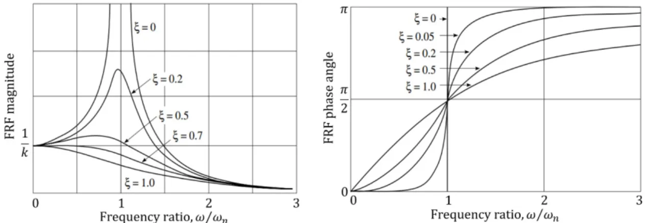
The amplitude of the steady-state response depends on the excitation frequency, 𝜔, and damping ratio, 𝜉. Figure 2.6 shows that the amplitude of the steady-state response approaches a maximum value as the excitation is near the undamped natural frequency, 𝜔𝑛. Moreover, the smaller the damping ratio, the higher the peak.
Figure 2.6 FRF magnitude and phase angle varying with the damping ratio, for a given
undercritically-damped SDOF system.
Periodic loading
In Figure 2.7, a general periodic loading function 𝑓(𝑡) repeats itself in a fixed time period 𝑇, such that 𝑓(𝑡 + 𝑇) = 𝑓(𝑡) for all values of 𝑡.
Figure 2.7 Arbitrary periodic loading. (Source: Clough and Penzien (1993))
This arbitrary periodic loading function can be expanded in an infinite series of sinusoidal functions, called the Fourier series:
𝑓(𝑡) = 𝑎0+ ∑(𝑎𝑛cos 𝑛𝜔𝑡 + 𝑏𝑛sin 𝑛𝜔𝑡) ∞
𝑛=1
(2.20) where 𝜔 = 2𝜋 𝑇⁄ and the Fourier coefficients 𝑎0, 𝑎𝑛 and 𝑏𝑛, are calculated by:
𝑎0 = 1𝑇 ∫ 𝑓(𝑡) 𝑑𝑡 𝑇 0 (2.21) 𝑎𝑛 = 2𝑇 ∫ 𝑓(𝑡) cos 𝑛𝜔𝑡 𝑑𝑡 𝑇 0 , 𝑛 = 1, 2, 3, … (2.22) 𝑏𝑛 = 2𝑇 ∫ 𝑓(𝑡) cos 𝑛𝜔𝑡 𝑑𝑡 𝑇 0 , 𝑛 = 1, 2, 3, … (2.23)
can be given by: 𝑥𝑝(𝑡) =2𝑘 + ∑ 𝜌𝑎0 𝑛sin(𝑛𝜔𝑡 − 𝜃𝑛) ∞ 𝑛=1 , 𝑛 = 1, 2, 3, … (2.25) where 𝜌𝑛 = |𝑥𝑝|
𝑛, representing the magnitude of the vector 𝑥𝑝, which can be found in equation (2.18), and 𝜃𝑛 represents the phase angle, for each 𝑛 (for a full cover on this subject see Clough and Penzien (1993)).
Impulsive loading
The time history of an impulsive load in general is difficult to measure. However, its temporal effect can be quantified. An impulsive load consists in a single impulse of arbitrary form, as illustrated in Figure 2.8, where the duration 𝑡0 is arbitrary small, such that 𝑡0 = 0+.
Figure 2.8 Arbitrary impulsive loading.
Once 𝑓(𝑡) = 0 for 𝑡 > 𝑡0 the impulse-excited motion is equivalent to the free vibration problem, and is solved using equation (2.7) for 𝑡 > 𝑡0, with initial conditions, 𝑥(𝑡0) and 𝑥̇(𝑡0),deduced from the impulse-momentum principle deduced from Newton's second law,
𝐼0 = ∫ 𝑓(𝑡)𝑑𝑡 𝑡0 0 (2.26) respectively, 𝑥(𝑡0) = 𝑥0, 𝑥̇(𝑡0) = 𝑣0+𝑚𝐼0 (2.27)
Therefore, for an undercritically-damped system, initially at rest, the impulse response is: 𝑥(𝑡) =𝑚𝜔𝐼0
𝑑𝑒
−𝜉𝜔𝑛𝑡sin 𝜔𝑑𝑡
(2.28) (Note: See Braun et al. (2002) to further highlights on this matter.)
For the special case, when the considered impulsive load, 𝑓(𝑡), results into a unitary impulse-momentum, 𝐼0, the equation (2.28) returns the IRF-Impulse Response Function, ℎ(𝑡):
ℎ(𝑡) =𝑚𝜔1 𝑑𝑒
−𝜉𝜔𝑛𝑡sin 𝜔𝑑𝑡
(2.29) The IRF represents the unique characteristic of the system/structure, therefore very useful in the dynamical structural analysis field and can be traduced by:
𝑓(𝑡) → [𝑙𝑖𝑛𝑒𝑎𝑟 𝑠𝑦𝑠𝑡𝑒𝑚, ℎ(𝑡)] → 𝑥(𝑡)
In this case, the 𝑓(𝑡) function, can be considered the Dirac's delta function, 𝛿(𝑡), with the following properties: ∫ 𝛿(𝑡 − 𝜏) 𝑑𝑡 = 1 ∞ −∞ (2.30) ∫ 𝑔(𝑡)𝛿(𝑡 − 𝜏) 𝑑𝑡 = 𝑔(𝑡) ∞ −∞ (2.31) such that:
Figure 2.9 Impulse response function for an arbitrary undercritically-damped SDOF system.
where 𝜏 represents a time delay.
For a given loading, 𝑓(𝑡), as represented in Figure 2.10, and considering a portion of the excitation load, 𝑓(𝜏), acting at time 𝑡 = 𝜏, and for a very short time, 𝑑𝜏, as being very short-duration impulse, 𝑓(𝜏) 𝑑𝜏, on the structure, is possible to use the equation (2.29) to obtain the response. Notice that, this equation is exact for impulse with duration 𝑡 = 0+, resulting in approximate results for impulses with finite duration.
Figure 2.10 Derivation of the Duhamel's integral.3
The 𝑥𝑝(𝑡) part of the solution, which does not have any arbitrary constants, can be obtained using the convolution (Duhamel's) integral:
𝑥𝑝(𝑡) = (𝑓 ∗ ℎ)(𝑡) = ∫ 𝑓(𝜏)ℎ(𝑡 − 𝜏) 𝑑𝜏 𝑡
0
(2.32) From where results the impulse response 𝑑𝑥(𝑡), derived from equation (2.29), replacing the 𝑡 variable for (𝑡 − 𝜏):
𝑑𝑥(𝑡) =𝑓(𝜏) 𝑑𝜏𝑚𝜔
𝑑 𝑒
−𝜉𝜔𝑛(𝑡−𝜏)sin 𝜔𝑑(𝑡 − 𝜏) , 𝑡 ≥ 𝜏
(2.33) which is used to obtain the system response:
3 Adaptation from the original, of Clough and Penzien (1993) textbook used to undamped systems, to the
𝑥𝑝(𝑡) =𝑚𝜔1 𝑑∫ 𝑓(𝜏) 𝑒 −𝜉𝜔𝑛(𝑡−𝜏)sin 𝜔𝑑(𝑡 − 𝜏) 𝑑𝜏 𝑡 0 , 𝑡 ≥ 0 (2.34) knowing that ℎ(𝑡 − 𝜏) is represented by:
ℎ(𝑡 − 𝜏) =𝑚𝜔1 𝑑𝑒
−𝜉𝜔𝑛(𝑡−𝜏)sin 𝜔𝑑(𝑡 − 𝜏)
(2.35) However, solving the integral from equation (2.32), in time domain, can be a difficult task, especially when the force function 𝑓(𝑡) is not a simple function. To overcome this fact, numerical and transform methods, Laplace and Fourier, here represented by 𝐿{} and 𝐹{}, respectively, are used in such cases (Note: in following operations, the upper case letters are used for representation in the frequency domain, and lower case letters for representation of time domain). Using domain transformation methods is possible to transform the above integral into an algebraic product which is easier to compute. Then, the solution in the time domain is obtained by performing the inverse transform (frequency to time domain transformation).
Laplace transform
Applying the Laplace transform to the equation (2.2) results on equation, (𝑚𝑠2+ 𝑐𝑠 + 𝑘)𝑋(𝑠) = 𝐹(𝑠)
(2.36) where 𝑋(𝑠) and 𝐹(𝑠) are the Laplace transform (see Annex A1 to get a quick review on Laplace transforms) of 𝐿{𝑥(𝑡)} and 𝐿{𝑓(𝑡)}, respectively, in terms of the Laplace variable 𝑠. Simplifying equation (2.36), and reorganizing it in order to get the response, is obtained:
𝑋(𝑠) = 𝐻(𝑠)𝐹(𝑠) (2.37)
where 𝐻(𝑠), represents the TF-Transfer Function, more precisely the “compliance” and is given by:
𝐻(𝑠) =𝑋(𝑠)𝐹(𝑠) =(𝑚𝑠2+ 𝑐𝑠 + 𝑘)1 (2.38) For the undercritically-damped case, the two complex roots (or “poles”) for the complementary solution of equation (2.36) are given by:
𝑠1,2 = −2𝑚 ± 𝑖𝑐 √ 𝑘𝑚 − (2𝑚)𝑐 2
ℎ(𝑡) =2𝑚𝜔−𝑖 𝑑𝐿 −1{ 1 (𝑠 − 𝑠1) − 1 (𝑠 − 𝑠2)} , 𝑡 > 0 (2.41) Recalling that 𝐿−1{1 (𝑠 − 𝑎)⁄ } = 𝑒𝑎𝑡, ℎ(𝑡) becomes:
ℎ(𝑡) =𝑚𝜔1 𝑑𝑒
−𝜉𝜔𝑛𝑡sin 𝜔𝑑𝑡 , 𝑡 > 0
(2.42) This response, deduced using the Laplace transformation, is the same obtained in equation (2.35), with 𝑡 = (𝑡 − 𝜏), proving the claimed equivalency of the results, using transform and time domain (to further understanding on this subject see Randall (1987) and Braun et al. (2002) textbooks).
Figure 2.11 shows a 3-D representation of the magnitude and phase of the TF, 𝐻(𝑠), for an undercritically-damped system depicting the location of the poles in the complex 𝑠-plane, highlighting the intersection with the imaginary axis, 𝑖𝜔. This intersection represents the FRF, 𝐻(𝑖𝜔).
Figure 2.11 3-D plots representing the transfer function magnitude, |𝐻| (left), and phase angle, 𝜃
(right), in the 𝑠-plane, highlighting the frequency response function, represented by the dashed line.
Fourier transform
Fourier transforms are considered as special cases of the Laplace transforms, when 𝑠 = 𝑖𝜔. It is because of its ability to use the power of modern computers that the use of Fourier transform has clearly overcame the Laplace transform for determining the system response.
Due to the importance of Fourier transform, for practical applications, besides the extended review presented in the Annex A2, it is present next, in this section, the formulas for the (direct) transform:
𝑋(𝑖𝜔) = 𝐹{𝑥(𝑡)} ∫ 𝑥(𝑡)𝑒−𝑖𝜔𝑡 ∞
−∞
𝑑𝑡 (2.43)
which being an even, “two-sided”, function of frequency is usually represented in the format of “one-sided” spectrum using the following conditions (Randall, 1987):
𝑋(𝑖𝜔) = 2𝑋(𝑖𝜔) 𝑖𝜔 > 0
= 𝑋𝑘(𝑖𝜔) 𝑖𝜔 = 0 (2
= 0 𝑖𝜔 < 0
The inverse in given by:
𝑥(𝑡) = 𝐹−1{𝑋(𝑖𝜔)} = ∫ 𝑋(𝑖𝜔)𝑒𝑖𝜔𝑡 ∞
−∞
𝑑𝑓 (2.44)
Note that for practical considerations, from this point, the Fourier transform will be represented using the 𝜔 variable instead of 𝑖𝜔.
Solving the equation (2.32) using Fourier transform:
𝐹{𝑥(𝑡)} = 𝐹{(𝑓 ∗ ℎ)(𝑡)} = 𝐹(𝜔) × 𝐻(𝜔) (2.45) (Note: To see other properties of the Fourier transform see Annex A2)
Returns a system response, 𝐻(𝜔), given by:
𝐻(𝜔) = 𝑋(𝜔)𝐹(𝜔) =𝑚(𝜔 1
𝑛2+ 2𝑖𝜉𝜔𝜔𝑛− 𝜔2) (2.46) It is interesting to note that FRF is the same as the steady-state response of the system to a harmonic exponential excitation, of unit amplitude, and excitation frequency 𝜔 (i.e. 𝑒𝑖𝜔𝑡). This response, is given by:
𝑥𝑠𝑠(𝜔) = 𝐻(𝜔)𝑒𝑖𝜔𝑡= |𝐻(𝜔)|𝑒𝑖(𝜔𝑡−𝜃)
= 1𝑘 1
√(1 − 𝛽2)2+ (2𝜉𝛽)2𝑒𝑖(𝜔𝑡−𝜃), 𝜃 = tan−1( 2𝜉𝛽
1 − 𝛽2) (2.47) where 𝛽 = 𝜔 𝜔⁄ . Using the inverse of Fourier transform is possible to obtain the system 𝑛 response in time domain, 𝑥(𝑡), that is equivalent to the ℎ(𝑡), from equation (2.35), with 𝑡 = (𝑡 − 𝜏):
relation (or contour integral) to perform the improper integral (see Braun et al. (2002) textbook to further information).
Half-power bandwidth
The reader might notice that the response given by equation (2.47) is a recover of the response given by equations (2.18) and (2.19). Let take the change to introduce a new concept regarding the analysis of the FRF amplitude curve, as the one schematised in Figure 2.12 , used to obtain the damping ratio, 𝜉.
Figure 2.12 FRF amplitude, highlighting the resonance, for an arbitrary undercritically-damped SDOF
system. (Source: Clough and Penzien (1993))
There are several methods, based on different properties of the curve in Figure 2.12, which can be used to deduce the damping ratio. However, the most popular method is the “half-power bandwidth” method (or band-width method, or even -3db method) whereby the damping ratio is
determined, at a resonance4 peak, from the frequency at which the response amplitude 𝜌 is reduced to the level 𝜌𝑚𝑎𝑥⁄ . √2
Deduced from Figure 2.12, is possible to obtain the following relation, for small values of damping (Clough and Penzien 1993):
𝜉 =𝛽𝛽2− 𝛽1
2+ 𝛽1 (2.49)
Since the 𝛽 = 𝜔 𝜔⁄ , and 𝜔 = 2𝜋𝑓, is possible to obtain the damping ratio in order to the 𝑛 frequency, 𝑓, which is usually more convenient for practical cases:
𝜉 =𝑓2− 𝑓1
𝑓2+ 𝑓1 (2.50)
Power spectral density
Whenever a vibrating system is excited by random force(s), the response is also random. One of the methods available to obtain the system response is the direct use of the basic excitation/response relation for PSD-Power Spectral Density.
Whenever the response is stationary, its PSD, represented by 𝑆𝑋𝑋(𝜔) can be predicted in terms of the excitation PSD, represented by 𝑆𝐹𝐹(𝜔), and relevant complex frequency response H, using the basic relation:
𝑆𝑋𝑋(𝜔) = |𝐻2(𝜔)|𝑆𝐹𝐹(𝜔) (2.51) Considering an arbitrary waveform, 𝑥(𝑡), to represent a stationary random process, which is represented only over a finite interval, − 2 𝑠⁄ < 𝑡 < 2 𝑠⁄ , its PSD (𝑆𝐹𝐹(𝜔)) can be deduced from: |𝑥(𝑡)2| = ∫ 𝑆 𝑋𝑋(𝜔) 𝑑𝜔 ∞ −∞ (2.52) where the function:
𝑆𝑋𝑋(𝜔) ≡ lim𝑠→∞ |∫2 𝑠⁄ 𝑥(𝑡) 𝑒−𝑖𝜔𝑡𝑑𝑡 −2 𝑠⁄ | 2 2𝜋𝑠 (2.53)
4 Resonance is the condition that results the maximum steady-state response amplitude, assumed to occur when the
frequency of the applied loading equals the undamped natural vibration frequency. Knowing that for low values of damping the maximum steady-state response amplitude occurs at a frequency ratio slightly less than unity.
𝑅𝑥𝑥(𝜏) = ∫ 𝑆𝑥𝑥(𝜔)𝑒𝑖𝜔𝜏𝑑𝜔 ∞
−∞
(2.55) (Note: To properly check how the presented equations are deducted see the following textbooks: Clough and Penzien (1993); Braun et al. (2002))
Autocorrelation function, 𝑅𝑥𝑥(𝜏), in its turn, it is a special case of the cross-correlation function, 𝑅𝑥𝑦(𝜏) where two signals, 𝑥(𝑡) and 𝑦(𝑡), are correlated using the following equation:
𝑅𝑥𝑦(𝜏) = (𝑥 ⋆ 𝑦)(𝜏) =1𝑇 ∫ 𝑥(𝑡)𝑦(𝑡 + 𝜏) 𝑑𝑡 𝑇
0
(2.56)
Figure 2.13 shows schematic representations of autocorrelation, 𝑅𝑥𝑥(𝜏), cross-correlation, 𝑅𝑥𝑦(𝜏), at the same time, highlighting the “similarities” with convolution function, previously referred.
Figure 2.13 Schematic representation of Convolution, Cross-correlation and Autocorrelation operations.
(Source: wikipedia.org)
Transforming 𝑅𝑥𝑦(𝜏) using the Fourier transform, similarly to what is done for 𝑅𝑥𝑥(𝜏) in equation (2.54) will result in an important physical quantity in the field of dynamic analysis named Cross-Spectral Density (CSD), represented by
5 A process is defined as ergodic when any average obtained with respect to time 𝑡 along any member 𝑟 of the
ensemble is exactly equal to the corresponding average across the ensemble at an arbitrary time 𝑡 (Clough and Penzien 1993).
𝑆𝑋𝑌(𝜔) = 𝐹{𝑅𝑥𝑥(𝜏)} = ∫ 𝑅𝑥𝑦(𝜏)𝑒−𝑖𝜔𝜏𝑑𝜏 ∞ −∞ = ∫ ∫ 𝑥(𝑡)𝑦(𝑡 + 𝜏)𝑒−𝑖𝜔𝜏𝑑𝜏𝑑𝑡 ∞ −∞ ∞ −∞ (let 𝑡1 = 𝑡 + 𝜏) = ∫ 𝑥(𝑡)𝑒𝑖𝜔𝑡𝑑𝑡 ∫ 𝑦(𝑡 1)𝑒−𝑖𝜔𝑡1𝑑𝑡1 ∞ −∞ ∞ −∞ = 𝑋∗(𝜔)𝑌(𝜔) (2.57)
Where 𝑋∗(𝜔) is the complex conjugate (𝑋(−𝑖𝜔) = 𝑋∗(𝑖𝜔)).
Note that the function 𝑆𝑋𝑌(𝜔) result in the two-sided cross spectrum. Therefore, the same approach used for the Fourier transform, in equation (2.43), is used to obtain the one-sided spectrum:
𝐺𝑋𝑌(𝜔) = 2𝑆𝑋𝑌(𝜔) 𝜔 > 0
= 𝑆𝑋𝑌(𝜔) 𝜔 = 0 (2.57a)
= 0 𝜔 < 0
To obtain the one-side 𝐺𝑋𝑋(𝜔) spectrum the same procedure is used. Having established the previous concepts, and knowing that:
𝑆𝑋𝐹(𝜔) = 𝑆𝐹𝑋∗ (𝜔) (2.58) Silva and Maia (1999) wrote that it is possible to go through a series of mathematical manipulations and demonstrate that:
𝑆𝐹𝑋(𝜔) = 𝐻(𝜔)𝑆𝐹𝐹(𝜔) (2.59) 𝑆𝑋𝑋(𝜔) = 𝐻(𝜔)𝑆𝑋𝐹(𝜔) (2.60) Equations (2.59) and (2.60) represent and adequate relationships that enable the frequency response function of a system to be determined from knowledge of the input force and output response characteristics.
of DOFs. Figure 2.14 has schematised a MDOF system, with 𝑛 number of DOFs.
Figure 2.14 Damped MDOF system.
The motion of damped MDOF systems is governed by a set of simultaneous differential equations. Using [𝑚] as the mass matrix, [𝑐] the damping matrix, and [𝑘] the stiffness matrix, the equation to describe motion of a damped MDOF system becomes:
[𝑚]{𝑥̈(𝑡)} + [𝑐]{𝑥̇(𝑡)} + [𝑘]{𝑥(𝑡)} = {𝑓(𝑡)} (2.61) Developing the equation (2.61) for the damped MDOF system schematised in Figure 2.14, will results in the next mass ([𝑚]), damping ([𝑐]), and stiffness ([𝑘]) matrices:
[𝑚] = [ 𝑚1 0 ⋯ 0 0 𝑚2 ⋯ 0 ⋮ ⋮ ⋱ ⋮ 0 0 ⋯ 𝑚𝑛 ] (2.62a) [𝑐] = [ (𝑐1+ 𝑐2) −𝑐2 ⋯ 0 −𝑐2 (𝑐2+ 𝑐3) ⋯ 0 ⋮ ⋮ ⋱ ⋮ 0 0 ⋯ (𝑐𝑛+ 𝑐𝑛+1) ] (2.62b) [𝑘] = [ (𝑘1+ 𝑘2) −𝑘2 ⋯ 0 −𝑘2 (𝑘2+ 𝑘3) ⋯ 0 ⋮ ⋮ ⋱ ⋮ 0 0 ⋯ (𝑘𝑛+ 𝑘𝑛+1) ] (2.62c)
and displacement {𝑥(𝑡)}, velocity {𝑥̇(𝑡)}, acceleration {𝑥̈(𝑡)}, and force {𝑓(𝑡)} vectors: {𝑥(𝑡)} = { 𝑥1(𝑡) 𝑥2(𝑡) ⋮ 𝑥𝑛(𝑡) } , {𝑥̇(𝑡)} = { 𝑥̇1(𝑡) 𝑥̇2(𝑡) ⋮ 𝑥̇𝑛(𝑡) } , {𝑥̈(𝑡)} = { 𝑥̈1(𝑡) 𝑥̈2(𝑡) ⋮ 𝑥̈𝑛(𝑡) } , {𝑓(𝑡)} = { 𝑓1(𝑡) 𝑓2(𝑡) ⋮ 𝑓𝑛(𝑡) } (2.62d)
2.1.2.1 SDOF/MDOF systems equivalencies
Knowing that previous mathematical manipulation approaches, used for the damped SDOF system, can be used to solve the differential equations of motion for damped MDOF system, let just make now a brief resume on some relevant points, concerning damped MDOF system response.
The Laplace transform
Solving equation (2.61) using the Laplace transform:
([𝑚]𝑠2 + [𝑐]𝑠 + [𝑘]){𝑋(𝑠)} = {𝐹(𝑠)}
(2.63) where 𝑋(𝑠) and 𝐹(𝑠) are the Laplace transform 𝐿{𝑥(𝑡)} and 𝐿{𝑓(𝑡)}, respectively. The unique characteristic of the system, TF-Transfer Function (in this particular case “compliance”):𝐻(𝑠) = ([𝑚]𝑠2+ [𝑐]𝑠 + [𝑘]), can be achieved by:
𝐻(𝑠) ={𝑋(𝑠)}{𝐹(𝑠)} (2.64)
Fourier transform
As demonstrated early, the TF in the Fourier domain is designed FRF-Frequency Response Function, when 𝑠 = 𝑖𝜔. So, the “compliance” transfer function is represented:
𝐻(𝑖𝜔) ={𝑋(𝑖𝜔)}{𝐹(𝑖𝜔)} (2.65) Usually vibration is measured in terms of motion. Therefore the corresponding FRF may be presented in terms of displacement, velocity and acceleration variables. The terminology for each type of these response variables is:
𝐺(𝑖𝜔) =𝑑𝑖𝑠𝑝𝑙𝑎𝑐𝑒𝑚𝑒𝑛𝑡 𝑟𝑒𝑠𝑝𝑜𝑛𝑠𝑒𝑓𝑜𝑟𝑐𝑒 𝑒𝑥𝑐𝑖𝑡𝑎𝑡𝑖𝑜𝑛 = Compliance (2.66) 𝑌(𝑖𝜔) =𝑣𝑒𝑙𝑜𝑐𝑖𝑡𝑦 𝑟𝑒𝑠𝑝𝑜𝑛𝑠𝑒𝑓𝑜𝑟𝑐𝑒 𝑒𝑥𝑐𝑖𝑡𝑎𝑡𝑖𝑜𝑛 = Mobility (2.67) 𝐴(𝑖𝜔) =𝑎𝑐𝑐𝑒𝑙𝑒𝑟𝑎𝑡𝑖𝑜𝑛 𝑟𝑒𝑠𝑝𝑜𝑛𝑠𝑒𝑓𝑜𝑟𝑐𝑒 𝑒𝑥𝑐𝑖𝑡𝑎𝑡𝑖𝑜𝑛 = Accelerance (2.68)
Figure 2.15 Exemplificative response of a MDOF system to a transient loading in the time domain (left)
– acceleration – and, the respective frequency par, in the Fourier domain (right) – accelerance. However, there are other physical quantities derived from FRFs, which are used in some dynamic analysis. These relations, possible to obtain from measuring systems, are resumed in Table 2.2, which will be further discussed in this chapter (section 2.3.2.1).
Note that this text intends to give a brief review on relevant subjects. Therefore, to obtain a detailed cover on this subject, see textbooks: Clough and Penzien (1993) and Silva and Maia (1999).
2.2 Signal processing
“Signal processing is the enabling technology for the generation, transformation, extraction, and interpretation of information. It comprises the theory, algorithms with associated architectures and implementations, and applications related to processing information contained in many different formats broadly designated as signals. Signal processing uses mathematical, statistical, computational, heuristic, and/or linguistic representations, formalisms, modelling techniques and algorithms for generating, transforming, transmitting, and learning from signals” (IEEE Signal Processing Society, 2012).
In last decades signal processing have played an important role in our lives, being present in almost every application domains (from image to sound processing passing by financial signal processing and many other applications). However, the appearance of signal processing goes back
far behind in past. In a historical background Oppenheim et al. (1998) found that scientists and engineers, since the invention of calculus in the 17th century, have developed models to represent
physical phenomena in terms of functions of continuous variables and differential equations. Numerical techniques have been used to solve these equations when analytical solutions are not possible. Oppenheim et al. (1998) refer that Newton used finite-difference methods that are special cases of some discrete-time systems and Goldstine (1977) attributes to Carl Friedrich Gauss, in a work about interpolation of orbits of celestial bodies (presumed dated from 1805), the discover of an algorithm similar to the Fast Fourier Transform algorithm, later reinvented by Cooley and Tukey (1965).
IEEE Signal Processing Society (2010) assumes signal processing as an essential technology, which integrates contributions of several scientific and engineering disciplines, to achieve profitable tools. In the context of the present work, signal processing becomes a fundamental tool used to predict structural dynamic behaviour, using signals from a wide range of sensors typology.
2.2.1 Signal acquisition
The term signal is used to define the observed data, which is representing a physical phenomenon, as a continuous-time function. Temperature oscillations, pressures changes, voltage variations, water level, etc., are some examples of signals. Physical phenomenon in observation is traduced by a continuous (analogue) signal (see Figure 2.16-A to get an example of a typical continuous signal). However, in order to digitally process analogue signals it is necessary to convert them into digital form. In the end, digital signals are obtained by sampling the analogue signal into discrete values. Randall (1987) defines sampled continuous-time functions as “Time-Series” functions, representing sequences of discrete values equi-spaced in time, i.e., sampling a signal is, simply, to record it from time to time, at a given sampling rate6. Figure 2.16-B shows an example of discrete
signal, sampled at every ∆ seconds.
6 Sampling rate is the frequency at which the signal samples are taken, for instance, a signal with 10 samples per
Figure 2.16 Typical examples of signals: (A) Continuous (analogue) signal; (B) Discrete signal (digital), sampled at every ∆ seconds7
.
In practice, analogue signals, representing the physical phenomenon, are transformed into electrical signals through the use of special transducers, commonly referred as sensors. Sensors interprets the physical phenomena and convert them into electrical quantities allowing the electronic processing. Table 2.1 presents some examples of existent sensors and its physical phenomenon target. Regardless the sensor type to be used, this, analogue-to-digital (A/D), translation, is done using data acquisition (DAQ) systems.
Table 2.1 Sensor and physical phenomenon target.
Sensor Phenomenon
Thermocouple, RTD, Thermistor Temperature
Photo Sensor Light
Microphone Sound
Strain Gage, Piezoelectric Transducer Force and Pressure Potentiometer, LVDT, Optical Encoder Position and Displacement
Accelerometer Acceleration
Vibrometer Velocity
pH Electrode pH
The objective of a DAQ system is to collect and record data from physical phenomena, converting analogue waveforms into digital values for posterior signal processing. Figure 2.17 shows a schematic diagram of a general DAQ system.
Figure 2.17 Schematic diagram of a general data acquisition system. A/D, analogue-to-digital8
.
DAQ systems include:
Sensor (or transducer) that convert physical parameters to electrical signals;
Conditioner that modifies the signal from the sensor to provide signals suitable for the analogue-to-digital (A/D) converter;
A/D converter, which convert conditioned sensor signals to digital values; And a Recorder, used to store the collected data.
2.2.2 Signal types
In practice, there are several types of signal to be analysed. Signal type has influence on the type of analysis to be performed and also on the choice of analysis parameters. Randall (1987) considers that the most fundamental division of signals is into stationary and non-stationary signals. Figure 2.18 represents the proposed division.
Figure 2.18 Signal types. (Source: Randall (1987))
Stationary deterministic
Stationary deterministic signals are those that can be exactly defined using a mathematical formula. Inside this class are the periodic and the quasi-periodic signals. Periodic signals are those whose waveforms repeats exactly at regular time intervals. There are several examples of periodic waveforms, from the simplest example, the sinusoidal signal, present in Figure 2.19, to more complex signals as the one depicted in Figure 2.7.
Figure 2.19 Sinusoidal signal with a period 𝑇 [s].
The quasi-periodic are those signals which seams periodic but, in fact, they are not. Randall (1987) gives the example of an aircraft turbine with two independent rotating shafts, which produce quasi-periodic signals by the mixture of two or more independent set of harmonics. And Shin and Hammond (2008) present the example of the “hum noise”9, which is represented in Figure 2.20.
Figure 2.20 Hum noise signal. (Source: Shin and Hammond (2008))
Stationary random
In contrast with the deterministic signals, random signals cannot be represented by any mathematical formula. However, being a stochastic process whose joint probability distribution does not change when shifted in time. Parameters such as the mean and variance, if they are present, also do not change over time and do not follow any trends. A typical example of such signals is the “white noise” signal and is presented in Figure 2.21.
9 The Hum is a phenomenon, or collection of phenomena, involving widespread reports of a persistent and invasive
Figure 2.21 White noise signal.
Pseudo-random
Pseudo-random signal are a particular type of periodic signal, with large periodic 𝑇, sometimes used to simulate random signals.
Transient
Transient signals, are those signals that represent a transitory state, usually meeting the conditions: 𝑥(𝑡) = 0 (𝑡 = 0 , 𝑡 = +∞). Typical examples of such signals, in SDA, are the resultant from the impact testing (properly covered further in section 2.3.2.2) on structures used to obtain the FRF. Figure 2.22 shows the transient signal resultant from the impact and the respective read obtained by the accelerometer.
Figure 2.22 Typical example of transient signals.
Non stationary
Non-stationary signals covers all signals that does not meet the conditions of stationary ones. This means that parameters such as the mean and variance change over time and do not follow any trends. A typical example of such signals are depicted next:
Figure 2.23 Typical example of non-stationary signals. (Source: Shin and Hammond (2008))
2.3 Theoretical introduction to the problem
In general, the purpose of signal processing in SDA field is the extraction of information from a signal, especially when it is difficult to obtain relevant information from a simple direct observation. Extracting information from a signal has three key stages: (i) acquisition, (ii) processing, (iii) interpretation. Once the focus of this work is related to “development of a signal processing tool for the post-processing of structural dynamics results obtained through the application of the finite element method” a special attention to stages (ii) processing and (iii) interpretation is given next, while the (i) acquisition, mainly related with experimental implementation, will remain briefly reviewed as it was made in previous section 2.2.1.
As claimed in the Signal acquisition section, in order to digitally process analogue signals is necessary to convert them into digital form. This transformation create continuous signals into discrete ones. Therefore, a set of discrete formulas (deduced from the continuous “pair”) must be defined in order to allow the signal processing of discrete signals.
A wide range of authors, such He and Fu (2001), Marwala (2010), Kessle et al. (2011), Khennane (2013) and others, claim that many applications of modern SDA rely their success almost entirely upon having accurate mathematical model for representing the dynamic of structures. These models can be obtained using FEM, which derives the FE model in form of mass, damping and stiffness matrices. The resultant model, can be used for further engineering applications such as sensitivity analysis, prediction of the dynamic response due to structural changes, materials selection, material fatigue prediction, etc.... However, given the complexity and uncertainty of real structures, hardly the FE model results in a truly representation. Friswell and Mottershead (1995) wrote a list with the reasons for the discrepancy between FE model data and measured data: (i) model structure errors, which may result from the difficulty in modelling damping, joints, welds and edges; (ii) model order errors, which may result from the difficulty in