Genetic Algorithm and Variational Method to Identify Initial Conditions:
Worked Example in Hyperbolic Heat Transfer
L.B.L. SANTOS1*, L.D. CHIWIACOWSKY2 and H.F. CAMPOS-VELHO3
Received on December 4, 2012 / Accepted on May 20, 2013
ABSTRACT.The identification of initial condition from measurements at a given time is a hard inverse problem, and it can be applied to evaluate the robustness of inversion strategies. Relevant scientific is-sues are related with estimation of initial condition: cosmology and data assimilation are good examples. Two different inversion methods are employed to identify initial condition for parabolic and hyperbolic differential equations: Genetic Algorithm and Variational Method. The heat transfer process was selected to be used in our tests. A harder inversion is verified on hyperbolic case. Both inverse methods were ef-fective: the numerical difference between the inverse solution was not significant, although the variational method presented a smoother inversion. The inversion obtained with the variational method presented lower processing time.
Keywords:initial condition identification, epidemic genetic algorithm, variational method, parabolic and hyperbolic differential equation.
1 INTRODUCTION
Partial differential equations (PDE) are frequently used to express the mathematical models for natural phenomena. Let be a linear PDE:
Aux x +Bux y+Cuy y+Dux+Euy+Fu+G=0
where the coefficients A, B, C, D, E, F are functions such that A2(x,y)+ B2(x,y)+ C2(x,y) = 0, and G = G(x,y)is a real function defined on an open set. The PDE can be classified looking at the quantity = B2(x,y)−4A(x,y)C(x,y). A PDE is classified as parabolic if <0, elliptic if=0, and hyperbolic if >0.
*Corresponding author: Leonardo B.L. Santos
1Programa de Mestrado em Computac¸˜ao Aplicada – CAP, Instituto Nacional de Pesquisas Espaciais – INPE. E-mail: [email protected]
Elliptic equations are usually linked to the equilibrium relations, while parabolic and hyperbolic equations are associated with evolution processes. Parabolic and hyperbolic equations have in-finity and finite velocities for the signal propagation, respectively.
For the solution of a PDE, it is necessary to specify the properties of the system (system coeffi-cients and heterogeneous terms), with the initial and boundary conditions. This solution charac-terizes the forward problem. Inverse problem is expressed when the PDE solution is measured or specified, and we are interested to determine some property: coefficients, forcing term, boundary or initial condition. Considering the cause-effect pair, the forward problem is to determine effects from the known causes, while the inverse problem deals with the identification of one (or some) cause(s) from the measured or desired effects [2]. The latter inverse problem is also known as inverse design or optimal experiment design.
Initial condition determination is a crucial issue, for example, in cosmology, since different ini-tial conditions produces different models of the cosmos. Therefore, in order to have a good understanding of the cosmos formation or its evolution, the estimation of initial condition is necessary [9]. Other application where the initial condition identification is an essential proce-dure is the data assimilation [13], one of most important topics of research, and it is employed for the numerical weather prediction, ocean circulation, environmental prediction, and ionospheric dynamics.
The focus of the present paper is to determine initial condition, where inverse solution is iden-tified by two different methodologies: genetic algorithm with epidemic operator (GAE), and variational approach.
The inverse schemes are tested on the heat transfer processes. From the conservation principles and from the Fourier’s law, the heat conduction problem is formulated generally by a parabolic equation. A modification on the Fourier’s law is done to model the thermal signal with finite speed, implying in a hyperbolic equation for the heat propagation [5]. The latter equation de-scribes a damped wave, with similar behavior of mechanical or electromagnetic waves in the attenuating medium.
Inverse problems can be formulated as an optimization problem with constraints, where the ob-jective function is expressed as the squared difference between the measured (desired) property and the computed solution of a PDE. The constraints could be an additional property on the esti-mated quantity (e.g. smoothness or regularized solution), or the PDE itself. The latter condition is employed in the variational approach. The Alifanov’s formulation for the variational approach uses the conjugate gradient method (CGM) for solving the optimization problem [1]. The opti-mum solution can also be computed by applying techniques based on artificial intelligence, as genetic algorithm, a stochastic global search method.
the initial condition signal is exponentially attenuated in the parabolic equations. For dealing with hyperbolic systems, a hybrid method was proposed [3, 7, 17], where the genetic algorithm, with epidemic operator [16], is combined with the CGM. The GAE is used to find a solution in the attraction basin. Following, the CGM is activated to perform a local search to compute the final inverse solution.
There are some results in the literature to compute inverse solutions in the hyperbolic heat trans-fer. However, there is no results estimating initial condition using the Alifanov’s approach: Huang and Hsin-HsienWu [10] apply the Alifanov’s approach to estimate the boundary con-dition; Huang and Lin [11] apply Alifanov’ s approach to estimate simultaneously two boundary conditions; Huang and Lin [12] seek source term estimation by Alifanov’s approach; Das et al. [8] employ a genetic algorithm for simultaneous estimation of the extinction coefficient and the conduction-radiation parameter.
For mathematical models with diffusion process, the inverse problem of initial condition iden-tification is harder than determine boundary condition. On the other hand, the effect of noise in the hyperbolic problem is more significant than in the parabolic formulation, because the ini-tial condition signal is propagated to entire domain. Therefore, the reconstruction of the iniini-tial condition for the wave equation for the heat transfer is a good test problem to evaluate inversion techniques.
The goal of this paper is to present the physical description, mathematical formulation, numer-ical solution of the forward problem for heat transfer considering both infinity (standard heat conduction) and finite (wave equation) speed of signal, and lastly to show results of the inversion techniques when estimating initial condition for these two test problems.
2 FORWARD PROBLEM SOLUTIONS
The principle of the energy conservation for the heat transport in a solid homogeneous and isotropic material without source term implies that the variation of the temperature is given by the divergence of heat flux inside of a given domain:
ρc∂T(r,t)
∂t + ∇ · −
→q (r,t)=0, (2.1)
whereT is the temperature,ρ is the density, cis the heat capacity and−→q is the heat flux at specific positionrand timet.
The heat conduction equation is derived from the Fourier’s law of heat flux. The generalized Fourier’s law for the heat flux is expressed as
τ∂ − →q (r,t)
∂t + −
→q(r,t) = −κ∇T(r,t);
(2.2)
τ =
=0 for standard Fourier’s law,
whereκis the thermal conductivity coefficient (a material property) andτ is the relaxation time, which indicates a no-null finite time of heat accumulation for changing the thermal flux.
The standard form of Fourier law is a constitutive relation expressed by the temperature gradient multiplied by the thermal conductivityκand assumingτ =0 in Eq. (2.2):
−
→q(r,t)= −κ∇T(r,t) . (2.4)
The parabolic heat conduction transfer is derived combining the standard constitutive relation above with the conservation principle (2.1). The wave equation for the heat transfer is obtained by combining the generalized Fourier’s law (2.2) and the energy conservation law (2.1) [5]:
τ∂
2T(x,t)
∂t2 +
∂T(x,t) ∂t −
κ ρc∇
2T(x,t)=
0. (2.5)
In the parabolic caseτ = 0, and in the hyperbolic problem the formulation works with an upper-limit for the no-null finite speed of the propagation signal defined as:
a =
κ
ρcτ . (2.6)
The hyperbolic approach is relevant when high ratios of heat transfer on short time period, very low temperature, and electromagnetic radiation of high intensity are involved [15]. Depending on the type of the material, the value ofτ is different with values, for homogeneous materials, from 10−10 to 10−8s for gases, and from 10−12to 10−10s for solids and dielectric liquids, but different values are also reported in the literature [14].
For our test problem, a 1D forward problem to the heat wave can be defined. Let T(x,t)∈C2
defined in the domain≡x ×t, wherex = [0,L]andt = [0,tf), such as:
τ∂
2T(x,t) ∂t2 +
∂T(x,t) ∂t −
κ ρc∇
2T(x,t) = 0, x∈
x, t ∈t ; (2.7)
T(x,0) = f(x) , x∈x, (2.8) ∂T(x,0)
∂t = 0, x∈x, (2.9)
∂T(0,t)
∂x = 0, t∈t, (2.10)
∂T(L,t)
∂x = 0, t∈t. (2.11)
3 INVERSE SOLUTIONS
In this work two different methods are proposed for the initial condition identification related to both parabolic and the hyperbolic heat transfer. The inverse problem solution is sought by using methods of two different classes: stochastic and deterministic. In one hand, the Genetic Algorithm is a bio-inspired stochastic method. On the other hand, the Variational method (or Ali-fanov’s iterative regularization approach) is a deterministic scheme where the conjugate gradient method is used with the adjoint equation.
The solution of the inverse heat conduction problem employing the techniques considered here, is based on the minimization of a well-posed functional form given by:
J[f(x)] =
M
m=1 t=t f
t=0
[T(xm,t)f(x)−TEx p(xm,t)]2dt (3.12)
where M is the number of temperature sensors,T(xm,t)f(x) is the temperature computed
us-ing the recovered initial condition, andT(xm,t)Ex pis the measured temperature at each sensor location.
3.1 Stochastic Approach – The Genetic Algorithm
Concerning the GA implemented here and applied for the solution of the inverse problem of ini-tial temperature estimation, it operates on a fixed-sized population which is randomly generated initially. Each member of the population corresponds to a particular initial temperature profile
f(x), which is encoded as a fixed-length and real valued string. Following, the evolutionary operators employed in this work are presented.
– Tournament Selection
best:=rand; worst:=rand; val:=0.75; if (ran<val) then
position:=best; else
position:=worst; endif
whererand is a random number from[0,1)with uniform distribution,best is a best fitness individual andworstis a worst fitness individual.
– Geometrical Crossover
This crossover operator breeds only one offspring from two parents. From the parentsxi andyi the offspring is represented by
zi =xµi yi1−µ, (3.13)
– Non-uniform Mutation
This mutation operator is defined by
xi′=
⎧ ⎨
⎩
xi+ △(t,lsup−xi) if a random binary digit is 0,
xi − △(t,xi−lin f) if a random binary digit is 1,
(3.14)
such as
△(t,y)=y 1−rand(1−Ht) b
,
whererand is a random number from[0,1)with uniform distribution,H is the maximal gen-eration number,tis the current generation number, andbis a system parameter determining the degree of non-uniformity.
– Epidemical Strategy
Beyond the standard genetic operators described before, a new operator called epidemical has been used. This operator is activated when a specific number of generations is reached without improvement of the best individual. When it is activated, all the individuals are affected by a plague, and only the fittest individuals (e.g. the first 5% fittest individuals in the population)
survive. The remainingdieand their place is occupied by new individuals with new genetic variability, such as immigrants arriving, to continue the work that was done before by others.
3.2 Deterministic Approach – The Variational method
The variational method is an efficient and elegant option to find inverse solutions. Its implemen-tation uses several steps: forward problem, sensitivity problem, adjoint problem and gradient equation, and conjugate gradient method. The functional form to be minimized is that defined in eq. (3.12). A description of the implementation steps is presented.
3.2.1 The sensitivity problem
The sensitivity problem is derived from the forward problem, by applying a small perturbation on the initial condition, resulting f(x)+f(x). This perturbation implies in a modification on the answer of the forward problem,T(x,t)+T(x,t). The sensitivity problem is obtained by intro-ducing the perturbed quantities in the forward problem and subtracting it from the unperturbed problem. Following, the respective sensitivity problem is defined:
τ∂
2T(x,t) ∂t2 +
∂T(x,t) ∂t −
k
ρc∇
2T(x,t) = 0, x∈
x, t ∈t; (3.15)
T(x,0) = f(x), x ∈x; (3.16)
∂T(x,0)
∂T(0,t)
∂x = 0, t ∈t; (3.18)
∂T(L,t)
∂x = 0, t ∈t. (3.19)
In the case of parabolic heat conduction, the equations are the same, but takingτ=0.
3.2.2 The adjoint problem and the gradient equation
For the adjoint problem definition, the forward problem is used as a constraint for the optimiza-tion problem to be solved. The funcoptimiza-tional form (3.12) is modified by adding the constraint and using a new functionλ(x,t), called the Lagrange multiplier [1]. Thus, the equation of forward problem is multiplied by the Lagrange multiplier (or adjoint function)λ(x,t), integrating the resulting expression over time and space domain and adding the result to the functional given by (3.12). Performing integration by parts and using the boundary conditions and the sensitive problem, is possible to construct the following adjoint problem:
τ∂ 2λ(x,t)
∂t2 +
∂λ(x,t) ∂t +
κ ρc∇
2λ(x,t)=
= −2 M
m=1 tf
0
[T(xm,t)−TEx p(xm,t)]dt, x∈x, t ∈t; (3.20)
λ(x,tf)=0, x∈x. (3.21)
The term left in the development of the differential of the Lagrangian is used to determine the gradient equation, respectively defined as:
J′(x,0)= J′(x)= 1 tf
λ(x,0)−τλ(˙ x,0). (3.22)
In the case of parabolic heat conduction, again, the equations are the same, but takingτ=0.
3.2.3 The stopping criterion
If the problem contains no measurement errors, one can use the customary stopping criteria
J(fk+1) < ǫ∗, (3.23)
whereǫ∗ is a small specified number. However, in practical applications, measurement errors are always present; therefore the discrepancy principle as described below should be used to establish the stopping criterion [1].
It is assumed that the temperature residuals may be approximated by
whereσ is the standard deviation of the measurement errors, assumed the same for all sensors and measurements.
Introducing this result into equation (3.12) we obtain
M
m=1 tf
0
σ2dt=Mσ2tf ≡ǫ2. (3.25)
Then the discrepancy principle for the stopping criterion is taken as
J fk+1(x)< ǫ2. (3.26)
4 RESULTS AND DISCUSSIONS
Results are shown for estimating the initial condition (a triangular profile) for the diffusion and wave heat transfer problems. The estimation is computed using two methods: genetic algorithm and variational approach. The parameters used to solve the forward problem wereNx =101 grid points,tf = 0.15s with 250 time-steps. For emulating the experimental data, a multiplicative white Gaussian noise was associated to the computed temperature.
The genetic algorithm was executed with 2000 as a maximum number of iterations, population with 100 individuals, mutation ratio 20%, and the epidemic operator is activated when the best solution does not change for 10 iterations. The action of the epidemic operator preserves the 5% of the best individuals, and the rest of the population is substituted by other randomly generated. In the variational approach, the conjugate gradient is executed up to 200 iterations or if the Morozov’s discrepancy principle is reached. On average, each iteration of GA requires 0.19 sec., and 0.1 sec. for the variational method, on the following hardware: processor IntelCeleron, 2133 Mhz, 1GB DDR2 memory.
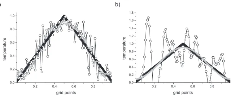
Figure 1(a) shows the initial condition estimated by the GA, obtained with and without the di-crepancy principle. The inversions are similar to those found in the literature [2]. The numerical experiments were carried out with 0.5% of noise level. Better results are achieved when the discrepancy principle is used as stopping criterion.
Results for variational method are shown in Figure 1(b), with the same level of noise, using and not using the Morozov’s stopping criterion. If the Morozov’s principle is not applied the inverse solution is corrupted by the noise. With the application of discrepancy criterion only three iterations are necessary to get the inverse solution.
Inversion for hyperbolic heat transfer using GA is displayed by Figure 2(a), with and without application of the discrepancy principle. The presence of noise has a stronger impact on the hyperbolic model: for the hyperbolic problem the level of noise was 0.1% – 5 times lower than the parabolic example. Figure 2(b) shows the inversion for the hyperbolic heat transfer computed by the variational method with and without the Morozov’s stopping criterion.
Figure 1: Inverse solutions for parabolic heat transfer by GA (a) and VM (b). The black squares show the true temperature profile, white circles for the inversion without regularization and the Morozov’s principle was not applied, and gray triangles present the inverse regularized solution with discrepancy principle employed.
Figure 2: Inverse solutions for hyperbolic heat transfer by GA (a) and VM (b). The black squares show the true temperature profile, white circles for the inversion without regularization and the Morozov’s principle was not applied, and gray triangles present the inverse regularized solution with discrepancy principle employed.
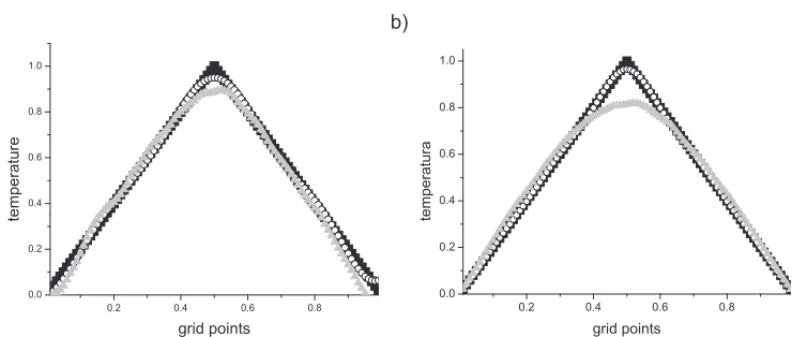
Figure 3: Inverse solutions for heat transfer throught VM for the parabolic (a) and hyperbolic (b) problems, on both cases applying the Morozov’s principle. The black squares show the true temperature profile, white circles the inversion considering noiseless experimental data and the gray triangles present the inverse solution for data with high noisy level.
5 CONCLUSIONS AND FINAL REMARKS
Two methodologies (Genetic Algorithm and Variational Method) to compute inverse solutions were applied to identify the initial condition on two class of partial differential equations prob-lems (Parabolic and Hyperbolic). Both methodologies were effective to compute the inverse solution. In despite of several results in the literature to compute inverse solutions in the hyper-bolic heat transfer with a number of different methods, and recovery initial conditions on a lot of problems, to the best of author’s knowledge, there are no results estimating initial condition on this hyperbolic problem, and, in this case, using the Alifanov’s approach [4].
The epidemic GA was more time consuming than the variational method. The Morozov’s dis-crepancy principle was showed to be a necessary stopping criterion. Smoother inverse solutions were obtained with variational method. Although, the variational method has presented a bet-ter performance (fasbet-ter convergence, and smoother inversions), the variational formulation is required (sometimes is difficult to derive this formulation, if possible), and the method is only applicable for differentiable functions.
The hyperbolic case is more sensitive related to the experimental noise than the parabolic formu-lation, since the propagation of the initial condition and its persistence during the process for a longer time contributes to corrupt the solution in a harder way.
m´etodos distintos s˜ao empregados para identificar condic¸˜oes iniciais para equac¸˜oes parab´o-licas e hiperb´oparab´o-licas. O processo de transferˆencia de calor foi selecionado em nossos testes. A invers˜ao mostrou-se mais dif´ıcil para o caso hiperb´olico. Ambos os m´etodos de invers˜ao foram efetivos: as diferenc¸as num´ericas entre as soluc¸˜oes inversas n˜ao foram significativas, embora o m´etodo variacional tenha produzido soluc¸˜oes inversas mais suaves. A invers˜ao com o m´etodo variacional apresentou menor tempo de processamento.
Palavras-chave: identificac¸˜ao de condic¸˜ao inicial, algoritmo gen´etico epidˆemico, m´etodo variacional, equac¸˜ao parab´olica e hiperb´olica.
REFERENCES
[1] O.M. Alifanov. Solution of an Inverse Problem of Heat Conduction by Iteration Methods.Journal of Engineering Physics, 26(1974), 471–476.
[2] H.F. Campos–Velho. Problemas Inversos em Pesquisa Espacial, Mini-curso Congresso Nacional de Matem´atica Aplicada e Computacional (CNMAC), Bel´em (PA), Brasil, 120 p., (2008).
[3] L.D. Chiwiacowsky. “M´etodo Variacional e Algoritmo Gen´etico em Identificac¸˜ao de Danos Estrutu-rais”. Tese de Doutorado, CAP, INPE, S˜ao Jos´e dos Campos, SP, (2005).
[4] L.B.L. Santos. “Abordagem hier´arquica ao m´etodo h´ıbrido de identificac¸˜ao de danos em estruturas aeroespaciais”. Dissertac¸˜ao de Mestrado, CAP, INPE, S˜ao Jos´e dos Campos, SP, (2011).
[5] L.D. Chiwiacowsky. “Uso da Func¸˜ao de Transferˆencia em problemas de conduc¸˜ao do calor com a Lei de Fourier modificada”. Dissertac¸˜ao de Mestrado, EM, UFRGS, Porto Alegre, RS, (2002).
[6] L.D. Chiwiacowsky & H.F. de Campos Velho. Different Approaches for the Solution of a Backward Heat Conduction Problem.Inverse Problems in Engineering,11(3): 471–494.
[7] L.D. Chiwiacowsky, P. Gasbarri & H.F. de Campos Velho. Damage Assessment of Large Space Struc-tures Through the Variational Approach.Acta Astronautica,62(10) (2008), 592–604.
[8] R. Das, S.C. Mishra, T.B.P. Kumar & R. Uppaluri. An Inverse Analysis for Parameter Estimation Applied to a Non-Fourier Conduction-Radiation Problem.Heat Transfer Engineering,32(6) (2011), 455–466.
[9] U. Frisch, S. Matarrese, R. Mohayaee & A. Sobolevski. A reconstruction of the initial conditions of the universe by optimal mass transportation.Nature,417(6886) (2002), 260–262.
[10] C. Huang & W. Hsin–Hsien. An inverse hyperbolic heat conduction problem in estimating surface heat flux by the conjugate gradient method.Journal of Physics D: Applied Physics,39, (18) (2006), 4087–4096.
[11] C.H. Huang & C.Y. Lin. An iterative regularization method in estimating the unknown energy source by laser pulses with a dual-phase-lag mode.International Journal for Numerical Methods in Engi-neering,76(1) (2008), 108–126.
[13] E. Kalnay. Atmospheric Modeling, Data Assimilation and Predictability, 2nd ed., New York: Cam-bridge University Press, (2003).
[14] W. Kaminsk. Hyperbolic heat conduction equation for materials with a nonhomogeneous inner struc-ture.Journal of Heat Transfer,112(1990), 555–560.
[15] J.M. Kozlowska, M. Kozlowski & Z. Mucha. Thermal waves in two-dimensional heterogeneous ma-terials.Lasers Engineering,11(3) (2001), 189–194.
[16] F.L.L. Medeiros. “Algoritmo Gen´etico H´ıbrido como um M´etodo de Busca de Estados Estacion´arios de Sistemas Dinˆamicos”. Dissertac¸˜ao de Mestrado, CAP, INPE, S˜ao Jos´e dos Campos, SP, (2003).