A. J. Ghajar
School of Mechanical and Aerospace Engineering Oklahoma State University Stillwater, OK 74078, USA [email protected]
Non-Boiling Heat Transfer in
Gas-Liquid Flow in Pipes – a Tutorial
Abstract. In this tutorial the fundamentals of non-boiling heat transfer in phase two-component gas-liquid flow in pipes are presented. The techniques used for the determination of the different gas-liquid flow patterns (flow regimes) in vertical, horizontal, and inclined pipes are reviewed. The validity and limitations of the numerous heat transfer correlations that have been published in the literature over the past 50 years are discussed. The extensive results of the recent developments in the non-boiling two-phase heat transfer in air-water flow in horizontal and inclined pipes conducted at Oklahoma State University’s Heat Transfer Laboratory are presented. Practical heat transfer correlations for a variety of gas-liquid flow patterns and pipe inclination angles are recommended.
Keywords. Two-phase flow, gas-liquid flow, heat transfer, horizontal flow,
upward-inclined flow
Introduction
The expression of ‘two-phase flow’ is used to describe the simultaneous flow of a gas and a liquid, a gas and a solid, two different liquids, or a liquid and a solid. Among these types of two-phase flow, gas-liquid flow has the most complexity due to the deformability and the compressibility of the phases. Two-phase gas-liquid flow occurs extensively throughout industries, such as solar collectors, tubular boilers, reboilers, oil and geothermal wells, gas and oil transport pipelines, process pipelines, sewage treatments, refrigerators, heat exchangers, and condensers. 1
The knowledge of heat transfer in two-phase gas-liquid flow is important in these industrial applications for economical design and optimized operation. There are plenty of practical examples in industries which show how the knowledge of heat transfer in two-phase flow is important.
As an example, since slug flow, which is one of the common flow patterns in two-phase gas-liquid flow, is accompanied by oscillations in pipe temperature, the high pipe wall temperature results in ‘dryout’, which causes damages in the chemical process equipments, convectional and nuclear power generating systems, refrigeration plants and other industrial devices (Hestroni et al., 1998a,b; Mosyak and Hestroni, 1999).
Another example is in the field of petroleum industry. The petroleum productions, such as natural gas and crude oil, are often collected and transported through pipelines located under sea or on the ground. During transportation, many pipelines carry a mixture of oil and gas. In the process of transportation, the knowledge of heat transfer is critical to prevent gas hydrate and wax deposition blockages (see Fig. 1), resulting in repair, replacement, abandonment, or extra horsepower requirements (Kaminsky, 1999; Kim, 2000). Some examples of the economical losses caused by the wax deposition blockages cited by Fogler (2004) are: direct cost of removing the blockage from a sub-sea pipeline - $5 million; production downtime loss (in 40 days) - $25 million, and cost of oil platform abandonment (Lasmo, UK) -$100 million.
Presented at ENCIT2004 – 10th Brazilian Congress of Thermal Sciences and Engineering, Nov. 29 -- Dec. 03, 2004, Rio de Janeiro, RJ, Brazil.
Technical Editor: Atila P. Silva Freire.
Figure 1. Wax deposition blockage in pipelines; adopted from Fogler (2004).
The objectives of this tutorial are to briefly present the fundamentals of non-boiling heat transfer in two-phase gas-liquid flow in pipes, review the available non-boiling heat transfer data and correlations that exist in the open literature, and present an overview of the research that has been conducted at Oklahoma State University’s Heat Transfer Laboratory over the past several years on non-boiling, two-phase, air-water flow in vertical, horizontal, and inclined pipes for a variety of flow patterns.
Nomenclature
A = cross sectional area, m2
C = constant value of the leading coefficient in Eqs. (62) and (65), dimensionless
c = specific heat at constant pressure, kJ/kg⋅K D = inside diameter of a circular tube, m
F = modified Froude number in Taitel and Dulker (1976) flow map, Eq. (36), dimensionless
Fr = Froude number, Eq. (28), dimensionless G = mass flux or mass velocity, kg/m2⋅s g = acceleration due to gravity, m/s2 h = heat transfer coefficient, W/m2⋅K
hL = heat transfer coefficient as if liquid alone were flowing,
W/m2⋅K
hTP = overall two-phase heat transfer coefficient, Eq. (52),
W/m2⋅K I = current, A
j = index of the finite-difference grid points, in peripheral
direction start from the top of the tube and increasing clockwise, dimensionless
K = slip ratio, Eq. (13), dimensionless
K = wavy flow parameter in Taitel and Dulker (1976) flow map, Eq, (37), dimensionless
k = thermal conductivity, W/m⋅K L = length, m
m = constant exponent value on the quality ratio term in Eqs. (62) and (65), dimensionless
m = mass flow rate, kg/s or kg/min
Nst = number of thermocouple stations, Eq. (52), dimensionless
NTH = number of finite-difference sections in the peripheral
direction which is equal to the number of thermocouples at each station, dimensionless
Nu = Nusselt number, Eq. (31), dimensionless
n = constant exponent value on the void fraction ratio term in Eqs. (62) and (65), dimensionless
n = given direction in Eq. (39)
Pe = Peclet number, Eq. (33), dimensionless Pr = Prandtl number, Eq. (32), dimensionless
p = constant exponent value on the Prandtl number ratio term in Eqs. (62) and (65), dimensionless
p = pressure, Pa
pA = atmospheric pressure, Pa
Q = volume flow rate, m3/s
q = constant exponent value on the viscosity ratio term in Eqs. (62) and (65), dimensionless
q = heat transfer rate, W
q′′ = heat flux, W/m2 R = resistance, Ω
RL = liquid holdup or liquid fraction, dimensionless
Re = Reynolds number, 4mL
π
Dµ
, dimensionlessReL = liquid in-situ Reynolds number, Eq. (63), dimensionless
Rem = ixture Reynolds number in Ueda and Hanaoka (1967),
dimensionless
ReTP = two-phase flow Reynolds number, dimensionless
) 1 ( −α
=ReSL in Chu and Jones (1980)
F FD
G µ
= where GF is mass flow rate of froth and µF=µWATER+µAIR)/2 in Dusseau (1968)
= ReSL + ReSG in Elamvaluthi and Srinivas (1984) and
Groothuis and Hendal (1959)
r = constant exponent value on the inclination factor in Eq. (65), dimensionless
r = radial coordinate, m r0 = inside radius of a tube, m
∆r = incremental radius in the finite-difference grid, m St = Stanton number, Eq. (34), dimensionless
T = dispersed bubble flow parameter in Taitel and Dulker (1976) flow map, Eq. (35), dimensionless
T = temperature, K u = axial velocity, m/s v = specific volume, m3/kg
X = Martinelli parameter, dimensionless
XTT = Martinelli parameter for turbulent-turbulent flow
[=((1-x)/x)0.9(ρG/ρL)0.5(µL/µG)0.1], dimensionless
x = quality or dryness fraction, Eq. (8), dimensionless x = distance from the inlet in Eq. (50), m
z = axial coordinate, m
∆z = length of element in the finite-difference grid, m Greek Symbols
α = void fraction, dimensionless
γ = electrical resisivity, µΩ⋅m
∆ = designates a difference when used as a prefix µ = dynamic viscosity, Pa-s
φ = two-phase frictional multipliers, dimensionless
ψ = ratio of two-phase to single-phase heat transfer coefficients, dimensionless
ρ = density, kg/m3
θ = inclination angle of a pipe to the horizontal, rad Superscript
−
= local mean Subscripts
a = momentum component in pressure gradient B = bulk
CAL = calculated EXP = experimental
f = frictional component in pressure gradient G = gas phase
G0 = total mixture flow as gas g = heat generation
g = gravitational component in pressure gradient H = homogenous
IN = inlet
i = index of the finite-difference grid points, in radial direction start from the outside surface of the tube, dimensionless j = index of the finite-difference grid points, in peripheral
direction start from the top of the tube and increasing clockwise, dimensionless
k = index of thermocouple station in test section L = liquid phase
L0 = total mixture flow as liquid m = mixture
OUT = outlet r = radial direction r0 = at the tube radius
SG = superficial gas SL = superficial liquid T = total mixture flow TP = two-phase
TPF = two-phase frictional W = wall
Abbreviations A = air or annular flow B = bubbly flow
B-S = bubbly-slug transitional flow (other combinations with dashes are also transitional flows)
C = churn flow F = froth flow H = horizontal M = mist flow S = slug flow V = vertical W = water
Definitions of Variables Used in Two-Phase Flow
along its length, over its cross section, and with time, the gas-liquid flow is an extremely complex three-dimensional transient problem. Thus, most researchers have sought simplified descriptions of the problem which are both capable of analysis and retain important features of the flow. The descriptions, or definitions of variables, presented here is that of one-dimensional flow (the flow conditions in each phase only vary with distance along the tube) and it is perhaps the most important and common method developed for analyzing two-phase pressure drop and heat transfer.
The total mass flow rate through the tube is the sum of the mass flow rates of the two phases
L
G m
m
m= + (1)
The following definitions for mass fluxes (or mass velocities) are commonly used in the two-phase flow literature
A m
GG = G (2)
A m
GL= L (3)
A m
G= (4)
where the total cross section, A, is the sum of the cross-sections
occupied by the gas and liquid phases
L
G A
A
A= + (5)
The volume flow rates of gas (QG) and liquid (QL) are defined as
G G G G
G A u G v
Q = = (6)
L L L L
L A u G v
Q = = (7)
The mass flow ratio (also often referred to as the ratio of the gas flow rate to the total flow rate) is called the ‘quality’ or the ‘dryness fraction’ and is given by
G G m m
x= G = G (8)
In a similar fashion, the value of 1−x=mL m is sometimes
referred to as the ‘wetness fraction’.
The void fraction is the ratio of the gas flow cross sectional area to the total cross sectional area
A AG
=
α (9)
and the liquid fraction or liquid holdup is
A A
RL=1−α = L (10)
The superficial-phase velocities are the velocities that the phases would have if they flowed alone in the pipe. The gas superficial velocity is therefore defined as
G G G
SG G v
A v m x
u = = (11)
and the liquid superficial velocity is
L L L
SL G v
A v m x
u =(1− ) = (12)
The ratio of the phase velocities or the velocity ratio as it is normally called is
L G
u u
K= (13)
where K is often referred as the ‘slip ratio’. It is usually greater than
unity which means that uG is usually greater than uL. The mixture density is
L G
m αρ α ρ
ρ = +(1− ) (14)
The homogeneous density assumes both phases have the same velocity (K = 1) giving
L G
H
x
x ρ ρ
ρ
/ ) 1 ( ) / (
1 − +
= (15)
The mixture and homogeneous specific volumes are given as
) 1 (
) 1 (
x K x
v x K v x
vm G L
− +
− +
= (16)
L G
H xv x v
v = + (1− ) (17)
The static pressure gradient during two-phase upward inclined flow in a pipe at an angle θ to the horizontal is the sum of the frictional, accelerational (momentum), and gravitational components of pressure gradient
θ ρm sin a
f
g a f
g dz dp dz dp
dz dp dz dp dz dp dz dp
+ + =
+ + =
(18)
The symbol ∆p12 is used to indicate a pressure rise between
points 1 and 2 along a flow path, and z is the distance between points 1 and 2. Hence,
∫
=
∆ 2
1
12 dz
dz dp
p (19)
The static pressure drop given by Eq. (18) can be expressed as
12 , 12 , 12 ,
12 pf pa pg
p =−∆ −∆ −∆
∆
− (20)
f
SL TP L
dz dp
dz dp
) (
) ( 2=
φ (21)
f SG TP G
dz dp
dz dp
) (
) ( 2=
φ (22)
Lockhart and Martinelli proposed a useful parameter by relating
the frictional pressure drop multipliers φL2 and φG2 to the parameter 2
X which is given by Eq. (23). This new parameter is referred to as the Martinelli parameter.
f SG SL
dz dp
dz dp X
) (
) ( 2=
(23)
For evaporating or condensing systems, it is often more convenient to relate the two-phase frictional pressure gradient to the frictional pressure gradient for a single-phase flow at the same total mass velocity and with the physical properties of the liquid or gas phase. Friedel (1979) proposed the following two-phase multipliers
2 0 L
φ and φG20for this case
f L TP L
dz dp
dz dp
0 2
0
) (
) ( =
φ (24)
f G TP G
dz dp
dz dp
0 2
0
) (
) ( =
φ (25)
In the literature, there are several definitions of Reynolds number in two-phase gas-liquid flow. Among them, the most commonly used one is the superficial liquid and gas Reynolds numbers. The superficial liquid Reynolds number is defined by assuming the liquid component flows alone
L SL
D G x Re
µ ) 1 ( −
= (26)
and the superficial gas Reynolds number is similarly defined by assuming the gas component flows alone
G SG
D G x Re
µ
= (27)
In correlating two-phase flow friction factor data, at times Froude number is used. Froude number is proportional to (inertial force)/(gravitational force) and is used in momentum transfer in general and open channel flow and wave and surface behavior calculations in particular. It is normally defined in the following form
L g u Fr
2
= (28)
where L in Eq. (28) is the characteristic length. For pipe flow, L may
be replaced by D.
Heat transfer coefficient is described in general as
B W
r r
B
W T T
r T k
T T
q h
− ∂ ∂ = −
′′
= ( )=0 (29)
Often, for the purpose of developing correlations, the ratio of the two-phase flow heat transfer coefficient, hTP to the single-phase liquid flow heat transfer coefficient, hL is presented as
L TP
h h
= 2
ψ (30)
where hL is the heat transfer coefficient as if the liquid alone were flowing in the pipe.
Nusselt number is proportional to (total heat transfer)/(conductive heat transfer) and is used in heat transfer in general and forced convection calculations in particular. It is normally defined in the following form
k D h
Nu= (31)
Prandtl number is proportional to (momentum diffusivity)/(thermal diffusivity) and is used in heat transfer in general and free and forced convection calculations in particular. It is normally defined in the following form
k c
Pr=µ (32)
Peclet number is proportional to (bulk heat transfer)/(conductive heat transfer) and is used in heat transfer in general and forced convection calculations in particular. It is equivalent to RePr. It is
normally defined in the following form
c k
D u Pe
ρ
= (33)
Stanton number is proportional to (heat transfer)/(thermal capacity of fluid) and is used in heat transfer in general and forced convection calculations in particular. It is equivalent to Nu/(RePr). It
is normally defined in the following form
u c h St
ρ
= (34)
In this section, the definitions of the basic variables used in non-boiling heat transfer in two-phase gas-liquid flow in pipes were introduced. In the next section, the common gas-liquid flow patterns (flow regimes) that typically appear in upward vertical, horizontal, and slightly upward inclined pipes are introduced. We will also review the flow maps associated with these flow patterns that commonly appear in the literature.
Flow Patterns and Maps
For two-phase gas-liquid flow, the two phases form several common flow patterns or flow regimes due to the simultaneous interaction by surface tension and gravity force. These flow patterns decide the important characteristics of two-phase gas-liquid flow. Thus, many studies have been conducted on the determination of flow patterns and the development of flow maps.
introduced. The flow maps that commonly appeared in the literature are also presented here.
Flow Patterns
Whenever two fluids with different physical properties flow simultaneously in a pipe, there is a wide range of possible flow patterns or flow regimes. By flow pattern, we refer to the distribution of each phase relative to the other phase. Important physical parameters in determining the flow pattern are: (a) Surface tension – which keeps pipe walls always wet and which tends to make small liquid drops and small gas bubbles spherical, and (b) Gravity – which (in a non-vertical pipe) tends to pull the liquid to the bottom of the pipe. Many investigators have attempted to predict the flow pattern that will exist for various sets of conditions, and many different names have been given to the various patterns. Of even more significance some of the more reliable pressure loss and heat transfer correlations rely on a knowledge of existing flow pattern. In addition, in certain applications, for example two-phase flow lines from offshore platforms to on-shore facilities, increased concern has grown regarding the prediction of not only the flow pattern, but expected liquid slug sizes.
There is no standardized procedure to determine flow patterns or flow regimes because of their complexities. Therefore, in this study, the definitions of main two-phase flow patterns in vertical upward, horizontal, and slightly upward inclined tubes primarily follow the classifications of Hewitt (1982) and Whalley (1996) which are well known and widely used in the literature.
Vertical Flow Patterns
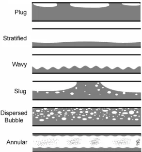
The common flow patterns for vertical upward flow, that is where both phases are flowing upwards, in a circular tube are illustrated in Fig. 2. As the quality, x, is gradually increased from
zero, the flow patterns obtained are:
Figure 2. Flow patterns in vertical upward flow in a tube.
Bubbly flow: the gas (or vapor) bubbles are of approximately uniform size.
Slug flow: the gas flows as large bullet-shaped bubbles (there are also some small gas bubbles distributed throughout the liquid). This flow pattern sometimes is called Plug flow.
Churn flow: highly unstable flow of an oscillatory nature; the liquid near the tube wall continually pulses up and down.
Annular flow: the liquid travels partly as an annular film on the walls of the tube and partly as small drops distributed in the gas which flows in the center of the tube.
Wispy-Annular flow: as the liquid flow rate is increased in annular flow, the concentration of drops in the gas core increases; ultimately, droplet coalescence in the core leads to large lumps or streaks (wisp) of liquid in the gas core. This flow pattern is
characteristic of flows with high mass flux and was proposed by Hewitt (1982).
In addition, the word ‘Froth’ is sometimes used to describe a very finely divided and turbulent bubbly flow approaching an emulsion, while on other occasions it is used to describe churn flow (Chisholm, 1973).
Horizontal and Slightly Upward Inclined Flow Patterns
Predictions of flow patterns for horizontal flow is a more difficult problem than for vertical flow. For horizontal flow, the phases tend to separate due to differences in density, causing a form of stratified flow to be very common. This makes the heavier (liquid) phase tend to accumulate at the bottom of the pipe. When the flow occurs in a pipe inclined at some angle other than vertical or horizontal, the flow patterns take other forms. In these situations, a form of slug flow is very common. The effect of gravity on the liquid precludes stratification. The common flow patterns for horizontal and slightly upward inclined flows in a round tube are illustrated in Fig. 3. Flow patterns that appear here are more complex than those in vertical flow because the gravitational force acts normal to the direction of the flow rather than parallel to it, as was the case for the vertical flow, and this results in the asymmetry of the flow. As the quality, x, is gradually increased from zero, the
flow patterns obtained are:
Figure 3. Flow patterns in horizontal and slightly upward inclined flow in a tube.
Plug flow: the individual small gas bubbles have coalesced to produce long plugs. In the literature sometimes the flow pattern observed at very low flow quality, prior to the plug flow, is referred to as Bubbly flow. In this situation the gas bubbles tend to flow along the top of the tube.
Stratified flow: the gas-liquid interface is smooth. Note that this flow pattern does not usually occur; the interface is almost always wavy as in wavy flow.
Wavy flow: the wave amplitude increases as the gas velocity increases.
Slug flow: the wave amplitude is so large that the wave touches the top of the tube.
Annular flow: similar to vertical annular flow except that the liquid film is much thicker at the bottom of the tube than at the top.
The term Intermittent flow is also used in the literature to refer to the presence of plug and slug flows together. Many researchers define other flow patterns, and nearly a hundred different names have been used. Many of these are merely alternative names, while others delineate minor differences in the main flow patterns. The number of flow patterns shown in Figs. 2 and 3 probably represent the minimum which can sensibly be defined. Further general details can be found in Hewitt (1982).
Flow Pattern Determination
As suggested earlier it is important in the analysis of the two-phase flow systems to classify the flow into a number of ‘flow patterns’ or ‘flow regimes’. This helps in obtaining a qualitative understanding of the flow and will also lead to better prediction methods for the various two-phase flow parameters. A detailed discussion of flow pattern determination is given by Hewitt (1978).
The most straightforward way of determining the flow pattern is to observe the flow in a transparent tube, or through a transparent window through the tube wall. However, the phenomena often occur at too high a speed for clear observation and high-speed photography or related techniques must be used. Unfortunately, even with high speed photography, it is not always possible to observe the structure of the two-phase flow clearly, due to the complex light refraction paths within the medium. In these cases X-ray photography can be very useful.
The unreliability of photographic methods in certain applications has led some researchers to seek other techniques for flow pattern categorization. The most popular of these is to insert a needle facing directly into the flow and to measure the current from the tip of this needle, through the two-phase flow, to the wall of the tube. The current is displayed on an oscilloscope and the type of response is considered to be representative of the flow pattern. For example, if no contacts are made between the needle and the wall, one may assume a continuous gas core and, thus, annular flow. High frequency interruptions of the current indicate bubble flow, and so on. Although the visual and contact methods agree reasonably well, where the flow pattern is clearly defined, discrepancies arise in the transition regions. The X-ray photography method is, therefore more reliable in examining these regions.
Four other techniques that have shown some promise in the determination of flow pattern will be briefly introduced here, refer to Hewitt (1978) for additional details: (a) Electro-chemical measurement of wall shear stress - in heated two-phase flow, the wall shear stress measurements can be related to flow pattern; (b) X-ray fluctuations – this method uses the instantaneous measurement of void fraction, using X-ray absorption, as a means of defining the flow pattern; (c) Analysis of pressure fluctuations – measurements of fluctuating pressure have been used to identify flow pattern; and (d) Multi-beam X-ray method – this method has been effective in determination of flow patterns in horizontal tubes, in this case the flow is asymmetric and the distribution of void fraction can give important clues about the flow pattern.
Due to multitude of flow patterns and the various interpretations accorded to them by different investigators, the general state of knowledge on flow patterns is unsatisfactory and no uniform procedure exists at present for describing and classifying them.
Flow Pattern Maps
Flow pattern map is an attempt, on a two-dimensional graph, to separate the space into areas corresponding to the various flow patterns. Simple flow pattern maps use the same axes for all flow
patterns and transitions. Complex flow pattern maps use different axes for different transition regions. The following are examples of some common flow pattern maps in the literature.
Vertical Flow Pattern Maps
The commonly recommended map for gas-liquid upward vertical flow is the Hewitt and Roberts (1969) map. On this map (Fig. 4), each coordinate is the superficial momentum fluxes for the respective phases. The Hewitt and Roberts (1969) map works reasonably well for air-water and steam-water systems. However, the transitions between the neighbor flow regimes appear as lines, which actually occur over a range of given coordinate terms. Thus, the transitions should be rather interpreted as broad bands than as lines (Whalley, 1996; Kim, 2000).
Figure 4. Hewitt and Roberts (1969) map for vertical flow.
Horizontal Flow Pattern Maps
Taitel and Dulker (1976) introduced theoretical models for determining transition boundaries of five flow regimes in horizontal and near horizontal two-phase gas-liquid flow. The theory was developed in dimensionless form, and the flow regime boundaries were introduced as a function of four dimensionless parameters. One is the Martinelli parameter, X, and the rest of them are defined
as follows:
2 1
cos ) (
) (
− =
θ ρ
ρ g
dz dp T
G L
SL
(35)
θ ρ
ρ ρ
cos
g D
u
F SG
G L
G −
= (36)
2 1 2 1
SL L
SL
Re F v
u D F
K =
= (37)
Figure 5. Taitel and Dulker (1976) map for horizontal flow.
Weisman et al. (1979) studied the effects of fluid properties (liquid viscosity, liquid density, interfacial tension, and gas density) and pipe diameters [1.27cm to 5.08cm (0.5in to 2in) I.D.] on two-phase flow patterns in horizontal pipes. The flow pattern data resulted in an overall flow pattern map (see Fig. 6) in terms of uSG and uSL, and dimensionless correlations were introduced in order to predict the transition boundaries.
Figure 6. Weisman et al. (1979) map for horizontal flow.
Spedding and Nguyen (1980) provided flow regime maps for conditions from vertically downward to vertically upward flow based on air-water flow data. Among 11 flow pattern maps provided, the flow pattern map for horizontal flow shows four main flow patterns (stratified flow, bubble and slug flow, droplet flow and mixed flow) and further 13 flow pattern subdivisions of the main flow patterns (see Fig. 7).
Figure 7. Spedding and Nguyen (1980) map for horizontal flow.
Slightly Upward Inclined Flow Pattern Maps
Small tube inclination angles are common in industrial applications, such as pipelines on the sea bed or passing over hilly terrain. There are very few flow pattern data and flow pattern maps available in the literature for tubes with small angles of inclination. There are some data available for steeply inclined tubes. However, most of the available information is for vertical or horizontal tubes. The very limited available information on tubes with small angles of inclination shows that inclination angle in certain cases does influence the flow patterns. For example, the study of Barnea et al. (1980) showed that the boundary of the stratified–intermittent transition changed dramatically with small angles of inclination. In contrast, according to Hewitt (1982), the boundaries of the intermittent–dispersed-bubble and annular–intermittent transitions were not changed much with small angles of inclination. Later on in this paper we will present some of the results of our study for upward inclination angles of 2°, 5°, and 7°. Flow pattern maps for these small inclination angles are not available in the literature.
Measurement Techniques
In non-boiling heat transfer in two-phase flow in pipes there are three parameters of significance. These include pressure drop, void fraction, and heat transfer coefficient. In this section the types of methods employed for the measurement of these primary parameters will be briefly discussed, see Hewitt (1982) for further details.
Measurement of Pressure Drop
In two-phase flow, measurement of pressure drop presents special difficulties because of possible ambiguities of the content of the lines joining the tapping points to the measuring device. Another problem is that of pressure drop fluctuations, which tend to be quite large in two-phase systems. A further area of difficulty is that of making pressure drop measurements in heated systems, particularly systems that are Joule-heated. Among the most important techniques available for measuring pressure drop are:
(1) Pressure drop measurement using fluid/fluid manometers – to determine the pressure difference from the manometer difference, the density of the fluid in the tapping lines must be known. In practice, this means that the lines must be filled with either single-phase gas or single-phase liquid. Unfortunately, the content of the lines can become two-phase by a variety of mechanisms such as: changes in pressure drop, condensation or evaporation in the lines, or pressure fluctuations in the tube. Generally improved performance can be obtained by purging the lines continuously with liquid.
(2) Pressure drop measurement using subtraction of signals from two locally mounted pressure transducers – if a very rapid response is required, then this method is the only feasible technique to use. The most obvious problem with this method is that signals from two separate instruments are being measured and subtracted, and this obviously increases error. Special care has to be taken in calibrating the transducers and in ensuring that the outputs are properly converted to the required pressure drop.
Measurement of Void Fraction
In two-phase flow, void fraction measurement is important in the calculation of pressure gradients and is relevant to the calculation of the amount of liquid and gas present in a system. There are numerous methods that have been proposed for the measurement of void fractions. For practical purposes, there are four main types of void fraction measurement:
(1) Pipe-average measurements –the average void fraction is required over a full section of pipe. A convenient and practical method for obtaining pipe-average measurements is the use of quick-closing valves. In this method, valves (which can be quickly and simultaneously operated) are placed at the beginning and end of a section of pipe over which the void fraction is to be determined. At the appropriate moment, the valves are actuated and the liquid phase trapped in the pipe is drained and its volume measured. Since the pipe volume is known or can be estimated, the pipe-average void fraction can be found. The valves can be linked mechanically or they can be operated by hand. For high pressure systems, solenoid valves may be used.
(2) Cross-sectional average measurements – the average void fraction is sought over a given pipe cross section. This can be achieved by using traversable single-beam radiation absorption methods, multibeam radiation absorption techniques, or neutron-scattering techniques.
(3) Chordal-average void fraction measurements – the average void fraction is measured across the diameter of a pipe. This type of measurement is usually achieved by means of radiation absorption methods.
(4) Local void fraction measurements – in this case void fraction is measured at a particular position within the pipe using local optical or electrical void probes. Usually, this void fraction is a time average at a point.
Measurement of Heat Transfer Coefficient
The heat transfer coefficient (defined as the ratio of the heat flux from a surface to the difference between the surface temperature and a suitably defined fluid bulk temperature) is of great importance in two-phase flow systems. For non-boiling heat transfer in gas-liquid flow in pipes, the most accepted and practical method of heat transfer coefficient measurement is the use of direct electrical heating with external thermocouples. In this method, alternating or direct current is fed through low-resistance leads and current clamps to the test section, which, typically, is a stainless steel tube through which the current passes. The power generation in the tube is determined by the product of the measured current that passes through the tube and the voltage drop across the tube. The power may be distributed nominally uniform if the wall thickness is uniform, but nonuniform axial and circumferential flux distributions are possible through the use of variable wall thickness. Usually, the temperature is measured on the outside of the tube wall with a thermocouple; the thermocouple junction is electrically insulated from the tube wall, using an epoxy adhesive with high thermal conductivity and electrical resistivity. The local inside tube wall temperature and the local peripheral inside wall heat flux is then calculated from measurements of the outside wall temperature, the heat generation within the pipe wall, and the thermophysical properties of the pipe material (electrical resistivity and thermal conductivity). From the local inside wall temperature, the local peripheral inside wall heat flux, and the local bulk temperature, the local peripheral heat transfer coefficient can be calculated. An example of the application of this method is the finite-difference based interactive computer program developed by Ghajar and Zurigat (1991). A brief description of the finite-difference
formulation and the equations used in the program, and the program’s capabilities will be presented next.
Finite Difference Formulation
The numerical solution of the conduction equation with internal heat generation and variable thermal conductivity and electrical resistivity was based on the following assumptions (Ghajar and Zurigat, 1991):
1. Steady-state conditions exist.
2. Peripheral and radial wall conduction exists. 3. Axial conduction is negligible.
4. The electrical resistivity and thermal conductivity of the tube wall are functions of temperature.
Based on the above assumptions, the expressions for calculation of the local inside wall temperatures, heat flux, and local and average peripheral heat transfer coefficients are presented next.
Calculation of the Local Inside Wall Temperature and the Local Inside Wall Heat Flux
The heat balance on a segment of the tube wall at any particular station is given by (see Fig. 8)
Figure 8. Finite-difference grid arrangement (Ghajar and Zurigat, 1991).
4 3 2
1 q q q
q
qg = + + + (38)
From Fourier’s law of heat conduction in a given direction n, we know that
dn dT A k
q=− (39)
Now substituting Fourier's law and applying the finite-difference formulation for the radial (i) and peripheral (j) directions
in Eq. (38), we obtain:
r T T
N z r r k
k
q ij i j
TH i j i j i
∆ − ∆ ∆ + +
= − 2 ( 2) ( − )
2 )
( , 1, , 1,
1
π
(40)
TH i
j i j i j
i j i
N r
T T z r k k q
π 2
) (
) ( 2
)
( , , 1 , , 1
2
+
+ ∆ ∆ −
+
= (41)
r T T
N z r r k
k
q ij i j
TH i j i j i
∆ − ∆ ∆ − +
= + 2 ( 2) ( + )
2 )
( , 1, , 1,
3
π
(42)
TH i
j i j i j
i j i
N r
T T z r k k q
π 2
) (
) ( 2
)
( , , 1 , , 1
4
−
− ∆ ∆ −
+
The heat generated in the (i, j) elemental volume is given by:
R I
qg = 2 (44)
Substituting R=γl/A and A=(2πri/NTH)∆r into Eq. (44) gives: r N r z I q TH i g ∆ ∆ = ) 2 ( 2 π γ (45)
Substituting Eqs. (40) to (43) and (45) into Eq. (38) and solving for Ti+1,j gives:
∆ ∆ − + − ∆ + − − ∆ + − − ∆ ∆ + + − ∆ − = + − − + + − − + TH i j i j i j i j i i TH j i j i j i j i i TH j i j i j i j i TH i j i j i i TH j i j i N r r r k k T T r N r k k T T r N r k k T T N r r r k k r r N I T
T ( ) ( 2)
) ( 4 ) ( ) ( 4 ) ( ) ( ) 2 ( ) ( 2 , 1 , 1 , , 1 , , 1 , , , 1 , , 1 , , 1 , 2 , , 1 π π π π π γ (46)
Equation (46) was used to calculate the temperature of the interior nodes. In this equation, the thermal conductivity and electrical resistivity of each node's control volume were determined as a function of temperature from the following equations for 316 stainless steel (Ghajar and Zurigat, 1991).
T
k=7.27+0.0038 (47)
T 0213 . 0 67 . 27 + = γ (48)
where T is in °F, k is in Btu/hr-ft-°F, and γ is in µΩ-in. Once the local inside wall temperatures were calculated from Eq. (46), the local peripheral inside wall heat flux could be calculated from the heat balance equation [see Eq. (38)].
Calculation of the Local Peripheral and Local Average Heat Transfer Coefficients
From the local inside wall temperature, the local peripheral inside wall heat flux and the local bulk fluid temperature, the local peripheral heat transfer coefficient could be calculated as follows:
) (TW TB
q
h= ′′ − (49)
Note that, in this analysis, it was assumed that the bulk temperature increases linearly in the pipe from the inlet to the outlet according to the following equation:
L x T T T
TB= IN+( OUT − IN) (50)
The local average heat transfer coefficient at each station is calculated by the following equation:
( )
( )
[
W k B k]
k
k q T T
h = ′′ − (51)
where k is the index of a thermocouple station.
Overall Mean Heat Transfer Coefficient
The local average peripheral values for inside wall temperature, inside wall heat flux, and heat transfer coefficient were then obtained by averaging all the appropriate individual local peripheral values at each axial location. The large variation in the circumferential wall temperature distribution, which is typical for two-phase gas-liquid flow in vertical, horizontal and slightly inclined tubes, leads to different heat transfer coefficients depending on which circumferential wall temperature was selected for calculations. In two-phase flow, in order to overcome the unbalanced circumferential heat transfer coefficient, Eq. (52) is recommended for calculation of the overall mean two-phase heat transfer coefficient, hTP.
∑
= Nst k
k st
TP h
N
h 1 (52)
where Nstis the number of all thermocouple stations and k is the index of a thermocouple station.
Physical Properties of the Working Fluids
The computer program developed by Ghajar and Zurigat (1991) also calculates the pertinent fluid flow and heat transfer dimensionless numbers. For this purpose the physical properties of the working fluids are needed. For example, for non-boiling two-phase heat transfer in air-water flow in pipes, the physical property correlations provided in Table 1 are recommended. Physical property expressions for other working fluids can easily be incorporated into the computer program.
Table 1. Physical properties of air and water, Vijay (1978).
Fluid Equation for the Physical Property
(T = Temperature in °F except where noted) Range of Validity & Accuracy
Air
ρ (lbm/ft3) = p/RT
where p is in lbf/ft2, T is in °R, and R = 53.34 ft⋅lbf/lbm⋅°R
cp (Btu/lbm⋅°F) = 7.540×10⁻⁶T + 0.2401
µ (lbm/ft⋅hr) = -2.637×10⁻⁸T 2 + 6.819×10⁻⁵T + 0.03936
k (Btu/hr⋅ft⋅°F) = -6.154×10⁻⁹T 2 + 2.591×10⁵T+ 0.01313
p≤150 psi
-10 ≤ T ≤ 242, 0.2 % -10 ≤ T ≤ 242, 0.1 % -10 ≤ T ≤ 242, 0.2 %
Water
ρ (lbm/ft3) = (2.101×10⁻⁸T 2 – 1.303×10⁻⁶T + 0.01602)-1
cp (Btu/lbm⋅°F) = 1.337×10⁻⁶T 2 – 3.374×10⁻⁴T + 1.018 µ (lbm/ft⋅hr) = (1.207×10
-5
T 2 + 3.863×10⁻³T + 0.0946)-1
k (Btu/hr⋅ft⋅°F) = 4.722×10⁻⁴T+ 0.3149
Data Reduction
The computer program developed by Ghajar and Zurigat’s (1991) can also be used to reduce the experimental data obtained for non-boiling two-phase heat transfer in gas-liquid flow in pipes under uniform wall heat flux boundary conditions. As will be discussed in the next section, at Oklahoma State University’s Heat Transfer Laboratory, we have used this computer program to reduce our air-water non-boiling heat transfer experimental data. The data reduction portion of the program reads a raw data file for a test run and then proceeds to perform all the required calculations. The results of the data reduction are saved in an output file for that particular test run. Figure 9 shows the data reduction results for the
case of air-water slug flow in a uniformly heated horizontal pipe. As can be seen from Fig. 9, the output file has four distinct sections to it. The first part of the output provides a detailed summary of the specifics of a test run, the second part gives the details of the pertinent heat transfer and flow information at each thermocouple station, the third part provides additional details at each thermocouple station that is more suited for the development of heat transfer correlations, and finally the forth and the last part of the output gives information about the flow parameters that are typically used in determination of flow patterns through established flow maps.
=============================================== RUN NUMBER 4649
FLOW PATTERN: S
Air-Water Two-phase Heat Transfer Test Date: 01-04-2004 SI UNIT VERSION
=============================================== LIQUID VOLUMETRIC FLOW RATE : 1.351 [m^3/hr] GAS VOLUMETRIC FLOW RATE : 3.086 [m^3/hr] LIQUID MASS FLOW RATE : 1351.36 [kg/hr] GAS MASS FLOW RATE : 4.777 [kg/hr] LIQUID V_SL : 0.615 [m/s] GAS V_SG : 1.406 [m/s] ROOM TEMPERATURE : 14.48 [C] INLET TEMPERATURE : 13.36 [C] OUTLET TEMPERATURE : 14.32 [C] AVG REFERENCE GAGE PRESSURE : 26169.74 [Pa] AVG LIQUID RE_SL : 14670 AVG GAS RE_SG : 3399 AVG LIQUID PR : 8.302 AVG GAS PR : 0.712
AVG LIQUID DENSITY : 1000.3 [kg/m^3] AVG GAS DENSITY : 1.548 [kg/m^3] AVG LIQUID SPECIFIC HEAT : 4.200 [kJ/kg-K] AVG GAS SPECIFIC HEAT : 1.007 [kJ/kg-K] AVG LIQUID VISCOSITY : 116.92e-05 [Pa-s] AVG GAS VISCOSITY : 17.84e-06 [Pa-s] AVG LIQUID CONDUCTIVITY : 0.592 [W/m-K] AVG GAS CONDUCTIVITY : 25.24e-03 [W/m-K] CURRENT TO TUBE : 460.51 [A] VOLTAGE DROP IN TUBE : 3.56 [V] AVG HEAT FLUX : 7089.12 [W/m^2] Q = AMP*VOLT : 1639.27 [W] Q = M*C*(T2 -T1) : 1512.20 [W] HEAT BALANCE ERROR : 7.75 [%] OUTSIDE SURFACE TEMPERATURE OF TUBE [C]
1 2 3 4 5 6 7 8 9 10 1 16.39 16.94 17.01 17.13 17.19 17.40 17.46 17.70 17.60 17.85 2 16.06 16.22 16.48 16.61 16.88 17.06 17.19 17.16 17.39 17.45 3 15.70 15.90 16.00 16.12 16.38 16.35 16.59 16.49 16.58 16.61 4 16.04 16.37 16.32 16.70 16.82 17.04 17.23 17.23 17.28 17.40 INSIDE SURFACE TEMPERATURES [C]
1 2 3 4 5 6 7 8 9 10 1 15.70 16.26 16.33 16.45 16.51 16.72 16.77 17.02 16.92 17.17 2 15.37 15.53 15.79 15.92 16.20 16.38 16.51 16.47 16.70 16.76 3 15.01 15.20 15.30 15.42 15.68 15.65 15.89 15.79 15.88 15.90 4 15.35 15.68 15.63 16.01 16.13 16.35 16.54 16.54 16.59 16.71 SUPERFICIAL REYNOLDS NUMBER OF GAS AT THE INSIDE TUBE WALL
1 2 3 4 5 6 7 8 9 10 1 3382 3377 3376 3375 3375 3373 3372 3370 3371 3369 2 3385 3384 3381 3380 3378 3376 3375 3375 3373 3372 3 3388 3387 3386 3385 3382 3383 3380 3381 3380 3380 4 3385 3382 3383 3379 3378 3376 3374 3374 3374 3373 SUPERFICAL REYNOLDS NUMBER OF LIQUID AT THE INSIDE TUBE WALL
1 2 3 4 5 6 7 8 9 10 1 15406 15625 15655 15703 15725 15810 15832 15930 15890 15991 2 15274 15337 15441 15492 15601 15673 15725 15712 15803 15826 3 15130 15206 15245 15292 15397 15383 15480 15440 15474 15485 4 15265 15396 15376 15527 15574 15663 15739 15738 15759 15806 INSIDE SURFACE HEAT FLUXES [W/m^2]
1 2 3 4 5 6 7 8 9 10 1 6639 6598 6603 6623 6645 6644 6661 6623 6658 6635 2 6686 6719 6695 6695 6681 6669 6674 6688 6656 6669 3 6739 6750 6752 6772 6764 6799 6788 6801 6808 6818 4 6689 6697 6718 6683 6691 6673 6668 6679 6672 6676 PERIPHERAL HEAT TRANSFER COEFFICIENT [W/m^2-K]
1 2 3 4 5 6 7 8 9 10 1 2911 2408 2424 2409 2448 2346 2383 2246 2415 2276 2 3433 3334 3064 3014 2780 2677 2639 2781 2622 2662 3 4251 4005 3990 3943 3577 3857 3547 3951 3967 4130 4 3471 3094 3325 2895 2865 2705 2599 2705 2746 2721
=============================================== RUN NUMBER 4649 continued
FLOW PATTERN: S
===============================================
ST MU_L[E-5 Pa-s] MU_G[E-6 Pa-s] CP[kJ/kg-K] K[W/m-K] RHO[kg/m^3] Bulk Wall Bulk Wall Lqd Gas Lqd Gas(E-3) Lqd Gas 1 118.23 112.34 17.82 17.91 4.200 1.007 0.591 25.21 1000.3 1.550 2 117.94 111.45 17.82 17.93 4.200 1.007 0.591 25.22 1000.3 1.550 3 117.65 111.17 17.83 17.93 4.200 1.007 0.591 25.22 1000.3 1.549 4 117.36 110.64 17.83 17.94 4.200 1.007 0.591 25.23 1000.3 1.549 5 117.07 110.14 17.84 17.95 4.200 1.007 0.591 25.24 1000.3 1.548 6 116.78 109.73 17.84 17.96 4.200 1.007 0.592 25.25 1000.3 1.548 7 116.49 109.30 17.85 17.96 4.200 1.007 0.592 25.25 1000.3 1.547 8 116.21 109.22 17.85 17.97 4.200 1.007 0.592 25.26 1000.3 1.547 9 115.93 109.04 17.85 17.97 4.199 1.007 0.592 25.27 1000.2 1.546 10 115.64 108.72 17.86 17.97 4.199 1.007 0.592 25.27 1000.2 1.546 ST X/D RESL RESG PRL PRG MUB/W(L) MUB/W(G) HT/HB HFLUX TB[C] TW[C] HCOEFF NU_L 1 6.38 14508 3403 8.40 0.712 1.052 0.995 0.685 6688 13.42 15.36 3456.3 162.98 2 15.50 14544 3402 8.38 0.712 1.058 0.994 0.601 6691 13.52 15.67 3110.4 146.64 3 24.61 14580 3401 8.36 0.712 1.058 0.994 0.608 6692 13.61 15.76 3104.9 146.34 4 33.73 14616 3400 8.34 0.712 1.061 0.994 0.611 6693 13.70 15.95 2976.0 140.23 5 42.84 14652 3400 8.31 0.712 1.063 0.994 0.684 6695 13.79 16.13 2866.4 135.04 6 51.96 14688 3399 8.29 0.712 1.064 0.994 0.608 6696 13.89 16.27 2803.9 132.06 7 61.08 14724 3398 8.27 0.712 1.066 0.993 0.672 6698 13.98 16.43 2732.8 128.69 8 70.19 14760 3397 8.25 0.712 1.064 0.994 0.569 6698 14.07 16.46 2807.1 132.16 9 79.31 14797 3396 8.22 0.712 1.063 0.994 0.609 6699 14.16 16.52 2838.1 133.58 10 88.42 14833 3395 8.20 0.712 1.064 0.994 0.551 6700 14.25 16.63 2813.5 132.39 ===============================================
RUN NUMBER 4649 continued FLOW PATTERN: S
QUANTITIES OF MAIN PARAMETERS
=============================================== INCLINATION ANGLE : 2.000 [DEG] TOTAL MASS FLUX(Gt): 617.775 [kg/m^2-s] QUALITY(x) : 0.004
SLIP RATIO(K) : 1.809 VOID FRACTION(alpa): 0.558 V_SL : 0.615 [m/s] V_SG : 1.406 [m/s] RE_SL : 14670 RE_SG : 3399 RE_TP : 18069 X(Taitel & Dukler) : 9.614 T(Taitel & Dukler) : 0.137 Y(Taitel & Dukler) : 172.059 F(Taitel & Dukler) : 0.106 K(Taitel & Dukler) : 12.828 X (Breber) : 9.614 j*g(Breber) : 0.106
Figure 9. (Continued).
Oklahoma State University’s Heat Transfer Laboratory Research in Two-Phase Flow
In the next several sections we present the results of our extensive literature search, a detailed development of our proposed heat transfer correlation and its application to experimental data in vertical and horizontal pipes, a detailed description of our experimental setup, our flow visualization results for different flow patterns, our experimental results for slug and annular flows in horizontal and inclined tubes, our proposed heat transfer correlation for these flow patterns and pipe orientations, and finally our future plans.
Comparison of Non-Boiling Two-Phase Heat Transfer Correlations with Experimental Data
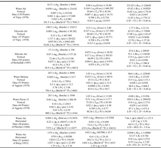
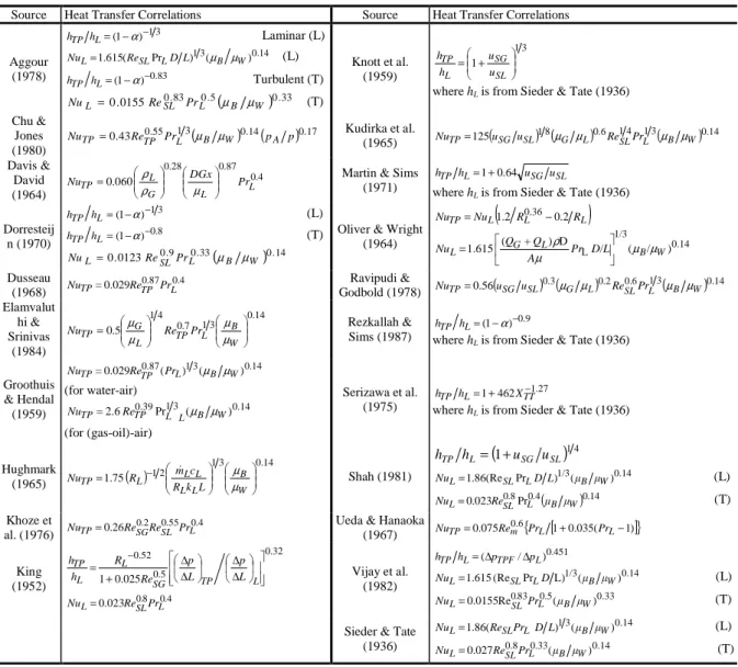
Numerous heat transfer correlations and experimental data for non-boiling forced convective heat transfer during gas-liquid two-phase flow in vertical and horizontal pipes have been published over the past 50 years. In a study published by Kim et al. (1999), a comprehensive literature search was carried out and a total of 38 two-phase flow heat transfer correlations were identified. The validity of these correlations and their ranges of applicability have been documented by the original authors. In most cases, the identified heat transfer correlations were based on a small set of experimental data with a limited range of variables and liquid-gas
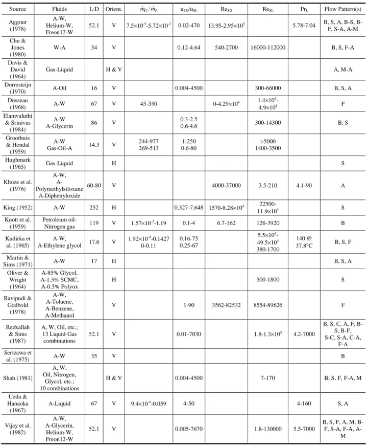
combinations. In order to assess the validity of those correlations, they were compared against seven extensive sets of two-phase flow non-boiling heat transfer experimental data available from the literature, for vertical and horizontal tubes and different flow patterns and fluids. For consistency, the validity of the identified heat transfer correlations were based on the comparison between the predicted and experimental two-phase heat transfer coefficients meeting the ±30% criterion. A total of 524 data points from the five available experimental studies (see Table 2) were used for these comparisons. The experimental data included five different liquid-gas combinations (water-air, glycerin-air, silicone-air, water-helium, water-Freon 12), and covered a wide range of variables, including liquid and gas flow rates and properties, flow patterns, pipe sizes, and pipe inclination. Five of these experimental data sets are concerned with a wide variety of flow patterns in vertical pipes and the other two data sets are for limited flow patterns (slug and annular) within horizontal pipes.
Table 2. Ranges of the experimental data used in the study of Kim et al. (1999).
Water-Air Vertical Data (139 Points)
of Vijay (1978)
16.71 ≤mL(lbm/hr) ≤ 8996 0.058 ≤m (lbm/hr) G ≤ 216.82
0.007 ≤ XTT≤ 433.04 0.061 ≤∆pTP (psi) ≤ 17.048
5.503 ≤ PrL≤ 6.982 101.5 ≤ hTP (Btu/hr⋅ft2⋅°F) ≤ 7042.3
0.06 ≤ uSL(ft/sec) ≤ 34.80 0.164 ≤ uSG(ft/sec) ≤ 460.202
59.64 ≤ Tm (°F) ≤ 83.94 0.007 ≤∆pTPF (psi) ≤ 16.74
0.708 ≤ PrG≤ 0.710 0.813 ≤µW/µB≤ 0.933
231.83 ≤ ReSL≤ 126630 43.42 ≤ ReSG≤ 163020 14.62 ≤ pm (psi) ≤ 74.44
0.033 ≤α≤ 0.997 11.03 ≤ NuTP≤ 776.12 L/D = 52.1, D = 0.46 in.
Glycerin-Air Vertical Data (57 Points) of Vijay (1978)
100.5 ≤mL(lbm/hr) ≤ 1242.5 0.085 ≤m (lbm/hr) G ≤ 99.302
0.15 ≤ XTT≤ 407.905 1.317 ≤∆pTP (psi) ≤ 20.022
6307.04 ≤ PrL≤ 6962.605 54.84 ≤ hTP (Btu/hr⋅ft2⋅°F) ≤ 159.91
0.31 ≤ uSL (ft/sec) ≤ 3.80 0.217 ≤ uSL (ft/sec) ≤ 117.303
80.40 ≤ Tm (°F) ≤ 82.59 1.07 ≤∆pTPF (psi) ≤ 19.771
0.708 ≤ PrG≤ 0.709 0.513 ≤µW/µB≤ 0.610
1.77 ≤ ReSL≤ 21.16 63.22 ≤ ReSG≤ 73698 17.08 ≤ pm (psi) ≤ 62.47
0.0521 ≤α≤ 0.9648 12.78 ≤ NuTP≤ 37.26 L/D = 52.1, D = 0.46 in.
Silicone-Air Vertical Data (162 points) of Rezkallah (1987)
17.3 ≤mL(lbm/hr) ≤ 196 0.07 ≤mG(lbm/hr) ≤ 157.26
72.46 ≤ TW (°F) ≤113.90 0.037 ≤∆pTP (psi) ≤ 9.767
61.0 ≤ PrL≤ 76.5 29.9 ≤ hTP (Btu/hr⋅ft2⋅°F) ≤ 683.0
0.072 ≤ uSL (ft/sec) ≤ 30.20 0.17 ≤ uSL (ft/sec) ≤ 363.63 66.09 ≤ TB (°F) ≤ 89.0 0.094 ≤∆pTPF (psi) ≤ 9.074
0.079 ≤ PrG≤ 0.710
47.0 ≤ ReSL≤ 20930 52.1 ≤ ReSG≤ 118160 13.9 ≤ pm (psi) ≤ 45.3 0.011 ≤α≤ 0.996 17.3 ≤ NuTP≤ 386.8 L/D = 52.1, D = 0.46 in.
Water-Helium Vertical Data (53 Points) of Aggour (1978)
267 ≤mL(lbm/hr) ≤ 8996 0.020 ≤m (lbm/hr) G ≤ 33.7
0.16 ≤ XTT≤ 769.6 0.3 ≤∆pTP (psi) ≤ 13.2
5.78 ≤ PrL≤ 7.04 794 ≤ hTP (Btu/hr⋅ft2⋅°F) ≤ 6061
1.03 ≤ uSL (ft/sec) ≤ 34.70 0.423 ≤ uSL (ft/sec) ≤ 483.6 67.4 ≤ Tm (°F) ≤ 82.0 0.01 ≤∆pTPF (psi) ≤ 12.5
0.6908 ≤ PrG≤ 0.691 83.9 ≤ TW (°F) ≤ 95.7
3841 ≤ ReSL≤ 125840 14.0 ≤ ReSG≤ 23159 15.5 ≤ pm (psi) ≤ 53.3
0.038 ≤α≤ 0.958 86.6 ≤ NuTP≤ 668.2 L/D = 52.1, D = 0.46 in
Water-Freon 12 Vertical Data (44 Points) of Aggour (1978)
267 ≤mL(lbm/hr) ≤ 3598 0.84 ≤m (lbm/hr) G ≤ 206.59
0.16 ≤ XTT≤ 226.5 0.04 ≤∆pTP (psi) ≤ 4.92
5.63 ≤ PrL≤ 6.29 800 ≤ hTP (Btu/hr⋅ft2⋅°F) ≤ 4344
1.03 ≤ uSL (ft/sec) ≤ 13.89 0.51 ≤ uSL (ft/sec) ≤ 117.7 75.26 ≤ TMIX (°F) ≤ 83.89 0.02 ≤∆pTPF (psi) ≤ 4.48
0.769 ≤ PrG≤ 0.77 90.36 ≤ TW (°F) ≤ 94.89
4190 ≤ ReSL≤ 51556 859.5 ≤ ReSG≤ 209430
15.8 ≤ pm (psi) ≤ 27.8 0.035 ≤α≤ 0.934 87.1 ≤ NuTP≤ 472.4 L/D = 52.1, D = 0.46 in
Water-Air Horizontal Data (48 points) of Pletcher (1966)
0.069 ≤mL(lbm/sec) ≤ 0.3876 0.22 ≤∆pa/L (lbf/ft3) ≤ 26.35
7.23 ≤φL≤ 68.0 7372 ≤ q'' (Btu/hr⋅ft2) ≤ 11077
0.03 ≤mG(lbm/sec) ≤ 0.2568 0.021 ≤ XTT≤ 0.490 73.6 ≤ TW (°F) ≤ 107.1 433 ≤ hTP (Btu/hr⋅ft2⋅°F) ≤ 1043.8
7.84 ≤∆p/L (lbf/ft3) ≤ 137.5
1.45 ≤φG≤ 3.54 64.9 ≤ Tm (°F) ≤ 99.4 L/D = 60.0, D = 1.0 in.
Water-Air Horizontal Data (21 points)
of King (1952)
1375 ≤mL(lbm/hr) ≤ 6410 1570 ≤ ReSG≤ 84200 136.8 ≤ Tm (°F) ≤ 144.85 1.027 ≤∆pTP (psi) ≤ 22.403
1.35 ≤ hTP / hL≤ 3.34
0.82 ≤mG(SCFM) ≤ 43.7 0.41 ≤ XTT≤ 29.10 184.3 ≤ TW (°F) ≤ 211.3 1462 ≤ hTP (Btu/hr⋅ft2⋅°F) ≤ 4415
1.35 ≤φL≤ 8.20
22500 ≤ ReSL≤ 119000 0.117 ≤ RL≤ 0.746 15.8 ≤ pm (psi) ≤ 55.0
0.33 ≤ uSG/uSL≤ 7.65 L/D =252, D = 0.737 in.
For the limited experimental data in horizontal pipes (see Table 2), the correlation of Shah (1981) was the only correlation that performed well in predicting the annular flow data of Pletcher (1966). However, the experimental data of King (1952) for slug flow in a horizontal pipe were predicted very well by five of the identified heat transfer correlations. Figure 10 shows how well the correlations of Chu and Jones (1980), King (1952), Kudirka et al. (1965), Martin and Sims (1971), and Ravipudi and Godbold (1978) predicted the data of King (1952).
1000 1000
Chu & Jones (1980) King (1952) Kudirka et al. (1965) Martin & Sims (1971) Ravipudi & Godbold (1978) 2000 3000 4000 5000 6000 2000
3000 4000 5000 6000
+30 %
-30 %
hT PCAL
(
B
tu
/h
r-ft
2-°
F
)
hTPEXP (Btu/hr-ft
2 -°F)
Figure 10. Comparison of selected correlations with King (1952) slug flow air-water experimental data in a horizontal pipe.
(1978) is recommended for this set of experimental data. For the silicone-air experimental data of Rezkallah (1987) in a vertical tube, a few of the correlations predicted the experimental data reasonably well. Again, considering the overall performance of the correlations for all flow patterns and the values of the mean and rms deviations, only three of the tested heat transfer correlations were recommended. These are the correlation of Rezkallah and Sims (1987) for bubbly, slug, churn, bubbly-slug, bubbly-froth, slug-churn, and churn-annular flow patterns; the correlation of Ravipudi and Godbold (1978) for churn, annular, bubbly-slug, slug-churn, churn-annular and froth-annular flow patterns; and the correlation of Shah (1981) for bubbly, froth, bubbly-froth, froth-annular, and annular-mist flow patterns. Figure 12 provides a comparison of the predictions of Shah (1981) correlation with the silicone-air experimental data of Rezkallah (1987). For the water-helium experimental data of Aggour (1978) in a vertical tube, several correlations predicted the experimental data fairly well. Considering not only the overall performance of the correlations for all flow patterns but also the values of the mean and rms deviations, three of the tested heat transfer correlations were recommended. These were the correlation of Chu and Jones (1980) for bubbly, froth, and bubbly-slug flow patterns; the correlation of Knott et al. (1959) for all of the main flow patterns (bubbly, slug, froth, and annular) and slug-annular transitional flow; and the correlation of Shah (1981) for bubbly, froth, and annular-mist flow patterns. Figures 13 and 14 show the comparison between the predictions of Chu and Jones (1980) and Shah (1981) correlations with the water-helium experimental data of Aggour (1978). With respect to the water-Freon 12 experimental data of Aggour (1978), several of the tested heat transfer correlations were capable of predicting the experimental data with good accuracy. Considering the overall performance of the correlations for all flow patterns and also the mean and rms deviations, three of the tested correlations demonstrated good accuracy in predicting all of the main flow patterns (bubbly, slug, froth, and annular) and slug-annular transitional flow. These were the correlation of Aggour (1978), the correlation of Martin and Sims (1971), and the correlation of Rezkallah and Sims (1987). Figure 15 shows the performance of the predictions of Martin and Sims (1971) correlation with the water-Freon 12 experimental data of Aggour (1978) in a vertical pipe.
hTP
EXP
(Btu/hr-ft2-°F)
100 1000 10000
hTP
C
A
L
(
B
tu
/h
r-ft
2-°
F
)
10 100 1000 10000
Bubble Slug Froth Annular Bubble-Froth Slug-Annular Froth-Annular Annular-Mist Laminar Slug Laminar Annular Laminar Slug-Annular Laminar Annular-Mist +30 %
-30 %
Figure 11. Comparison of Knott et al. (1959) correlation with Vijay (1978) air-water experimental data in a vertical pipe.
hTPEXP (Btu/hr-ft
2 -°F)
10 100 1000 10000
hTP
C
A
L
(
B
tu
/h
r-ft
2-°
F
)
1 10 100 1000
Bubble Slug Churn Annular Froth Bubbly-Slug Bubbly-Froth Slug-Churn Churn-Annular Froth-Annular Annular-Mist Laminar Slug Laminar Churn Laminar Annular Laminar Slug-Churn Laminar Churn-Annular Laminar Annular-Mist +30 %
-30 %
Figure 12. Comparison of Shah (1981) Correlation with Rezkallah (1987) Silicone-Air Experimental Data in a Vertical Pipe.
hTPEXP (Btu/hr-ft2
2-°F)
1000 10000
hTP
C
A
L
(
B
tu
/h
r-ft
2-°
F
)
1000 10000
Bubbly Slug Froth Annular Bubbly-Slug Bubbly-Froth Slug-Annular Annular-Mist -30 %
+30 %
Figure 13. Comparison of Chu and Jones (1980) correlation with Aggour (1978) water-helium experimental data in a vertical pipe.
hTPEXP (Btu/hr-ft
2-°F)
1000 10000
hTP
C
A
L
(B
tu
/h
r-ft
2-°
F
)
1000 10000
Bubbly Slug Froth Annular Bubbly-Slug Bubbly-Froth Slug-Annular Annular-Mist -30 %
+30 %
Figure 14. Comparison of Shah (1981) correlation with Aggour (1978) water-helium experimental data in a vertical pipe.
hTPEXP (Btu/hr-ft
2-°F)
1000 10000
hT PCAL
(
B
tu
/h
r-ft
2-°
F
)
1000 10000
Bubbly Slug Froth Annular Bubbly-Slug Bubbly-Froth Slug-Annular -30 %
+30 %