Pesqui. Oper. vol.36 número1

doi: 10.1590/0101-7438.2016.036.01.0113

A HYBRID HEURISTIC ALGORITHM FOR THE CLUSTERED TRAVELING SALESMAN PROBLEM

M´ario Mestria

Received July 11, 2015 / Accepted March 21, 2016

ABSTRACT.This paper proposes a hybrid heuristic algorithm, based on the metaheuristics Greedy Ran-domized Adaptive Search Procedure, Iterated Local Search and Variable Neighborhood Descent, to solve the Clustered Traveling Salesman Problem (CTSP). Hybrid Heuristic algorithm uses several variable neigh-borhood structures combining the intensification (using local search operators) and diversification (con-structive heuristic and perturbation routine). In the CTSP, the vertices are partitioned into clusters and all vertices of each cluster have to be visited contiguously. The CTSP isN P_{-hard since it includes the}

well-known Traveling Salesman Problem (TSP) as a special case. Our hybrid heuristic is compared with three heuristics from the literature and an exact method. Computational experiments are reported for differ-ent classes of instances. Experimdiffer-ental results show that the proposed hybrid heuristic obtains competitive results within reasonable computational time.

Keywords: Combinatorial Problems, Clustered Traveling Salesman Problem, Hybrid Heuristic, GRASP, Iterated Local Search, Variable Neighborhood Structures.

1 INTRODUCTION

The Clustered Traveling Salesman Problem (CTSP) can be defined as follows. LetG= (V, E) be a symmetric complete graph with vertex setV={v1,v2, . . . , vn}and edge setE={(vi,vj) : vi,vj ∈ V,i = j }. The vertex set V is partitioned into disjoint clustersV1,V2, . . . ,Vm and each edge (vi,vj)∈ E is associated with a non-negative costci j. The objective of the CTSP is to find a minimum cost Hamiltonian tour onG, where all vertices of each cluster must be visited consecutively. Note that when there is only a subsetVi =V the CTSP becomes a Trav-eling Salesman Problem (TSP). Therefore, the CTSP isN P_{-hard since it includes the TSP as} a special case.

CTSP applications arise in automated warehouse routing Chisman [6], emergency vehicle dis-patching Weintraub, Aboud, Fernandez, Laporte & Ramirez [42], production planning Lokin

[27], computer disks defragmentation, manufacturing, vehicle routing Laporte & Palekar [24], commercial transactions with supermarkets and shops and grocery suppliers Ghaziri & Osman [16]. Heuristic techniques are widely used to solve many TSP variants Dong, Guo & Tickle [9], Escario, Jimenez & Giron-Sierra [10], and Nagata & Soler [35]. There are also heuristic procedures based on different approaches Fioruci, Toledo & Nascimento [13], Subramanian & Battarra [40], L´etocart, Plateau & Plateau [26], Mart´ınez, Alvarez-Valdes & Parre˜no [32], and Vidal, Battarra, Subramanian & Erdogan [41] to solve different variants of combinatorial opti-mization problems.

As pointed out in Caserta & Voß [5], a line of research in the metaheuristic field is concerned with the design of hybrid algorithms, where the term hybrid can indicate either the combination of different metaheuristics or the intertwined usage of metaheuristic features with mathematical programming techniques.

In L´opez-Ib´a˜nez, Mascia, Marmion & St¨utzle [28], the authors discuss a template for single-solution hybrid metaheuristics is based on Iterated Local Search (ILS). The flexibility is given by generalizing the components of ILS (perturbation, local search and acceptance criterion) in order to incorporate components from other metaheuristics.

In this context we propose a hybrid heuristic algorithm for the CTSP that is based on the meta-heuristics Greedy Randomized Adaptive Search Procedure (GRASP) Feo & Resende [11], ILS Lourenc¸o, Martin & St¨utzle [29], and Variable Neighborhood Descent (VND) Hansen & Mlade-novi´c [19]. To the best of our knowledge, this is the first time ILS has been applied to solve the CTSP. State-of-the-art solutions were found for many problems using this metaheuristic St¨utzle [39] and Lourenc¸o, Martin & St¨utzle [30]. The developed hybrid heuristic approach extends the basic GRASP structure by embedding ILS components, which in turn, makes use of a Vari-able Neighborhood Descent (VND) Hansen & Mladenovi´c [20] based procedure in the local search phase.

The remainder of the paper is organized as follows. Section 2 provides a brief review of some works related to the CTSP. Section 3 presents a mathematical formulation of CTSP. Section 4 describes the proposed hybrid heuristic for the CTSP. Computational results are given in Section 5 and conclusions are presented in Section 6.

2 RELATED WORK

adding a large constantM to the cost of each inter-cluster edge. A branch-and-bound algorithm was used to solve the problem.

Severalα-approximation algorithms were developed for the CTSP Anily, Bramel & Hertz [1], Arkin, Hassin & Klein [3], Gendreau, Laporte & Potvin [14], Gendreau, Laporte & Hertz [15], and Guttmann-Beck, Hassin, Khuller & Raghavachari [18]. These algorithms extend those de-veloped for the TSP Christofides [7] and Hoogeveen [21] and provide solutions for the CTSP within a given approximation factor. Different values for such factors were found in the litera-ture, namely: 5/3 Anily, Bramel & Hertz [1], 3.5 Arkin, Hassin & Klein [3], 2 Gendreau, Laporte & Potvin [14], and 3/2 Gendreau, Laporte & Hertz [15].

It is worth mentioning that theα-approximation algorithms require as input either the starting

si and ending ti vertices in each cluster Vi or a prespecified order of visiting the clusters in the tour, i.e., V1,V2, . . . ,Vm, withVi < Vj, j = i +1, fori = 1,2, . . . ,m−1. Note that these algorithms solve the inter-cluster and intra-cluster problems independently. One drawback of theseα-approximation algorithms is the fact that it does not allow the construction of cycles when the order of visiting the clusters is not givena priori.

In Guttmann-Beck, Hassin, Khuller & Raghavachari [18] someα-approximation algorithms with bounded performance ratios were presented for four CTSP variants. In the first one, a (21/11)-approximation algorithm was proposed for the case in which the starting and ending vertices of each cluster are specified. In the second one, a (9/5)-approximation algorithm was suggested for the variant where for each cluster the two end vertices are given, but with freedom of choos-ing the startchoos-ing and endchoos-ing vertices. The third approximation scheme consists of a (37/14)-approximation algorithm for the case where the starting vertex of each cluster is given. In the last one, a (11/4)-approximation algorithm was devised for the case where no specific starting and ending vertices are provided. More recently, in Bao & Liu [4], a new approximation algo-rithm with a factor of 13/6 was proposed for the CTSP, also for the case where no starting and ending vertices are specified.

A heuristic algorithm that combines the concepts of Tabu Search and Evolutionary Algorithms was proposed in Laporte, Potvin & Quilleret [25] to solve a particular case of the CTSP in which the visiting order within the clusters is prespecified. It was verified that the developed heuristic outperformed the Genetic Algorithm (GA) described in Potvin & Guertin [36], which exploits order-based crossover operators and local search heuristics. The CTSP with a prespecified vis-iting order within the clusters was also considered in Gendreau, Laporte & Potvin [14]. An approximation algorithm with guaranteed performance ratio and two methods with satisfactory empirical performance were developed. Three algorithms were compared with a lower bound.

A GA for the CTSP which finds inter-cluster paths and then intra-cluster paths was developed in Potvin & Guertin [37]. Comparisons were performed with the heuristic proposed in Gendreau, Laporte & Potvin [14] and with lower bounds obtained using the procedure suggested in Jon-gens & Volgenant [23]. This GA solved problems with up to 500 vertices and with 4 and 10 clusters. A Two-Level Genetic Algorithm (TLGA) was proposed for the CTSP in Ding, Cheng & He [8]. In the lower level, the algorithm finds Hamiltonian cycles in each cluster, whereas in the higher level, it randomly chooses an edge to be deleted on the cycle in each cluster and simultaneously determines routing among clusters. Computational results demonstrated that the TLGA outperformed the classical GA developed by the authors Ding, Cheng & He [8].

Several GRASP based heuristics for the CTSP were recently proposed in Mestria, Ochi & Martins [33]. One heuristic corresponds to the traditional GRASP while another five include alternative Path Relinking (Glover, Laguna & Mart´ı [17]) procedures. The computational re-sults showed that the proposed heuristics outperformed the GA presented in Ding, Cheng & He [8]. Two particular versions, GPR1R2 and GPR4, had the best performance among the different methods put forward by the authors. We compare the results obtained by our hybrid heuristic with those found by these two approaches and also with the traditional GRASP.

3 A MATHEMATICAL FORMULATION OF CTSP

A mathematical formulation of CTSP using integer programming is described in Chisman [6], Miller, Tucker & Zemlin [34]. The salesman leaves an origin cityv1, without loss of generality,

and returns tov1. The costci j represents the distance between cityvi and cityvj. The salesman proceeds from cityvi to cityvjif and only ifxi j=1.

The mathematical formulation is as follows:

Minimizez= n

i=1 n

j=1

ci jxi j (1)

subject to

n

j=1

xi j =1, ∀i ∈V (2)

n

i=1

xi j =1, ∀j ∈V (3)

ui−uj +(n−1)xi j ≤(n−2), 2≤i= j ≤n (4)

i∈Vk

j∈Vk

xi j =|Vk| −1, ∀Vk ⊂V,|Vk|≥1,k=1, . . . ,m (5)

ui ≥0 2≤i ≤n (6)

xi j ∈ {0,1} ∀i,j ∈V (7)

not begin and end at cityv1and tours that visit more than(n−1)cities. Constraints (5) state that

a Hamiltonian path of length|Vk| −1 must go through the|Vk|points of clusterk. Constraints (6) and (7) define the domain of variables.

9

11

10

8

5

V

1

V

6

1

4

3

2

7

V

V

Figure 1– A feasible solution for an example of an instance of the CTSP.

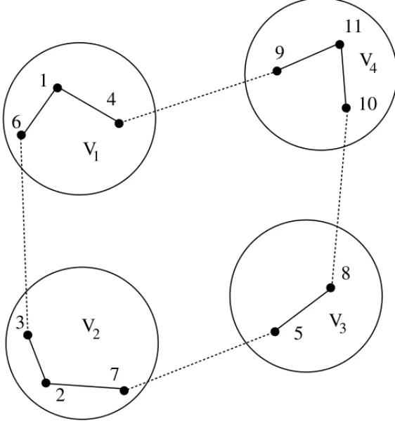
The Figure 1 shows a feasible solution for an example of an instance of the CTSP composed of four clusters (V1,V2,V3, andV4) and 11 vertices, whereV1={1, 4, 6},V2={2, 3, 7},V3={5, 8}, andV4={9, 10, 11}. The dotted line edge between the vertices 4 and 9 show a connection inter-cluster and the full line edge between the vertices 9 and 11 a intra-cluster connection. Note that the vertices of each cluster are visited contiguously.

4 THE PROPOSED HYBRID HEURISTIC

Algorithm 1Pseudocode of the HHGILS algorithm.

1: i ter pr ob←1;

2: initializealphas( );{initialize the probability distribution of the alphas}

3: for i=1 tomaxext do

4: S0←ConstructiveHeuristic(); 5: S←VND(S0);

6: for i=1 tomaxi nt do 7: S′←Pert(S); 8: S′′←VND(S′);

9: S←AccepCrit(S,S′′,S∗);

10: ifSis better thanS∗then

11: S∗←S;

12: end if 13: end for

14: ifi ter pr ob=max pr obthen

15: updatealphas( );{update the probability distribution of the alphas}

16: i ter pr ob←0;

17: end if

18: i ter pr ob++;

19: end for 20: return S∗;

Other three important parameters of the algorithm are: maxext,maxint andmax prob. They correspond, respectively, to the maximum number of restarts of the method, ILS iterations, and restarts to update the probability distribution ofα.

The value ofmaxintis typically larger thanmax probbecause more computational effort is usu-ally required to improve an initial solution than to improve another one that has been slightly modified (perturbed) from a local optimal solution. Restarting the method from a different ini-tial solution and perturbing local optimal solutions are both promising ways of diversifying the search, especially when put together. Since perturbations may lead to cycles, we build new so-lutions so as to avoid this kind of cycling. Thus at each external iteration a solution is built. For each of themaxext iterations (step 3 to step 19), a solution is generated by a constructive procedure based on GRASP and, in step 5, a local search is performed by means of a VND pro-cedure. For each of themaxint iterations (step 6 to step 13), a perturbation is applied in step 7 and a local search is performed again using VND (step 8). In steps 9-11, the incumbent solution is updated.

in choosing the solution which presents the minimum cost among the three solutionsS,S′′ and

S∗. In step 15, the probability distribution of theαvalues is updated using a reactive strategy. Finally, in step 20 the best solution is returned.

The constructive heuristic extends the well-known Nearest Insertion heuristic by introducing concepts of GRASP. At each iteration of the constructive heuristic, a Restricted Candidate List (RCL) is built using a parameterα to restrict the size of the list of candidates to be inserted in the partial solution. Theα values are defined using areactive strategy, leading to a better performance when compared with fixed values. The reactive strategy usually helps generating better quality solutions, also avoiding parameter tuning (Festa & Resende [12]). The reactive strategy is presented as follows. Let = {α1, . . . , αm}be the finite set ofmpossible values forαand let pi be the corresponding probability of selectingαi,i =1, . . . ,m. Initially,pi is uniformly distributed:

pi=1/m, i =1, . . . ,m. (8)

AfterK iterations, the pi values are reevaluated as follows. Let f∗ be the best cost solution found in K previous iterations and let fi be the average cost solutions obtained using α = αi,i =1, . . . ,mduringK iterations. The probabilities are updated afterK iterations according to:

pi =qi/ m

j=1

qj, i=1, . . . ,m. (9)

whereqi = f∗/fi.

Algorithm 2Pseudocode of the nearest insertion heuristic.

1: Select three verticesvl,vl+1andvl+2; 2: S← {vl,vl+1,vl+2};

3: Initialize the candidate setC←V\{vl,vl+1,vl+2}; 4: whileC= ∅do

5: Find theknearest vertices ofCwith respect to the vertices of the constructed tour (solution S) and evaluate the incremental costsc(vk)forvk ∈C;

6: cmin←mi n{c(vk)/vk∈C}; 7: cmax←max{c(vk)/vk∈C};

8: RC L← {vk∈C/c(vk)≤cmin+α∗(cmax−cmin)}; 9: Select an elementvkfrom theRC Lat random;

10: S ←S ∪{vk};{connectvk to the vertices (vi andvi+1) of the tour with minimum cost (price)

p(vk)={pi,k+pk,i+1-pi,i+1}and update the tour} 11: Update the candidate setC←C\{vk};

12: end while 13: return S

The pseudocode of the constructive heuristic is presented in Algorithm 2. In step 1, the vertexvl is randomly selected and the two nearest neighborhood vertices from the same cluster asvl(vl+1

Thecandidate set Cis initialized in step 3. In step 5, theknearest vertices ofC, with respect to the vertices already in the partial tour, are determined and the incremental costs c(vk)are evaluated. Only feasible insertions are considered, meaning that the vertices chosen belong to the same cluster of existing vertices in the partial solution. Note that the vertices of a same cluster must be visited consecutively in a feasible CTSP tour. In steps 6 and 7, the minimum

cmin and maximumcmax incremental costs are determined. In step 9, a vertexvk is randomly selected from RCL. In step 10, the partial tour (solution S) is updated by inserting a vertexvk between two adjacent vertices (vi,vi+1) which leads to the minimum cost, denoted by price p(vk). In step 11, the candidate set C is updated and finally, in step 13, the initial feasible solutionSis returned.

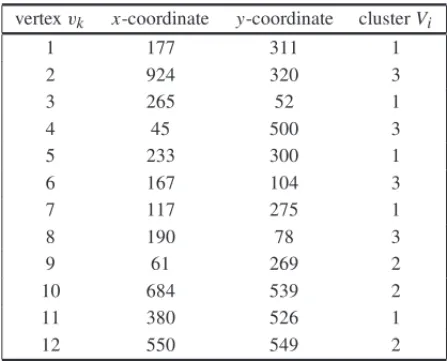
Table 1– Data for an example of the Algorithm 2.

vertexvk x-coordinate y-coordinate clusterVi

1 177 311 1

2 924 320 3

3 265 52 1

4 45 500 3

5 233 300 1

6 167 104 3

7 117 275 1

8 190 78 3

9 61 269 2

10 684 539 2

11 380 526 1

12 550 549 2

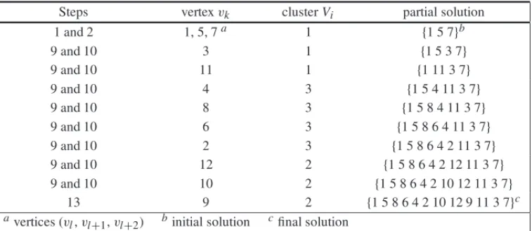
Table 1 presents the data of a small size instance containing 12 vertices and 3 clusters. In the first column shows o vertex vk, in the second the x-coordinate of vertex vk, in the third y -coordinate of vertexvk, and in the last column the clusterVi of vertexvk. This instance is con-sidered to illustrate how Algorithm 2 works, as shown in Table 2. It shows the some steps of the Algorithm 2 with data of Table 1. In the first column shows the steps, in the second the inserting the initial vertices (vl,vl+1,vl+2) or vertexvk, in the third the clusterVi of initial vertices or of vertexvk, and the last column the initial, partial or final solution. In this case, the initial partial tour is composed of vertices 1, 5 and 7, all belonging to cluster 1. Next, vertex 3 is inserted be-tween vertices 5 and 7. The procedure is repeated until vertex 9 is inserted and afeasible initial solutionis built.

Table 2– Steps of the Algorithm 2 with data of Table 1.

Steps vertexvk clusterVi partial solution

1 and 2 1, 5, 7a 1 {1 5 7}b

9 and 10 3 1 {1 5 3 7}

9 and 10 11 1 {1 11 3 7}

9 and 10 4 3 {1 5 4 11 3 7}

9 and 10 8 3 {1 5 8 4 11 3 7}

9 and 10 6 3 {1 5 8 6 4 11 3 7}

9 and 10 2 3 {1 5 8 6 4 2 11 3 7}

9 and 10 12 2 {1 5 8 6 4 2 12 11 3 7}

9 and 10 10 2 {1 5 8 6 4 2 10 12 11 3 7}

13 9 2 {1 5 8 6 4 2 10 12 9 11 3 7}c

a_{vertices (v}

l,vl+1,vl+2) binitial solution cfinal solution

procedureCheapinserts a vertexvk between two adjacent vertices (vi,vi+1) using the

cheap-est insertion criterion. N2thus consists in applying theDropprocedure followed by theCheap

procedure. The moves ofN2are applied until no further improvement of the procedures (Drop and Cheap) is found. The third neighborhood structure,N3, is based on vertex-exchange

move-ments in the same cluster (2-Swap). The fourth neighborhood structure,N4, uses the well-known

2-opt procedure both inside and between the clusters. In this work, we apply thefirst improve-mentstrategy forN1andN3, with a view of reducing the computational time, and the thebest improvementstrategy forN2andN4.

The double-bridge Martin, Otto & Felten [31] was adopted as one of theperturbation mecha-nisms. It consists of deleting four arcs and inserting another four in such a way that a new feasible solution is built. This perturbation, calledPert, is only applied inside a cluster, with more than eight vertices, which is selected at random. For the remaining cases, i.e, when the clusters have less or equal than eight vertices, we introduce another perturbation mechanism, calledPerttc, which randomly choosestwo clustersand modify their visiting order. In this case, the proce-dure does modify the visiting order of vertices inside the clusters. Such perturbations are called individually at a time, that is, they are never combined.

5 COMPUTATIONAL RESULTS

The set of instances used in Mestria, Ochi & Martins [33] were used to evaluate the performance of the proposed hybrid heuristic. These instances are available on-line athttp://labic.ic. uff.br/Instance/index.php. Six different classes of instances were considered.

Class 2: instances adapted from those found in Johnson & McGeoch [22] where the clusters were created by grouping the vertices in geometric centers.

Class 3: instances generated using the Concorde interface available in Applegate, Bixby, Chv´atal & Cook [2].

Class 4: instances generated using the layout proposed in Laporte, Potvin & Quilleret [25].

Class 5: instances similar toClass 2, but generated with different parameters.

Class 6: instances adapted from the TSPLIB Reinelt [38], where the rectangular floor plan is divided into several quadrilaterals and each quadrilateral corresponds to a cluster.

We chose a set of small, medium and large size instances. The set of small instances is composed of 27 test-problems from Class 1. The set of medium instances is composed of 3 instances from each of the six classes, which leads to a total of 18 instances. Finally, the last set is composed of 15 instances, more specifically, 5 from classes 4, 5 and 6, respectively. In this way, we have a variety of different classes of instances with varying sizes. Each class has one different granularity (the vertices are positioned and dispersed in various ways).

The empirical performance of HHGILS was compared with the optimal solution or the lower bound obtained by a Mixed Integer Programming (MIP) formulation proposed in Chisman [6]. The Parallel ILOG CPLEX was used a MIP solver, with four threads. The classes of cuts used in the CPLEX were clique cuts, cover cuts, implied bound cuts, flow cuts, mixed integer rounding cuts, and Gomory fractional cuts. The tests were executed in a 2.83 GHz Intel Core 2 Quad with 4 cores and 8 GB of RAM running Ubuntu Linux (kernel version 4.3.2-1). The HHGILS algorithm was coded inCprogramming language and it was executed in the same environment mentioned above, but in this case only a single thread was used.

The main parameters used in our testing are described as follows. Eleven values were used for αk and they were initially chosen with uniform probability from the interval {0.0,0.1,0.2, . . . ,1.0}. The parameter maxint was set to 35, maxext (maximum number of external itera-tions) set to 40, andmaxprobwas set to 10. HHGILS was executed ten times for each instance. These parameters were calibrated after preliminary experiments.

5.1 Comparison with CPLEX

Table 3 shows the results found in the set of instances of Class 1, where the first column contains the instances. The instances XX-name_{YYYis composed ofXXclusters, one name}name_{, and} YYYvertices, for example, (a) the instance 5-eil51 is composed of five clusters and 51 vertices (first row of Table 3 with the results), (b) the instance 10-eil51 is composed of ten clusters and 51 vertices (second row), (c) the instance 75-lin105 is composed 75 clusters and 105 vertices (last row), and so on. The second column contains the optimal values obtained by CPLEX and the third column the time (in seconds) required by CPLEX to find the optimal solution, i.e., the CPLEX was carry out until to find the optimal solution withgap equal a 0 (zero). The gap

Table 3– Comparison between HHGILS and CPLEX for the small size instances of Class 1.

CPLEX HHGILS

Instances

Opt Time (s) Gap(%) Time (s)

5-eil51 437 12.31 0.00 3.80

10-eil51 440 74.38 0.00 5.50

15-eil51 437 2.04 0.00 5.00

5-berlin52 7991 201.80 0.11 4.50

10-berlin52 7896 89.17 0.52 5.10

15-berlin52 8049 75.93 0.00 4.00

5-st70 695 13790.11 0.00 6.90

10-st70 691 4581.00 0.43 3.70

15-st70 692 883.50 0.87 6.40

5-eil76 559 83.70 0.00 5.10

10-eil76 561 254.30 1.07 8.60

15-eil76 565 49.66 0.88 6.80

5-pr76 108590 99.29 0.00 6.30

10-pr76 109538 238.13 0.00 8.30

15-pr76 110678 261.94 0.00 9.70

10-rat99 1238 650.67 0.00 12.60

25-rat99 1269 351.15 0.00 21.40

50-rat99 1249 2797.58 0.00 18.60

25-kroA100 21917 3513.57 0.00 21.70

50-kroA100 21453 947.55 0.00 21.70

10-kroB100 22440 4991.44 0.91 12.40

50-kroB100 22355 2579.22 0.00 22.40

25-eil101 663 709.45 1.06 21.10

50-eil101 644 275.33 0.16 20.80

25-lin105 14438 6224.55 1.38 16.70

50-lin105 14379 1577.21 0.00 22.60

75-lin105 14521 15886.77 0.00 23.70

Average values 2266.73 0.27 12.05

HHGILS and the optimal solution. The last column shows the average computing time (in sec-onds) of HHGILS. The stopping criterion of HHGILS in this case was the number of iterations. The boldface values indicate that the hybrid heuristic found the optimal solution. From Table 3, it can be seen that HHGILS found 17 optimal solutions out of 27 instances. The average gap between the solutions obtained by HHGILS and the optimal ones was 0.27%, whereas the aver-age computing time was 12.05 seconds. In this case, the perturbationPerttcwas used in 11 of the 27 instances.

gap=100∗

_{best −lb}

best+ǫ

, (10)

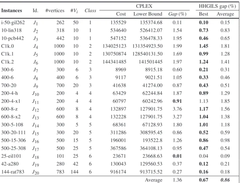
In Table 4, we present the computational results obtained by CPLEX and HHGILS for medium size instances. The first column contains the names of the instances and in the second their identifiers, followed by the number of vertices, number of clusters and the Class of the instances. The next three columns show the upper bound, the lower bound and the gap found by CPLEX. The last two columns show the best and average gaps found by HHGILS with respect to the lower bound obtained by CPLEX. We set a time limit of 7200 seconds for all CPLEX executions. The stopping criterion for HHGILS was set to 720 seconds. As already mentioned, the hybrid heuristic was executed ten times for each instance, leading to a total time of 7200 seconds.

On average, the best and average solutions found by HHGILS are less than 1% away from the lower bounds obtained by CPLEX, which suggests that the proposed hybrid heuristic had a robust performance, in terms of solution quality, on this set of instances.

It should be noticed that, for the set of small instances, the worst average gap found by HHGILS, with respect to the optimal solutions, was 1.38%, whereas the worst average gap for the medium instances, with respect to the lower bound, was 1.45%. To our knowledge, the best CTSP α-approximation algorithm proposed in the literature is the one presented in Bao & Liu [4], with an approximation factor of 13/6 (≈2.17). Therefore, it is possible to observe that the largest gaps found by HHGILS are much smaller than the approximation factor obtained in Bao & Liu [4].

Table 4– Comparison between HHGILS and CPLEX for medium size instances.

CPLEX HHGILS gap (%)

Instances Id. #vertices #Vi Class _{Cost Lower Bound Gap(%) Best Average}

i-50-gil262 J1 262 50 1 135529 135374.68 0.11 0.10 0.15

10-lin318 J2 318 10 1 534640 526412.07 1.54 0.73 0.83

10-pcb442 J3 442 10 1 547152 536478.33 1.95 0.46 0.65

C1k.0 J4 1000 10 2 134025123 131354923.50 1.99 1.45 1.81

C1k.1 J5 1000 10 2 130750874 128540131.50 1.69 0.99 1.28

C1k.2 J6 1000 10 2 144341485 141501445 1.97 1.24 1.41

300-6 J7 300 6 3 8969 8915.18 0.60 0.21 0.31

400-6 J8 400 6 3 9117 9021.51 1.05 0.33 0.46

700-20 J9 700 20 3 41638 41274.00 0.87 0.43 0.51

200-4-h J10 200 4 4 63429 62244.84 1.87 0.89 1.29

200-4-x1 J11 200 4 4 60797 60242.96 0.91 1.13 1.85

600-8-z J12 600 8 4 132897 127901.75 3.76 1.17 1.56

600-8-x2 J13 600 8 4 132228 127901.75 3.27 1.04 1.38

300-5-108 J14 300 5 5 68361 67128.93 1.80 1.01 1.18

300-20-111 J15 300 20 5 311286 308595.45 0.86 0.52 0.59

500-15-306 J16 500 15 5 196001 193522.8 1.26 0.86 0.98

500-25-308 J17 500 25 5 367586 364108.13 0.95 0.47 0.54

25-eil101 J18 101 25 6 23671 23668.63 0.01 0.04 0.09

42-a280 J19 280 42 6 130043 129560.53 0.37 0.12 0.21

144-rat783 J20 783 144 6 916174 913715.52 0.27 0.16 0.18

5.2 Results obtained by the hybrid heuristic HHGILS for large size instances

Table 5 illustrates the best and average results obtained by HHGILS for large size instances using a stopping criterion of 1080 seconds for each run. The first column contains the names of the instances and the second column their identifiers, followed by the number of vertices, number of clusters and the Class of the instances. The sixth and seventh columns show the values obtained by HHGILS. These results appear to be quite competitive when compared to other approaches from the literature as shown later in Table 8.

Table 5– The best and average results obtained by HHGILS for large size instances.

Instances Id. #vertices #Vi Class Best Average

49-pcb1173 J21 1173 49 6 67043 68260.70

100-pcb1173 J22 1173 100 6 68786 70640.83

144-pcb1173 J23 1173 144 6 66830 69084.25

10-nrw1379 J24 1379 10 6 63620 64643.88

12-nrw1379 J₂₅ 1379 12 6 63558 64741.57

1500-10-503 J26 1500 10 5 11986 12109.45

1500-20-504 J27 1500 20 5 17107 17315.72

1500-50-505 J28 1500 50 5 25264 25558.90

1500-100-506 J29 1500 100 5 32260 33760.64

1500-150-507 J30 1500 150 5 37658 38433.09

2000-10-a J31 2000 10 4 116254 116881.38

2000-10-h J32 2000 10 4 36447 37305.14

2000-10-z J33 2000 10 4 37059 37443.69

2000-10-x1 J34 2000 10 4 36752 37704.03

2000-10-x2 J₃₅ 2000 10 4 36660 37117.11

5.3 Comparison with other heuristic algorithms and an exact method

We now compare our results with those reported in Mestria, Ochi & Martins [33]. More pre-cisely, we compare HHGILS with the following methods: GPR1R2, GPR4 and G. The first two consist of a combination between GRASP and Path Relinking while the third one is the traditional GRASP. According to the experiments performed in Mestria, Ochi & Martins [33], GPR1R2 outperforms all other methods proposed in that paper. The other two methods also ob-tained satisfactory results but only in a particular class of instances. Therefore, GPR1R2 will be considered in all comparisons, while GPR4 and G will only be considered in some partic-ular cases. It is important to mention that GPR1R2, GPR4 and G were executed in the same computational environment of HHGILS.

Table 6 – Comparison between HHGILS and GPR1R2 Mestria, Ochi & Martins [33] for the small instances of Class 1.

HHGILS GPR1R2

Instances

Gap(%) Time (s) Gap(%) Time (s)

5-eil51 0.00 3.80 0.00 1.00

10-eil51 0.00 5.50 0.00 1.00

15-eil51 0.00 5.00 0.00 1.00

5-berlin52 0.11 4.50 0.00 1.20

10-berlin52 0.52 5.10 0.00 1.10

15-berlin52 0.00 4.00 0.00 1.10

5-st70 0.00 6.90 0.00 2.30

10-st70 0.43 3.70 0.00 2.00

15-st70 0.87 6.40 0.00 2.00

5-eil76 0.00 5.10 0.36 2.70

10-eil76 1.07 8.60 0.53 2.40

15-eil76 0.88 6.80 0.35 2.50

5-pr76 0.00 6.30 0.00 2.70

10-pr76 0.00 8.30 0.00 2.20

15-pr76 0.00 9.70 0.15 2.30

10-rat99 0.00 12.60 0.00 4.90

25-rat99 0.00 21.40 0.63 4.70

50-rat99 0.00 18.60 0.72 4.90

25-kroA100 0.00 21.70 0.00 4.70

50-kroA100 0.00 21.70 0.00 5.20

10-kroB100 0.91 12.40 0.16 4.80

50-kroB100 0.00 22.40 1.33 5.20

25-eil101 1.06 21.10 1.36 4.60

50-eil101 0.16 20.80 1.09 5.40

25-lin105 1.38 16.70 0.00 5.10

50-lin105 0.00 22.60 1.08 5.70

75-lin105 0.00 23.70 0.59 6.40

Average values 0.27 12.05 0.25 3.30

In Table 7 we compare the gaps between the best solutions obtained by HHGILS, GPR1R2 and GPR4 and the lower bounds found by CPLEX on instances of Mestria, Ochi & Martins [33]. The stopping criterion for all methods is 720 seconds for each of the 10 executions.

Table 7– Comparison between HHGILS, GPR1R2 Mestria, Ochi & Martins [33] and GPR4 Mestria, Ochi & Martins [33] for medium size instances.

Best gap (%) Average gap (%)

Instances

HHGILS GPR1R2 GPR4 HHGILS GPR1R2 GPR4

10-lin318 0.73 0.76 0.84 0.83 1.18 1.65

10-pcb442 0.46 0.66 0.66 0.65 1.22 1.52

C1k.0 1.45 1.60 1.68 1.81 1.76 1.81

C1k.1 0.99 1.27 1.27 1.28 1.42 1.46

300-6 0.21 0.49 0.50 0.31 0.78 1.04

700-20 0.43 0.64 0.61 0.51 0.72 0.72

200-4-h 0.89 1.19 1.24 1.29 2.30 3.31

600-8-z 1.17 1.96 1.95 1.56 2.54 2.63

300-20-111 0.52 0.43 0.44 0.59 0.63 0.78

500-25-308 0.47 0.58 0.61 0.54 0.73 0.76

25-eil101 0.04 0.03 0.03 0.09 0.18 0.33

144-rat783 0.16 0.20 0.19 0.18 0.24 0.24

Average values 0.67 0.82 0.83 0.80 1.14 1.35

Finally, Table 8 presents a comparison between the best and average results found by HHGILS, G, and GPR1R2 on large size instances. In this case we report the gaps between the solution found by the respective method and the best solution values found by GPR1R2.

The stopping criterion for the hybrid heuristics was set to 1080 seconds for each run. The first column contains the identifiers of the instances, the second and third columns the results obtained by the GPR1R2 heuristic, followed by the gaps of the best solution and the average solution of the methods.

From Table 8, we can observe that HHGILS found better solutions when compared to G and GPR1R2, except for the instanceJ28. With respect to the best solution values, HHGILS obtained

an average gap of−2.93%, whereas G obtained 0.35%. As for the average solutions, HHGILS obtained an average gap of−3.83%, while G obtained 1.57%.

We also compare our results with an exact method by the Concorde solver, reported in Applegate, Bixby, Chv´atal & Cook [2] through of instances of Class 3 (instances generated using its own user interface). Table 9 shows the results found in the set of instances of Class 3, where the first column contains the instances. The instancesXXXX-YYis composed ofXXXXvertices andYYY

Table 8– Comparison between HHGILS, G Mestria, Ochi & Martins [33] and GPR1R2 Mestria, Ochi & Martins [33] for large size instances.

GPR1R2 Results Best gap (%) Average gap (%) Id.

Best Average HHGILS G HHGILS G

J21 70651 73311.92 -5.11 0.40 -6.89 2.94

J22 72512 74871.65 -5.14 0.54 -5.65 2.87

J₂₃ 72889 74621.57 -8.31 0.08 -7.42 2.68

J24 66747 68955.78 -4.68 0.66 -6.25 2.33

J25 66444 69141.16 -4.34 0.26 -6.36 2.96

J₂₆ 12278 12531.44 -2.38 0.32 -3.37 1.03

J27 17252 17589.12 -0.84 0.06 -1.55 1.36

J28 25124 25761.53 0.56 0.03 -0.79 0.65

J29 33110 33692.73 -2.57 0.52 0.20 1.19

J30 38767 39478.00 -2.86 0.01 -2.65 0.43

J31 116473 118297.46 -0.19 0.86 -1.20 0.53

J32 37529 38861.78 -2.88 0.25 -4.01 1.11

J33 37440 38765.91 -1.02 0.17 -3.41 1.29

J34 37262 39253.08 -1.37 0.91 -3.95 0.49

J35 37704 38699.53 -2.77 0.19 -4.09 1.64

Average values – – -2.93 0.35 -3.83 1.57

the computing time (in seconds) of HHGILS. For the specific case, we set a time limit for all HHGILS executions, as the stopping criterion.

From Table 9, it can be seen that HHGILS found good solutions. The boldface values indicate that the algorithms carry out in less time. Table 9 shows strong robustness of our hybrid heuristic. The average gap between the solutions obtained by HHGILS and the best ones was 6.46%, whereas the average computing time was 43.33seconds. The results from Table 9 show that HHGILS reached good results in a short period of time. Thus, the HHGILS allows for greater freedom of decision-making in operational planning in automated warehouse routing, emergency vehicle dispatching, production planning, vehicle routing, among others.

6 CONCLUSIONS

Table 9– Comparison between HHGILS and Concorde Applegate, Bixby, Chv´atal & Cook [2] for the instances of Class 3.

Concorde HHGILS

Instances

Best Time (s) Gap(%) Time (s)

300-6 774 21.00 1.94 15.00

350-6 894 27.79 5.59 15.00

400-6 885 58.88 4.52 15.00

450-6 945 34.77 6.46 15.00

500-6 1063 41.08 6.49 15.00

550-20 1419 51.55 4.09 45.00

600-20 1475 50.02 6.10 45.00

650-20 1545 71.03 5.57 45.00

700-20 1625 69.47 6.77 45.00

750-25 1694 23.89 7.50 45.00

800-25 1784 30.61 6.39 70.00

850-25 1882 114.19 6.59 70.00

900-25 1949 38.50 9.08 70.00

950-30 2072 121.58 9.89 70.00

1000-30 2144 61.99 9.93 70.00

Average values 54.42 6.46 43.33

The CTSP has many applications in real life, for example, automated warehouse routing, emer-gency vehicle dispatching, production planning, vehicle routing, commercial transactions with supermarkets and shops and grocery suppliers and so on. This applications, set of small size in-stances, need to be solved by heuristic algorithm for rapid response to the operational planning process. In this paper we proposed the hybrid heuristic algorithm (HHGILS) for this applications with the best performance and high-quality solutions in a reasonable computational time.

We compare the results found by HHGILS with other GRASP based methods from the literature for small, medium and large size instances. It was observed that the method which combines GRASP with Path Relinking (GPR1R2) Mestria, Ochi & Martins [33] found, on average, better solutions for small size instances, but HHGILS outperformed such method when considering medium and large size instances. Our hybrid heuristic also was compared with an exact method and it presented robustness.

We observe that the largest gap (0.0376) found by HHGILS was much smaller than the approxi-mation factor obtained in Bao & Liu [4], a new approxiapproxi-mation algorithm with a factor of 13/6.

ACKNOWLEDGEMENTS.

This paper has been partially supported by the Instituto Federal de Educac¸˜ao, Ciˆencia e Tecnolo-gia do Esp´ırito Santo (IFES). This acknowledgment extends to Prof. Anand Subramanian for your comments.

References

[1] ANILYS, BRAMELJ & HERTZA. 1999. A 5/3-approximation Algorithm for the Clustered Traveling Salesman Tour and Path Problems.Operations Research Letters,24(1-2): 29–35.

[2] APPLEGATED, BIXBYR, CHVATAL´ V & COOKW. 2007. Concorde TSP Solver. William Cook, School of Industrial and Systems Engineering, Georgia Tech.http://www.tsp.gatech.edu/ concorde/index.html. Accessed 22 December 2007.

[3] ARKINEM, HASSINR & KLEINL. 1997. Restricted Delivery Problems on a Network.Networks, 29(4): 205–216.

[4] BAOX & LIUZ. 2012. An improved approximation algorithm for the clustered traveling salesman problem.Information Processing Letters,112(23): 908–910.

[5] CASERTAM & VOSSS. 2010. Matheuristics: Hybridizing Metaheuristics and Mathematical Pro-gramming, Springer US, Boston, MA, chap Metaheuristics: Intelligent Problem Solving, pp. 1–38.

[6] CHISMANJA. 1975. The clustered traveling salesman problem.Computers & Operations Research, 2(2): 115–119.

[7] CHRISTOFIDESN. 1976. Worst-case Analysis of a new Heuristic for the Travelling Salesman Prob-lem. Technical Report 388, Graduate School of Industrial Administration, Carnegie-Mellon Univer-sity.

[8] DINGC, CHENGY & HEM. 2007. Two-Level Genetic Algorithm for Clustered Traveling Salesman Problem with Application in Large-Scale TSPs.Tsinghua Science & Technology,12(4): 459–465.

[9] DONGG, GUOWW & TICKLEK. 2012. Solving the traveling salesman problem using cooperative genetic ant systems.Expert Systems with Applications,39(5): 5006–5011.

[10] ESCARIOJB, JIMENEZJF & GIRON-SIERRAJM. 2015. Ant colony extended: Experiments on the travelling salesman problem.Expert Systems with Applications,42(1): 390–410.

[11] FEOT & RESENDEM. 1995. Greedy Randomized Adaptive Search Procedures.Journal of Global

Optimization,6(2): 109–133.

[12] FESTAP & RESENDEM. 2011. GRASP: basic components and enhancements.Telecommunication

Systems,46(3): 253–271.

[14] GENDREAUM, LAPORTEG & POTVINJY. 1994. Heuristics for the Clustered Traveling Salesman Problem. Technical Report CRT-94-54, Centre de recherche sur les transports, Universit´e de Montr´eal, Montr´eal, Canada.

[15] GENDREAUM, LAPORTEG & HERTZ A. 1997. An Approximation Algorithm for the Traveling Salesman Problem with Backhauls.Operations Research,45(4): 639–641.

[16] GHAZIRIH & OSMANIH. 2003. A Neural Network for the Traveling Salesman Problem with Back-hauls.Computers & Industrial Engineering,44(2): 267–281.

[17] GLOVERF, LAGUNAM & MART´IR. 2004. Scatter Search and Path Relinking: Foundations and Advanced Designs. In: ONWUBOLUGC & BABUBV (eds.) New Optimization Techniques in Engi-neering, Springer-Verlag, Heidelberg, pp. 87–100.

[18] GUTTMANN-BECKN, HASSINR, KHULLERS & RAGHAVACHARIB. 2000. Approximation Algo-rithms with Bounded Performance Guarantees for the Clustered Traveling Salesman Problem.

Algo-rithmica,28(4): 422–437.

[19] HANSENP & MLADENOVIC´ N. 2001. Variable neighborhood search: Principles and applications.

European Journal of Operational Research,130(3): 449–467.

[20] HANSEN P & MLADENOVIC´ N. 2003. Variable Neighborhood Search. In: GLOVER FW & KOCHENBERGERGA (eds.) Handbook of Metaheuristics, London: Kluwer Academic Publisher, Boston, Dordrecht, pp. 145–184.

[21] HOOGEVEENJA. 1991. Analysis of Christofides’ Heuristic: Some Paths are more Difficult than Cycles.Operations Research Letters,10(5): 291–295.

[22] JOHNSONDS & MCGEOCHLA. 2002. Experimental Analysis of Heuristics for the STSP. In: GUTING & PUNNENA (eds.) The Traveling Salesman Problem and its Variations, Kluwer Aca-demic Publishers, Dordrecht, Holanda, pp. 369–443.

[23] JONGENSK & VOLGENANT T. 1985. The Symmetric Clustered Traveling Salesman Problem.

European Journal of Operational Research,19(1): 68–75.

[24] LAPORTEG & PALEKARU. 2002. Some Applications of the Clustered Travelling Salesman

Prob-lem.Journal of the Operational Research Society,53(9): 972–976.

[25] LAPORTEG, POTVINJY & QUILLERETF. 1996. A Tabu Search Heuristic using Genetic Diversifi-cation for the Clustered Traveling Salesman Problem.Journal of Heuristics,2(3): 187–200.

[26] L ´ETOCART L, PLATEAUMC & PLATEAUG. 2014. An efficient hybrid heuristic method for the 0-1 exact k-item quadratic knapsack problem.Pesquisa Operacional,34: 49–72.

[27] LOKINFCJ. 1979. Procedures for Travelling Salesman Problems with Additional Constraints.

Euro-pean Journal of Operational Research,3(2): 135–141.

[29] LOURENC¸OHR, MARTINOC & STUTZLE¨ T. 2002. Iterated Local Search. In: Glover F & Kochen-berger G (eds.) Handbook of Metaheuristics, Kluwer Academic Publishers, Boston, pp. 321–353.

[30] LOURENC¸O HR, MARTIN OC & STUTZLE¨ T. 2010. Handbook of Metaheuristics, Springer US, Boston, MA, chap Iterated Local Search: Framework and Applications, pp. 363–397.

[31] MARTINO, OTTOSW & FELTENEW. 1991. Large-Step Markov Chains for the Traveling Salesman Problem.Complex Systems,5: 299–326.

[32] MART´INEZDA, ALVAREZ-VALDESR & PARRENO˜ F. 2015. A grasp algorithm for the container loading problem with multi-drop constraints.Pesquisa Operacional,35(1): 1–24.

[33] MESTRIAM, OCHILS & MARTINSSL. 2013. Grasp with path relinking for the symmetric eu-clidean clustered traveling salesman problem.Computers & Operations Research,40(12): 3218– 3229.

[34] MILLER CE, TUCKERAW & ZEMLIN RA. 1960. Integer Programming Formulation of Travel-ing Salesman Problems.Journal of the ACM,7(4): 326–329. DOI:http://doi.acm.org/10. 1145/321043.321046.

[35] NAGATA Y & SOLER D. 2012. A new genetic algorithm for the asymmetric traveling salesman problem.Expert Systems with Applications,39(10): 8947–8953.

[36] POTVINJY & GUERTINF. 1995. A Genetic Algorithm for the Clustered Traveling Salesman Prob-lem with an A Priori Order on the Clusters. Technical Report CRT-95-06, Centre de recherche sur les transports, Universit´e de Montr´eal, Canada.

[37] POTVINJY & GUERTINF. 1996. The clustered traveling salesman problem: A genetic approach. In: OSMANIH & KELLYJ (eds). Meta-heuristics: Theory & Applications, Kluwer Academic Pub-lishers, Norwell, MA, USA, chap 37, pp. 619–631.

[38] REINELTG. 2007. TSPLIB. Universit¨at Heidelberg, Institut f¨ur Informatik, Heidelberg, Germany http://www.iwr.uni-heidelberg.de/groups/comopt/software/TSPLIB95/

index.html. Accessed 17 September 2007.

[39] STUTZLE¨ T. 2006. Iterated local search for the quadratic assignment problem.European Journal of

Operational Research,174(3): 1519–1539.

[40] SUBRAMANIANA & BATTARRAM. 2013. An Iterated Local Search algorithm for the Travelling Salesman Problem with Pickups and Deliveries.Journal of the Operational Research Society, 64: 402–409.

[41] VIDALT, BATTARRAM, SUBRAMANIANA & ERDOGANG. 2015. Hybrid Metaheuristics for the Clustered Vehicle Routing Problem.Computers & Operations Research,58(C): 87–99.

[42] WEINTRAUB A, ABOUDJ, FERNANDEZC, LAPORTEG & RAMIREZE. 1999. An Emergency

Vehicle Dispatching System for an Electric Utility in Chile.Journal of the Operational Research