STOCHASTIC BENDERS DECOMPOSITION FOR THE SUPPLY CHAIN INVESTMENT PLANNING PROBLEM UNDER DEMAND UNCERTAINTY
Fabricio Oliveira and Silvio Hamacher
∗Received March 6, 2012 / Accepted September 7, 2012
ABSTRACT.This paper presents the application of a stochastic Benders decomposition algorithm for the problem of supply chain investment planning under uncertainty applied to the petroleum byproducts supply chain. The uncertainty considered is related with the unknown demand levels for oil products. For this purpose, a model was developed based on two-stage stochastic programming. It is proposed two different solution methodologies, one based on the classical cutting plane approach presented by Van Slyke & Wets (1969), and other, based on a multi cut extension of it, firstly introduced by Birge & Louveaux (1988). The methods were evaluated on a real sized case study. Preliminary numerical results obtained from computational experiments are encouraging.
Keywords: supply chain investment planning, stochastic optimization, stochastic Benders decomposition.
1 INTRODUCTION
Oil companies are global multinational organizations whose decisions involve a large number of factors related to the supply of raw materials, their processing and distribution. For compa-nies with strongly diversified sources of petroleum supply, a long cast of products, and multiple markets, the advance planning of all activities along the supply chain is vital. Such planning includes the definition of production levels of oil (from oil fields) and of petroleum byproducts (from oil refineries), as well as the distribution among these refineries and to the final consumers of oil products. Major oil companies are characterized by integrated and verticalized activi-ties, and the activities of refining and distributing oil products are characterized by low profit margins. Therefore, techniques for decision-making optimization are frequently used in the con-text of the oil supply chain.
The use of optimization techniques for supply chain design and planning has already been observed in the literature since the 1970’s, especially the in seminal works of Geoffrion &
*Corresponding author
Graves (1974). Vidal & Goetschalckx (1997) and Beamon (1998) present an extensive litera-ture review on supply chain models. Although the research literalitera-ture on the strategic modeling of supply chains is quite rich, few studies have included uncertainty mitigation in addition to other decisions of financial scope, such as commercialization income, market considerations and investment planning. According to Sahinidis (2004), the incorporation of uncertainty into plan-ning models using stochastic optimization remains a challenge due to the large computational requirements involved.
For nearly 50 years, companies in the oil and chemical industries have led the development and use of mixed integer linear programming to support decision making at all levels of planning. An overriding feature in the oil industry is its wide range of uncertainties, typically related to the unpredictable levels of demand for refined products, fluctuations in prices in domestic and international markets and inaccuracies in the forecasted production of oil and gas. For this reason, many works have used techniques based on mathematical programming to support decision-making under uncertainty (Escuderoet al., 1999; Dempsteret al., 2000; Al-Othmanet al., 2008; Khoret al., 2008).
Due to the great level of uncertainties taken into consideration, and the fact that the aforemen-tioned problem is modeled as a mixed-integer linear program, it might become computationally infeasible to deal with a great number of scenarios by solving deterministic equivalents of the stochastic problems. Therefore, a decomposition approach might turn out to be a valid alternative as solution methodology.
The first approaches using decomposition schemes for stochastic programs were presented by Van Slyke & Wets (1969), a framework based on Benders decomposition (Benders, 1962) applied to two-stage stochastic problems, which became known as the L-Shaped method. Birge & Louveaux (1988) report an extension of the method presented by Van Slyke & Wets (1969), exploiting the structure of two-stage stochastic problems to place several cuts at once at each major iteration.
Cutting-plane schemes has been successfully used in solving large-scale problems since the pioneering paper of Geoffrion & Graves (1974),e.g., the uncapacitated network design problem with undirected arcs (Magnantiet al., 1986, Costaet al., 2012), the stochastic transportation-location problems (Franca, 1982), the locomotive and car assignment problem (Cordeauet al., 2000; Cordeau et al., 2001), the non-convex water resource management problem (Caiet al., 2001), hub location problem (Miranda Junioret al., 2011), to name a few.
The paper is organized as follows: Section 2 describes the proposed mathematical model; Sec-tion 3 presents the tradiSec-tional primal decomposiSec-tion framework, while SecSec-tion 4 presents the multi cut framework; computational results are shown in Section 5; Section 6 draws some conclusion.
2 PROBLEM STATEMENT
The problem approached in this paper can be defined as the strategic planning of petroleum products distribution, where one seeks to select investments to be made in logistics infrastruc-ture, taking into consideration decisions regarding the distribution of flows, inventory policies, and the level of the external commercialization. Such decisions arise in the context of strategic and tactical planning faced by petroleum products distribution companies operating over large geographical regions. We consider this problem as an integrated distribution network design and binary capacity expansion problem under a multi-product and multi-period setting.
Petroleum products from refineries are stored in tanks to be directed to distribution bases. These bases serve as negotiation points with distributors and are considered as aggregation points of demand for such products. They also might serve as an intermediate point for other bases further away from the refineries. The bases are capable of storing product when necessary, given that the problem is considered under a multi-period operation. The storage and throughput capacities of the bases are limited. However, they can be improved through an expansion project. The same idea holds for arcs, which can also be expanded in the same fashion. In addition to that, we also consider the possibility of building new arcs and bases. The tanks of these bases are constantly being loaded and unloaded. This process is known as the tank rotation and is subject to the physical limitations that are inherent in the hardware associated with the tanks of the distribution base. The rotating capacity refers to the number of times a tank can be filled and emptied over a certain period of time.
For modeling the uncertainty we propose a two-stage mixed-integer linear stochastic program-ming model. The uncertainty is represented through the consideration of discrete scenarios. These scenarios are defined by means of sampling from a continuous distribution of the demand levels for a given product at a certain base. Further details regarding the scenario generation process can be found in Oliveira & Hamacher (2012).
The first-stage decisions are the selection of the expansion projects for tanks and arcs, as well as their timing. These decisions are represented by binary variables. Typically, these investments are highly capital intensive and are built-to-order due to their technical complexity and particular specifications. For this reason, we assume that the same investment can only be implemented once along the time horizon. Also, we assume that investment decisions are available for use at the beginning of the selected time period.
The objective function consists of investments costs of tanks and arcs expansion projects and the expected costs related to freight, inventory, and emergency floating tank acquisition. The purpose of the model is to plan the transportation and inventory decisions that will cope with the projected (although uncertain) growth of product demands, together with the possible investments that should be implemented and when, minimizing both investment and expected logistics costs.
3 MATHEMATICAL MODEL
The notation to be used for the presentation of the mathematical model is given below. For the sake of notational compactness, the domains of summations will be omitted, except when the summation is evaluated only on a subset of the natural domain. When there is no mention of this fact, its domain should be considered as the original set to which the index refers. In addition to that, we use bold caption to represent decision variable vectors.
Indexes
i,j,l∈N – Locations
p∈P – Products
t ∈T – Time periods
ξ ∈ – Uncertainty realizations
Sets
B ⊆N – Subsets of distribution bases
N – Locations
P – Products
S⊆N – Subset of suppliers
T – Time periods
– Uncertainty possible realizations
Parameters
A0i j – Current arc capacity
Ai j – Additional arc capacity
Ci jt – Transportation cost
Dtj p(ξ ) – Demand
Hj p – Inventory cost
Kj p – Maximum number of tank rotations
M0j p – Current inventory capacity
Mj p – Additional inventory capacity
Stj p – Shortfall cost
Wtj p – Inventory investment cost
Yi jt – Arc investment cost
Variables
xi j pt (ξ ) – Product flow
vtj p(ξ ) – Inventory level
utj p(ξ ) – Unmet demand
yi jt – Arc investment decision
wtj p – Location investment decision
The mathematical model for the optimization of aforementioned problem can be stated as follows:
min
w,y∈{0,1} X
j,p,t
Wtj pwtj p+X
i,j,t
Yi jt yi jt +Q(w,y) (1)
s.t. X
t
wtj p≤1, ∀ j,p (2)
X
t
yi jt ≤1, ∀i,j (3)
where the termQ(w,y)=E[Q(w,y, ξ )]represents the expectation evaluated over allξ ∈ possible realizations for the uncertain parameters of the second-stage problem, given an invest-ment decision(w,y). Constraints (2) and (3) define that each investment can happens only once along the time horizon considered.
The second-stage problem Q(w,y, ξ )can be stated as follows in Eqs. (4) to (9). The objective function (4) represents freight costs between the nodes, inventory costs, and the cost of shortfall. Equation (5) comprises the material balance in distribution bases. Constraint (6) limits the supply availability at sources. Constraint (7) defines the arc capacities and the possibility of its expansion through the investment decisions y. In a similar way, constraint (8) defines the storage capacities together with its expansion possibility. Constraint (9) sets the throughput limit for bases, defined by the product of the available storage capacity with the maximum number of tank rotations.
min x,u,v∈R+
X
i,j,p,t
Ci jt xi j pt (ξ )+X
j,p,t
Hj pvtj p(ξ )+
X
j,p,t
Stj putj p(ξ ) (4)
s.t. X
i
xi j pt (ξ )+vtj p−1(ξ )+utj p(ξ )
=X
l
xtjl p(ξ )+vt
−1
j p (ξ )+D t
X
j
xi j pt (ξ )≤Oi pt , ∀i ∈S,p,t (6)
X
p
xi j pt (ξ )≤A0i j+Ai j
X
t′≤t
yi jt′, ∀i,j,t (7)
vtj p(ξ )≤ M0j p+Mj p
X
t′≤t
wtj p′ , ∀ j∈B,p,t (8)
X
i
xi j pt (ξ )≤Kj p
M0j p+Mj p
X
t′≤t wtj p′
, ∀ j∈B,p,t (9)
4 STOCHASTIC BENDERS DECOMPOSITION
The model proposed in the previous section can be defined as an optimization model with bi-nary first-stage variables, continuous second-stage variables and discrete random parameters. Moreover, the model has relatively complete recourse (Birge & Louveaux, 1997) that is, for any feasible first stage solution, the second stage problem is feasible. Such characteristics allow us a decomposition framework based on Benders decomposition (Benders, 1962) applied to stochas-tic optimization.
We start by noting that the so-called master problem can be equivalently reformulated as follows:
min
w,y∈{0,1} X
j,p,t
Wtj pwtj p+X
i,j,t
Yi jt yi jt +M (10)
s.t. X
t
wtj p ≤1, ∀ j,p (11)
X
t
yi jt ≤1, ∀i,j (12)
M ≥Q(w,y) (13)
This formulation allows one to distinguish an important issue. Inequality (13) cannot be used computationally as a constraint, since it is not defined explicitly, but only implicitly, by a number of optimization problems. The main idea of the proposed decomposition method is to relax this constraint and replace it by a number of cuts, which may be gradually added following an iterative solving process. These cuts, defined as supporting hyperplanes of the second-stage objective function, might eventually provide a good estimation for the value of Q(w,y)in a finite number of iterations.
Initialization: DefineL BandU Bas lower and upper bounds. SetL B = −∞andU B = ∞. DefineBas the iteration counter and setB =0. Let(wˆ,yˆ)denote the incumbent solution.
Step 1: Solve themaster problemand let(wB,yB)andL Bbe its optimal solution and optimal objective value respectively.
Step 2: For each realizationξ ∈solve the slave problem (4)-(9) stated before fixing(wB,yB) and calculate the value forQˆ(wB,yB)given by equation (14),
ˆ
Q(wB,yB)=X ξ∈
P(ξ )Q(wB,yB, ξ ) (14)
where P(ξ )is the probability of realizationξ occurs. LetF(w,y)represent the first-stage cost function and:
G(wB,yB)=F(wB,yB)+ ˆQ(wB,yB) (15)
IfG(wB,yB) < U B then update U B = G(wB,yB)and the incumbent solution (wˆ,ˆy) = (wB,yB).
Step 3: IfU B−L B≤ǫ, whereǫis a pre specified tolerance, then return the incumbent solution (wˆ,yˆ)andU Bas the objective function value. Otherwise, proceed toStep 4.
Step 4: Letα,β,γ,δ, andςbe the dual variables associated with constraints (5) to (9) respec-tively. Generate the cut (16):
M ≥X
i,j,t
ai jt
X
t′≤t
yti j′
+ X
j,p,t
btj p
X
t′≤t wtj p′
+K (16)
where:
ai jt = X ξ∈
P(ξ )Ai jγi jt(ξ )
btj p = X ξ∈
P(ξ )Mj p
h
δtj p+Kj pςtj p(ξ )
i
K = X
ξ∈
P(ξ )
X
j,p,t
αtj p(ξ )Dtj p(ξ )+βtj p(ξ )Otj p
+δtj p(ξ )M0j p+Kj pM0j pςtj p(ξ )
+X
i,j,t
γi jt(ξ )A0i j
Add the cut to themaster problem. Update B=B+1 and go tostep 1.
5 MULTI CUT STOCHASTIC BENDERS DECOMPOSITION
framework may greatly speed up convergence. The main idea behind this multi cut framework is to generate an outer approximation for all functions Q(w,y, ξ ), replacing the outer approxi-mation ofQ(w,y). The multi cut approach relies on the idea that using outer approximations of all Q(w,y, ξ )send more information than the single cut onQ(w,y)and that, therefore, fewer iterations are needed. In fact, following Birge & Louveaux (1988), it is possible to show that the maximum number of iterations for the multi cut procedure is given by:
1+ ||(qm−1) (17)
while the maximum number of iterations for the single cut procedure is given by:
[1+ ||(q−1)]m (18)
whereqrepresents the total of slopes for the second-stage problem andmthe number of recourse constraints. Althoughq might turn out to be complicated to calculate for real world problems, bounds (17) and (18) show that the maximum number of iterations needed for reaching the opti-mum grows linearly with the number of uncertainty realizations for the multi cut approach, while it grows exponentially for the traditional single cut approach.
Before stating the multi cut procedure, it is necessary to reformulate the originalmaster problem
to conveniently adequate it to the multi cut framework:
min
w,y∈{0,1} X
j,p,t
Wtj pwtj p+
X
i,j,t
Yi jt yi jt +
X
ξ∈
P(ξ )M(ξ ) (19)
s.t. X
t
wtj p ≤1, ∀ j,p (20)
X
t
yi jt ≤1, ∀i,j (21)
M(ξ )≥ Q(w,y, ξ ), ∀ξ (22)
The main difference between the two approaches relies on the modification ofStep 4from the single cut approach. The previous three steps should be considered as identical to those presented in the previous section. The modifiedStep 4is now stated as follows:
Step 4: Letα,δ,γ,δ, andςbe the dual variables associated with constraints (5) to (9) respec-tively. Generate the group of cuts (23):
M(ξ )≥X
i,j,t
ati j(ξ )
X
t′≤t
yi jt′
+ X
j,p,t
btj p(ξ )
X
t′≤t wtj p′
+K(ξ ), ∀ξ ∈ (23)
where:
btj p(ξ ) = Mj pδtj p+Kj pςtj p(ξ )
K(ξ ) = X
j,p,t
atj p(ξ )Dtj p(ξ )+βtj p(ξ )Otj p+δtj p(ξ )M0j p+Kj pM0j pς t j p(ξ )
+X
i,j,t
γi jt(ξ )Ai j0
Add the cuts to themaster problem. UpdateB =B+1 and go tostep 1.
6 NUMERICAL EXPERIMENTS
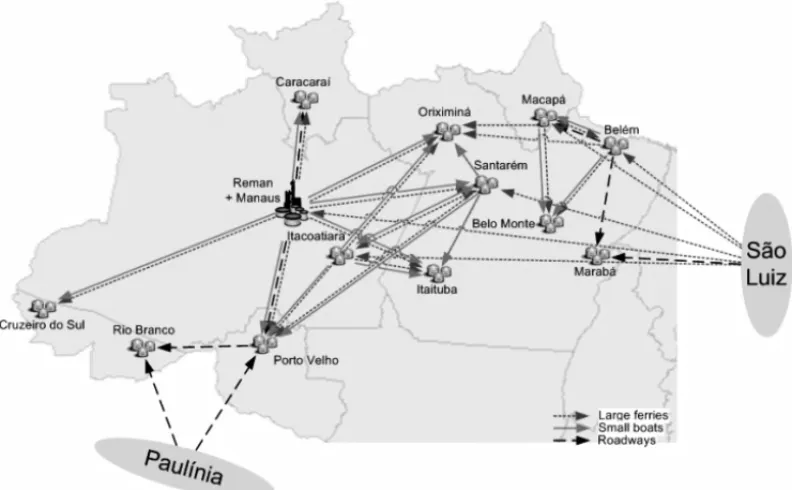
In this section we describe numerical experiments using the proposed methodology for solving a realistic supply chain investment planning under demand uncertainty. The transport in the case study considered is primarily done using waterway modals, which are strongly affected by seasonality issues regarding the navigability of rivers. Four different products were considered – diesel, gasoline, aviation fuel and fuel oil – to be distributed over 19 locations (13 bases, 3 of which have sea terminals, one refinery and two external supply locations).
Figure 1 schematically represents the network under study. The region considered comprises approximately 3.7 MMkm2, which represents nearly 43% of Brazil’s national territory. As shown in this figure, the bases of Manaus (AM), Itacoatiara (AM), Santar´em (PA), Macap´a (AP) and Bel´em (PA) are particularly relevant because they act also as distribution points of the supply coming from S˜ao Luiz (MA).
Waterway transportation is typically done by large ferries during periods of river flooding and by smaller boats during droughts,i.e., in periods of low water levels, the later having higher trans-portation costs. The portfolio of projects considered for the study consists of 28 local projects and 3 arc projects. Such projects are considered mutually independent and can therefore be com-bined as needed by the problem. The planning horizon considered was 8 years, divided into a total of 32 quarters.
To take into account the uncertainty in demand levels for petroleum products, scenarios were generated by the following first-order autoregressive model:
Dtj p=Dtj p−1[1+ωp+σ ε] (24)
where ωP represents the expected average growth rate for the consumption of product p over
the planning horizon, σ represents the estimated maximum deviation for product consumption in the region and ε ∼ N(0,1). The maximum deviation was estimated based on the analysis of the annual consumption historical series over the last 40 years. Each scenario corresponds to a series of demand forecasts for every location and product. The number of scenarios to be used is determined based on a statistical method (Shapiro & Homem-de-Mello, 1998) to obtain solutions within specific confidence intervals for a desired level of accuracy. We use this method as a means of reducing the number of scenarios given that we are sampling from a continuous limited space. For further details on the scenario generation method and definition of sample sizes for this problem, please refer to Oliveira & Hamacher (2012).
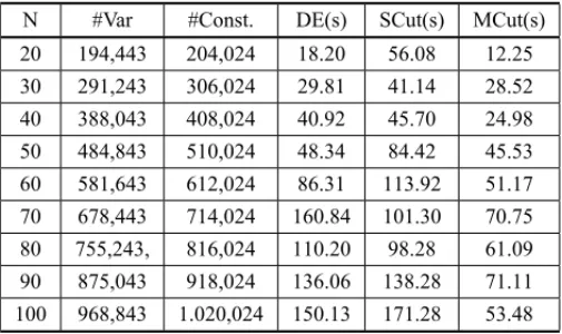
The mathematical model and the scenario generation routines were implemented using AIMMS 3.10. The mathematical model was solved using CPLEX 11.2. All experiments were performed on a Pentium Quad-Core 2.6 GHz with 8 Gb RAM. In AIMMS, an optimality parameter can be specified to decide whether to find the optimal solution or to quickly obtain a suboptimal solution, referred to as aǫ-optimal solution. In these experiments, the execution of AIMMS was stopped when the value of the objective function was within 0.5% of the optimal solution, which is a reasonable choice in terms of solution accuracy. In addition, a time limit of 1 h (3600 s) was set. For the decomposition procedures, the toleranceǫwas equivalently set asǫ=0.005(U B−L B), which is equivalent to define a 0.5% optimality tolerance. Table 1 summarizes the data of the experiments performed.
We solved this case study with sample sizes up to 100 scenarios. For the sample with 100 scenarios, the objective function of the stochastic problem is $73,512.9 million. The solution of the deterministic problem considering the average demand levels for the same 100 scenarios is the suboptimal solution value of $69,714.3 million. The Value of Stochastic Solution (Birge & Louveaux, 1998) for this scenario sample is thus $3,952.6 million, which represents savings of about 5.2%. Table 1 shows the first stage solution for two different sample sizes, namely
Table 1– First-stage solutions.
Project N=20 N=100
Investment period Investment period
Tank – Manaus – Aviation Fuel 9 5
Tank – Santarem – Diesel – 16
Tank – Santarem – Gasoline 24 19
Tank – Santarem – Fuel Oil 1 1
Tank – Bel´em – Diesel 29 24
Pipeline – Macap´a-Santar´em – 15
The first column of Table 2 represents the 9 different instances generated, with 20 up to 100 scenarios. The next two columns summarize the size of the complete model considering all scenarios at once, what is commonly known as the deterministic equivalent (Birge & Louveaux, 1997). It is worth to notice that all instances have the same number of integer variables, a total of 840 each.
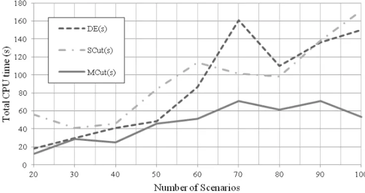
The last three columns from Table 2 show the solving time taken by each technique to reach the ǫ-optimal solution, namely solving the complete deterministic equivalent (DE), using the classical decomposition framework (SCut), and using the proposed multi cut approach (MCut). Figure 2 presents a graphical comparison among the three experiments regarding the CPU time required to reach the optimal solution.
Table 2– Experiment summary.
N #Var #Const. DE(s) SCut(s) MCut(s)
20 194,443 204,024 18.20 56.08 12.25
30 291,243 306,024 29.81 41.14 28.52
40 388,043 408,024 40.92 45.70 24.98
50 484,843 510,024 48.34 84.42 45.53
60 581,643 612,024 86.31 113.92 51.17
70 678,443 714,024 160.84 101.30 70.75
80 755,243, 816,024 110.20 98.28 61.09
90 875,043 918,024 136.06 138.28 71.11
100 968,843 1.020,024 150.13 171.28 53.48
Figure 2– Comparison of computation times.
7 CONCLUSIONS
This paper presents the application of a decomposition scheme for the problem of supply chain design applied to the petroleum byproducts supply chain. We propose a mathematical model that captures the impact of uncertainty on investment decisions, since the problem approached here is a mixture of logistic infrastructure investment planning problem and the stochastic transportation problem. With demand at each destination as a random variable, the objective is to minimize the sum of expected holding and shortage costs, transportation costs, fixed investment costs, and demand shortfall costs.
In order to solve the proposed model, we propose an application of the stochastic Benders de-composition method to the problem also considering the multi cut extension of it, firstly proposed by Birge & Louveaux (1988).
The results suggest that the first approach performs worse than the second in terms of computa-tional time. It is an expected, yet important, result that corroborates the theoretical bounds for the total number of necessary iterations before complete convergence of the algorithms. In a general sense, the multi cut framework performs better than simply solving the deterministic equivalent – or even than directly applying the classic primal decomposition framework – allowing one to solve instances of greater size and, thus, with a more precise representation of the random variables.
ACKNOWLEDGMENTS
REFERENCES
[1] AL-OTHMANWBE, LABABIDIH, ALATIQIIM & AL-SHAYJIK. 2008. Supply chain optimization
of petroleum organization under uncertainty in market demands and prices. European Journal of Operational Research,189(3): 822–840. ISSN 0377-2217.
[2] BEAMONBM. 1998. Supply chain design and analysis: Models and methods.International journal
of production economics,55(3):281–294. ISSN 0925-5273.
[3] BENDERS JF. 1962. Partitioning procedures for solving mixed-variables programming problems.
Numerische Mathematik,4(1): 238–252. ISSN 0029-599X.
[4] BIRGEJR & LOUVEAUXF. 1997. Introduction to stochastic programming. Springer Verlag.
[5] BIRGEJR & LOUVEAUXFV. 1988. A multicut algorithm for two-stage stochastic linear programs.
European Journal of Operational Research,34(3): 384–392. ISSN 0377-2217.
[6] CAIX, MCKINNEYDC & LASDONLS. 2001. Piece-by-piece approach to solving large nonlinear
water resources management models.Journal of Water Resources Planning and Management,127: 363.
[7] CORDEAUJF, SOUMISF & DESROSIERSJ. 2000. A Benders decomposition approach for the
loco-motive and car assignment problem.Transportation Science,34(2): 133–149.
[8] CORDEAU JF, STOJKOVIC G, SOUMIS F & DESROSIERS J. 2001. Benders decomposition for
simultaneous aircraft routing and crew scheduling.Transportation science,35(4): 375.
[9] COSTAAM, CORDEAUJF, GENDRONB & LAPORTEG. 2012. Accelerating benders decomposi-tion with heuristicmaster problem soludecomposi-tions.Pesquisa Operacional,32(1): 03–20.
[10] DEMPSTERMAH, PEDRONNH, MEDOVAEA, SCOTTJE & SEMBOSA. 2000. Planning logistics operations in the oil industry.The Journal of the Operational Research Society,51(11): 1271–1288. ISSN 0160-5682.
[11] ESCUDERO LF, QUINTANA FJ & SALMERON J. 1999. CORO, a modeling and an algorithmic framework for oil supply, transformation and distribution optimization under uncertainty.European Journal of Operational Research,114(3): 638–656. ISSN 0377-2217.
[12] FRANCAPM & LUNAHPL. 1982. Solving stochastic transportation-location problems by general-ized Benders decomposition.Transportation Science,16(2): 113.
[13] GEOFFRIONAM & GRAVES GW. 1974. Multicommodity distribution system design by Benders decomposition.Management science,20(5): 822–844. ISSN 0025-1909.
[14] KHORCS, ELKAMELA, PONNAMBALAMK & DOUGLAS PL. 2008. Two-stage stochastic pro-gramming with fixed recourse via scenario planning with economic and operational risk management for petroleum refinery planning under uncertainty.Chemical Engineering and Processing: Process Intensification,47(9-10): 1744–1764. ISSN 0255-2701.
[15] MAGNANTITL, MIREAULTP & WONGRT. 1986. Tailoring Benders decomposition for uncapaci-tated network design.Netflow at Pisa, pages 112–154.
[17] OLIVEIRAF & HAMACHERS. 2012. Optimization of the Petroleum Product Supply Chain under Uncertainty: A Case Study in Northern Brazil.Ind. Eng. Chem. Res.,51(11): 4279–4287.
[18] SAHINIDISNV. 2004. Optimization under uncertainty: state-of-the-art and opportunities.Computers & Chemical Engineering,28(6-7): 971–983. ISSN 0098-1354.
[19] SHAPIROA & HOMEM-DE-MELLO T. 1998. A simulation-based approach to two-stage stochastic programming with recourse.Mathematical Programming,81(3), 301–325.
[20] VANSLYKERM & WETS R. 1969. L-shaped linear programs with applications to optimal control and stochastic programming.SIAM Journal on Applied Mathematics,17(4): 638–663. ISSN 0036-1399.