UNIVERSIDADE DE
L
ISBOA
Faculdade de Ciˆencias
Departamento de Inform´atica
RESILIENT MIDDLEWARE
FOR A MULTI-ROBOT TEAM
Eric Emmanuel Pascal Vial
MESTRADO EM INFORM ´
ATICA
UNIVERSIDADE DE
L
ISBOA
Faculdade de Ciˆencias
Departamento de Inform´atica
RESILIENT MIDDLEWARE
FOR A MULTI-ROBOT TEAM
Eric Emmanuel Pascal Vial
PROJECTO
Projecto orientado pelo Prof. Doutor M´ario Jo˜ao Barata Calha
MESTRADO EM INFORM ´
ATICA
Thanks
I would like to thank M´ario Calha for all his help and comprehension along these months. A special thank as well to FCT and LASIGE people for their useful support.
Resumo
Actualmente, equipas de robˆos m´oveis intervˆem em diversos contextos e ambientes onde a intervenc¸˜ao humana ´e perigosa ou mesmo imposs´ıvel, podemos mencionar como exemplo a vigilˆancia de espac¸os f´ısicos, como zonas militares ou nucleares. Devido `a crescente complexidade inserida nos seus sistemas, esses robˆos ficam mais poderosos mas paradoxalmente mais suscept´ıveis a falhas de hardware e software. Al´em disso, a incerteza na comunicac¸˜ao wireless pode priv´a-los temporariamente do seu suporte de informac¸˜ao remoto. Este tipo de problema pode ser causado pelo alcance limitado do emissor wireless e pelas zonas de sombra criadas pelo terreno. Por todas essas raz˜oes, desenhar arquitecturas capazes de oferecer mais resiliˆencia para controlo das aplicac¸˜oes, tornou-se um verdadeiro desafio. Este documento aborda um motor cooperativo e re-siliente para equipas de robˆos que lhes permite partilharem uma vista comum e lidar com novos eventos de uma forma fi´avel e resiliente. Este middleware tem como func¸˜ao estab-elecer a guarda de uma qualquer zona f´ısica e detectar eventos inabituais como os intrusos. Neste ultimo caso, um robˆo tem que encontrar uma maneira de bloquear o intruso para o impedir de fugir. O sistema apoia-se em duas caracter´ısticas chave, a primeira ´e uma camada de controlo baseado em dois sub-m´odulos de controlo, o payload e o wormhole, a segunda ´e uma arquitectura baseada em eventos que executam tarefas do payload. Em relac¸˜ao `a camada de controlo, o payload pode ser complexo e acede `a informac¸˜ao partil-hada pelos robˆos enquanto que o wormhole ´e confi´avel mas apenas utiliza a informac¸˜ao local. O payload utiliza uma estrutura de dados chamada “promessa” na qual fornece o deadline correspondente ao momento mais tarde onde deve enviar a pr´oxima promessa. No caso de receber esta promessa depois do deadline, o wormhole considera que o pay-load falhou, toma o controlo e executa as tarefas criticas no lugar do paypay-load. Os eventos s˜ao propagados `as traves de uma estrutura em forma de alvor, da raiz at´e as folhas. Cada folha do alvor ´e um modulo que pode ser executado e produz eventos. A produc¸˜ao dos eventos no alvor pode ser assimilado a uma reacc¸˜ao em cadeia. Durante o ciclo dos even-tos as traves do alvor n˜ao s˜ao poss´ıveis, o que permite evitar as reacc¸˜oes n˜ao controladas e garantem assim a estabilidade do sistema. A juntar a essa arquitectura, propomos tamb´em neste documento alguns mecanismos de sincronizac¸˜oes resilientes, para manter uma vista coerente num mundo ou de navegac¸˜ao para dar ao robˆo a possibilidade de se mover no mundo e de encontrar o melhor caminho. Guardar uma vista homog´enea do mundo ´e um
ponto fundamental que pode n˜ao ser f´acil em caso de uma reuni˜ao de dois grupos. In-troduzimos trˆes implementac¸˜oes de middleware, uma vers˜ao simulada usada para validar arquitectura e testar a sincronizac¸˜ao dos algoritmos num ambiente multi-robˆo, uma vers˜ao m´ovel apontada para ser implementado em plataformas de hardware compostas por robˆos m´oveis reais e finalmente uma vers˜ao de posic¸˜ao capaz de comunicar com robˆos m´oveis, recolher informac¸˜ao e enviar ordens remotas.
Palavras-chave:Middleware, communicac¸˜ao de grupo, robˆos m´oveis, sincronizac¸˜ao de vista
Abstract
Nowadays, teams of mobile robots are involved in many contexts and environments where human intervention would be risky or even impossible, we can mention the surveil-lance of physical areas as military zones or nuclear plants. Due to increasing complexity in their embedded systems, these robots become more powerful but paradoxically more susceptible to face a hardware or software failure. What’s more, unreliability in the wire-less communication could deprive them temporally of their remote information support. For all these reasons, designing architectures able to offer more resilience to the con-trol application has become a real challenge. In this document, we present a middleware architecture for the robots to share a common view and to handle new events in a safe and resilient way. The system relies on two key features, first a control layer based on two sub-modules, the payload and the wormhole, and secondly a cycle-proof event-based architecture used to run critical tasks in the payload. Regarding the control layer, the payload could be complex and has access to information shared among robots, while the wormhole is reliable but only uses local information. The wormhole controls the timely execution of the critical tasks by the payload. In case of timing failure, the wormhole takes control and runs these tasks in place of the payload. In addition to this architecture, we propose as well in this document some resilient synchronization mechanisms to maintain a coherent view of the world when two groups of robots are merging. We introduce three implementations of the middleware, a simulation version used to validate the architecture and test the synchronization algorithms in a multi-robot environment, a mobile version aimed to be ported to hardware platforms composed by real mobile robots and finally a station version able to communicate with mobiles, collect information and send remote orders.
Contents
Figure list xvi
Table list xix
1 Introduction 1
2 Related work and background 3
2.1 Wormhole and payload model . . . 3
2.2 Modules and levels of competence . . . 4
2.3 Group and world view . . . 5
2.4 Localization and navigation . . . 6
2.4.1 World model . . . 7
2.4.2 Wavefront-based algorithm . . . 7
2.5 JNI and multi-thread model . . . 9
3 Design 11 3.1 Architecture overview . . . 11
3.1.1 Wormhole and payload model . . . 11
3.1.2 Tree-oriented architecture . . . 14
3.2 View and group management . . . 17
3.2.1 Time synchronization . . . 17
3.2.2 World view synchronization . . . 18
3.3 World model and navigation . . . 23
3.4 Multi-thread environment and JVM . . . 25
4 Implementation 27 4.1 Middleware versions . . . 27
4.1.1 Simulation version . . . 28
4.1.2 Mobile version . . . 29
4.1.3 Station version . . . 30
4.2 Task management in wormhole . . . 32
4.3 Task and event management in payload . . . 32 xi
4.3.1 Event handling cycle . . . 33
4.3.2 Event and task priority . . . 34
4.4 World view . . . 34
4.4.1 Robot modes . . . 35
4.4.2 World view update . . . 36
4.5 Module tree architecture . . . 36
4.5.1 Communication modules . . . 37
4.5.2 Self-coordination modules . . . 40
4.5.3 Remote control module . . . 42
4.6 Thread concurrency . . . 42
4.7 Programming issues . . . 44
4.7.1 JNI Callback references . . . 44
4.7.2 Avoiding deadlocks between Java and C . . . 46
4.7.3 Memory alignment . . . 47
5 Results and review 49 5.1 Tests and results . . . 49
5.1.1 Blocking movements . . . 49 5.1.2 Payload killing . . . 50 5.1.3 System stress . . . 51 5.1.4 Time synchronization . . . 51 5.2 Work review . . . 52 6 Conclusion 55 A User and developper guide 57 A.1 Linux vs Windows . . . 57
A.2 Sun JDK and Java 3d installation . . . 57
A.3 Eclipse’s configuration . . . 58
A.4 Middleware execution . . . 60
Appendices 56
Glossary 65
Bibliography 68
List of Figures
2.1 Payload and Wormhole layers . . . 4
2.2 Brooks finite state machine . . . 5
2.3 Group merging phase . . . 6
2.4 Example of robot cell assignments . . . 7
2.5 Wavefront-based algorithm . . . 8
2.6 JNI architecture . . . 9
3.1 Middleware layer division and module tree . . . 12
3.2 Wormhole logical flowchart . . . 13
3.3 First example of control change . . . 14
3.4 Second example of control change . . . 14
3.5 Propagation of a produced event . . . 15
3.6 Example of event broadcast with two robots . . . 16
3.7 Two-group synchronization without failure . . . 21
3.8 Two-group synchronization with failure . . . 22
3.9 Three-group synchronization without failure . . . 23
3.10 Example of cell divisions cells . . . 23
3.11 Improved wavefront-based algorithm . . . 24
4.1 Middleware versions . . . 29
4.2 Architecture of the simulation version . . . 30
4.3 Architecture of the mobile version . . . 31
4.4 Architecture of the station version . . . 31
4.5 Event handling cycle . . . 33
4.6 Queue and priority management . . . 34
4.7 Middleware module tree . . . 38
4.8 Communication modules . . . 39
4.9 Updater module flowchart . . . 40
4.10 Navigation modules . . . 41
4.11 Robot heading adjustment . . . 42
4.12 Native function invocations . . . 46
4.13 Deadlock risk between C and Java . . . 47 xv
5.1 Example of blocking movements . . . 50
A.1 JRE setup in Eclipse . . . 58
A.2 Conversion to C Make Project . . . 59
A.3 Native library path . . . 60
A.4 External JAR library path . . . 60
A.5 Auto-build option selection . . . 61
A.6 Filter creation . . . 61
A.7 Global and local world maps . . . 62
List of Tables
3.1 Propagation wave behaviours . . . 24 4.1 Simulation UDP channels . . . 30 4.2 Object attributes . . . 35
Chapter 1
Introduction
Mobile robot teams have the potential to reduce the need of human presence for complex or repetitive tasks. For most of them, the use of cooperation between robots can enhance the overall performance of the team. Achieving an efficient cooperation requires the use of complex algorithms implemented in each robot. This internal complexity in addition to the interaction issue with the environment makes the robot control system more sensi-tive to failures. Nowadays, building resilient control systems for mobile robots is a real challenge.
In this document, we present a middleware architecture for robots in charge of mon-itoring a physical area. In particular, we focus on some architecture features which im-prove the system resilience: A control layer based on two sub-modules the payload and the wormhole which guarantees a timely execution of critical tasks, a event-based archi-tecture in charge of running the payload tasks and which avoids the event cycles, some synchronization mechanisms tolerant to communication failures and used to maintain a common world view for all robots especially during group merging or splitting phases and finally a dual multi-thread environment (Java and C) which communicates through
JNI.
The project context is a cooperative surveillance application of a given area. The cov-ered zone is a campus, a plant or any well-defined area. We assume that the world ground is flat and that each robot follows two-way routes defined in a prior map loaded at the robot startup. The surveillance aims to detect an accident or an intrusion and build a com-mon strategy to handle properly the detected event (e.g. blocking the intruder). All robots run the same version of the middleware and are equipped with sensors, actuators and wireless devices. These devices can be hard connected to the robot or simulated through a simulation environment.
In chapter 2, we introduce some existing concepts and mechanisms we used to design 1
Chapter 1. Introduction 2
the middleware. In chapter 3, we start by presenting the middleware architecture and more precisely the control layer based on the wormhole and payload. Chapter 4 addresses the task and event management and gives a focus on the module tree. In chapter 5, we discuss some test scenarios and provide a short review of the work. Finally, section 6 concludes the document.
Chapter 2
Related work and background
Robot group management covers several areas of techniques. In this chapter, we introduce concepts as the wormhole/payload model or the module-based approach which are key features of the middleware architecture. In section 2.3, group and view management highlights the necessity for the robot to maintain an up-to-date view of the world. The next section presents techniques to enhance the robot ability to navigate in the world. Finally in section 2.5, we describe some programming mechanisms implemented in the middleware.
2.1
Wormhole and payload model
In the vehicular domain, designing safety-critical application is essential, the work in [8], [2] or [10] presents a hybrid (synchronous and asynchronous) control model used in real-time applications. This model is based on two sub-systems, the payload in charge of running complex algorithms to figure out the best behaviour of each car to avoid collisions while the second sub-system, the wormhole is running synchronous and robust algorithms aimed to check whether the payload timely sends corrections to the car actuators. In case a timely timing failure is detected, the wormhole can temporally take control of the car. This technique is applicable to any domain where a safety-critical control is mandatory.
On robots, some critical tasks like the collision avoidance require for the control layer to timely send commands to the hardware layer. Algorithms used to figure out these com-mands might not be deterministic and their computation time may vary especially if they require network communication. The wormhole could check whether these commands are timely sent by the control layer which assumes the role of payload. If so, the wormhole will just forward them to the hardware layer. Otherwise, it will assume the robot’s con-trol by calculating and sending itself these commands. In this latter case, the wormhole would use a low-level algorithm which only involves local information. The wormhole will keep the control until the payload starts again to send commands on time. If the
Chapter 2. Related work and background 4
payload does not regain stability or even no longer sends any command (the payload may
have crashed), the wormhole can restart the whole payload process.
The payload sends the new commands in a structure called the promise. Each promise includes a deadline which enables the wormhole to control the payload’s timeliness. For each promise, the payload is expected to send the next command before the current dead-line is exceeded. The wormhole relies on three modules as shown in figure 2.1: The
Timely Timing Failure Detection (TTFD) monitors the timeliness of the asynchronous payload process and can activate the Safety task to assume control. The Control task
re-ceives the promise which includes the new command and decides whether this command can be forwarded to the actuator layer. The TTFD sends as well control updates to the
payload to inform it won back or lost the control. Ideally, the payload should use these
control updates to improve its performance. In particular, it could try to real-time adjust the priority of some internal processes.
Figure 2.1: Payload and Wormhole layers
2.2
Modules and levels of competence
At the beginning of the 80’s, Rodney A. Brooks [1] developed his subsumption theory based on levels of competence for robots. A lowest level of competence corresponds to a basic robot behaviour. The next levels define more complex behaviours but include the earlier levels of competence. According to Brooks, the key idea is to build a layer-based control system where each layer corresponds to a level of competence. To improve the overall competence of the system and move to the next higher level, we must add a new layer to the existing set.
Chapter 2. Related work and background 5
Each control layer is composed by asynchronous modules which can be seen as finite state machines. As depicted in figure 2.2, the module has input and output signals. Each signal can be modified by a mechanism of suppressor and inhibitor which is based on the signal coming from another module. Some modules can work in closed loops, and thus use as input the feedback signal of other modules.
Figure 2.2: Brooks finite state machine
The idea to break down the control layer into various chains of small modules is powerful. However, it could lead quickly to complex architectures with a huge number of modules. As the information can circulate in cycles, the challenge is to keep the system stable and to avoid an out-of-control propagation of signals.
2.3
Group and world view
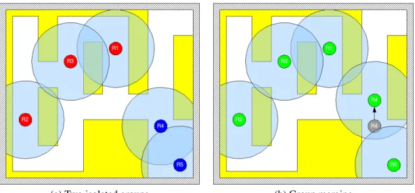
A group so called team is composed by robots which are part of the same network. They can communicate with each other and share information. A group is usually identified by a single id. The figure 2.3a shows two groups of robots with their network range. In figure 2.3b, the move of robot 4 leads to the union of both groups which become a single team.
The world view can be seen as the robot memory. The robot keeps information trans-mitted by its teammates or obtained by its local sources. The view is composed by a list of objects shared by all teammates.
Robot soccer game is an entertaining and well-known application of robot team co-operation. Actually, it shows many common points with our project like the need for all robots to real-time maintain a common view of the world. In the paper [9], the authors present an approach of view model which was successfully implemented during the 2002 RoboCup Sony competition. Due to some high latency in wireless communication, the
Chapter 2. Related work and background 6
(a) Two isolated groups (b) Group merging
Figure 2.3: Group merging phase
robot team does not perform any view synchronization. In order to track a dynamic ob-ject like the ball, each robot combines local information from vision sensors with shared information sent by team-mates. The robot maintains timestamps and uncertainty values for each view object, uncertainty is updated when receiving new information and grows with time.
This type of algorithm could be very efficient in high dynamic environment. However, it is based on a greedy approach in which each robot takes the most reliable information it has. Different robots can make different decisions which could become an issue as we want to build a common strategy for all robots. The other approach relies on a world view synchronization. The system maintains a shared view identical for all robots. The synchronization phase is performed when two robot groups are merging.
2.4
Localization and navigation
In the last twenty years, there has been a considerable amount of work to study mobile robot localization. Researches have been carried out focussing on two problems: com-puting absolute location using a priori map [7] or building incrementally this map while exploring the environment [3]. Both approaches most often rely on complex and math-oriented algorithms based on Kalman filters and maximum likelihood estimation [5]. The present document does not address this kind of problem and we assume that the robot is equipped with a localization device based for instance on GPS or RSS technologies. Given that the robot is able to locate itself in the real world, we have to find the most appropriate world model and the way to make the robot navigate through this model.
Chapter 2. Related work and background 7
2.4.1
World model
There are two kinds of world models, either graph or cell decomposition. The second representation has many variants (adaptive cells, quadtree grid), the most simple is the regular grid based on a cell division. Each cell is a square representing a single world item. All cells have the same dimension. This world item can be a path section, a wall or an obstacle. The main advantage of such a representation is its simplicity and easy implementation. A world map can be coded in a text file where each character represents a cell.
For many calculations, a robot must be assigned to a given cell of the world model ac-cording to its real position in the world, this position is returned by the hardware devices. If we assume that the robot follows a path, the nearest path cell to the robot’s current po-sition is used to assign the cell. Since the robot could have drifted away from its path and given the lack of accuracy of the positioning device, the algorithm can use a maximum error margin. In figure 2.4a and 2.4b, cell assignment is achieved with respectively a low and high margin. In figure 2.4c, cell assignment failed due to a too large margin.
(a) Successful assignment (b) Successful assignment (c) Failed assignment
Figure 2.4: Example of robot cell assignments
2.4.2
Wavefront-based algorithm
The way a robot team performs the surveillance of a physical area could obey many rules in order to maximize the probability of locating an intruder [6]. However, a simple strat-egy could be to make the robot just wander around the world and make random decisions to turn left or right at every crossing. But when a robot needs to meet another robot or block an intruder, some algorithms to calculate the better path are required. Wavefront-based path algorithms are well-suited for grid representations. In this type of algorithm, the wave is propagated from the start point towards all directions until get to the goal cell. The rules are the following:
Chapter 2. Related work and background 8
1. Label all cells with +∞ for the path sections and -1 for the other ones. Label the start cell with 0.
2. For every cell adjacent to the current cell, label it with an increment of the current cell distance if this new value is lower than both current distances of the adjacent cell and goal cell.
3. Continue the propagation from all cells which were updated during the previous step. Stop the algorithm when no more cells are updated.
(a) Iteration 3 (b) Iteration 9
(c) Iteration 11 (d) Gradient descent
Chapter 2. Related work and background 9
Figure 2.5a shows an example of wave propagation with 3 iterations. In figure 2.5b, the descendant wave is stopped because of the distance of the red-circled cell (9). The propagation terminates in figure 2.5c, the distance of the last updated cells is equal to the goal distance (11).
Once the goal cell labelled with the best distance, we have to extract the best path using a gradient descent. First, given label of goal cell as “x”, we find the neighbouring grid cell labelled “x-1” then we mark it as a waypoint. We continue until get to the start cell labelled 0. Figure 2.5d shows the final extracted path. In order to decrease the algorithm convergence time, dual wavefront propagation can be used from both start and goal locations.
2.5
JNI and multi-thread model
The Java Native Interface (JNI) enables the integration of code written in the Java pro-gramming language with code written in other languages such as C and C++. As the reader can find an abundance of basic examples, we will rather focus on the multi-thread issue which is more difficult to deal with. The figure 2.6 shows the interaction between Java and C codes. There are two types of functions implementing the JNI mechanisms: The C native functions called from the Java code and the Java callback methods called from the C code. Java and C codes use multi-thread environments which have to be com-patible each other. That’s why the choice of the multi-thread model is essential.
Chapter 2. Related work and background 10
Running various concurrent threads in the native C library requires to implement mu-tual exclusion mechanisms to avoid the simultaneous access to common resources. Actu-ally, there are two different ways to address this issue in a native C code:
• Create some java.lang.Thread objects and use existing JNI mutex functions like
MonitorEnter and MonitorExit to enter and exit from mutual exclusion zones.
• Use native thread creation and synchronization primitives like the Posix thread li-brary. The mutual exclusion mechanisms are independent from JNI.
The first option is the safest one because we only use a single thread model which is the Java one. That way, we prevent from any compatibility issue between both thread models. The problem is that the C code becomes fully dependant of the Java implemen-tation. Porting this C program to another platform requires to re-write large parts of the original code.
Chapter 3
Design
We start by a description of two main features of the middleware architecture: The
worm-hole/payload model and the tree-oriented architecture. Then sections 3.2 and 3.3
intro-duce mechanisms and algorithms to respectively maintain a coherent shared view between robots and figure out the best path in the world. Finally, the last chapter discusses the multi-thread model and JVM choices.
3.1
Architecture overview
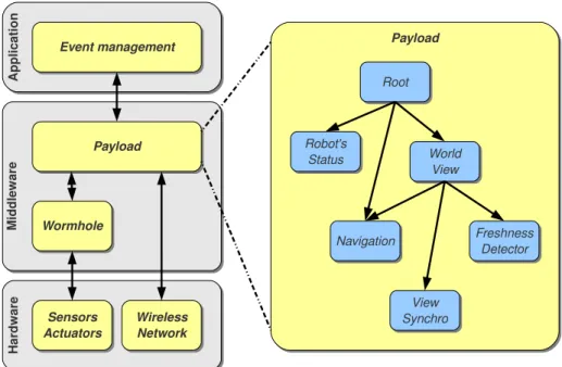
An architecture overview is depicted in figure 3.1. The left side shows the middleware layer division. The wormhole and payload are the middleware basic components. The
wormhole is placed in cut-through configuration between the payload and the
sensor/ac-tuator layer and does not have access to the network device. The payload runs all complex tasks in charge of the robot control. All tasks are triggered by events broadcasted through a module tree. An example of module tree used in the payload is shown in the right side of the figure. Each group of modules is dedicated to a specific task: Position update, navigation or world view management.
3.1.1
Wormhole and payload model
In a first version of the project, a special task (watchdog) was in charge of monitoring the critical tasks running in the middleware. Each task was supposed to be achieved before a given deadline, the latter was calculated in the same way for all tasks. The watchdog real-time monitored a critical task pool. All tasks that real-timed out were considered as blocked and were cancelled then restarted by the watchdog. Although this mechanism is pretty simple, it has many limitations:
• The cancellation success may depend on the task state. This point is particularly true when using some multi-thread implementations as pthreads. A pthread can only be cancelled when blocked in a cancellation point.
Chapter 3. Design 12
Figure 3.1: Middleware layer division and module tree
• The watchdog runs concurrently to the other tasks and thus could be affected in the same way (concurrency issue, computation delay, crash).
• The watchdog just cancels and restarts the task. When restarted, the task may redo some work and put the system in an incoherent state. Moreover, the task may fail once again and lead to a cancellation/restart cycle.
For these reasons, the watchdog approach was not suitable. We needed a more robust and flexible control mechanism which could run in an autonomous way and be placed in cut-through configuration between the critical task and the hardware layer. That way, this control module should be able to ignore a critical task result and take control in place of it which is exactly what the wormhole/payload model does.
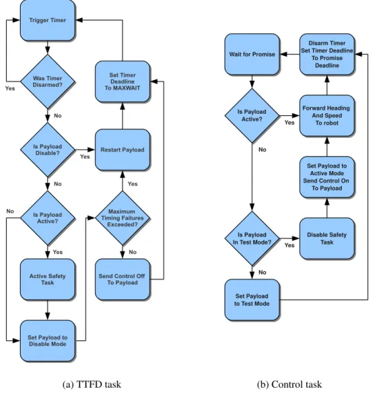
Logical flowcharts of the TTFD and Control tasks are given in figure 3.2. The payload runs in three modes: “active” when it has the control, “disable” when it loses the control after the latest deadline is exceeded and finally in “test”, when the wormhole receives a timely promise while the payload is disabled. The test mode is a transition period, the
wormhole keeps the control and waits for the payload to meet the current deadline before
giving him back control.
There are two restart conditions for the payload. After setting it to disable, the TTFD task will increment a timing failure counter and will wait MAXWAIT milliseconds. If the failure counter is greater than a prior threshold or if no promise is received within this waiting period, the TTFD task will restart the payload. The timing failure counter is
Chapter 3. Design 13
(a) TTFD task (b) Control task
Figure 3.2: Wormhole logical flowchart
reinitialized when the payload wins back control. This counter allows to restart the
pay-load after a given number of failures occurred in a raw but we can imagine more restart
conditions as for instance, a maximum number of failures in a given period of time.
Let’s see now an example of promises exchange between payload and wormhole. In figure 3.3, a first promise gets to the wormhole with a deadline t1. The second promise with deadline t2 is sent timely to the wormhole before t1, the payload keeps the control. At t2, the wormhole has not received yet the next promise so it takes control and sends a control-off acknowledgement to the payload which is disabled. When the promise with deadline t3 gets to the wormhole, the latter keeps the control and set the payload to the
test mode. Finally, the wormhole receives the deadline t4 on time, so it gives control back
Chapter 3. Design 14
Figure 3.3: First example of control change
Figure 3.4: Second example of control change
In the example 3.4, we assume that the payload crashes after sending the second promise. At t1, the wormhole which has not received the new promise, takes control. After MAXWAIT milliseconds, the wormhole considers that the payload is on trouble and restarts it. The rest is similar to the previous example, the wormhole keeps the control until the payload fulfils its new promise with the deadline t2.
3.1.2
Tree-oriented architecture
The event-based architecture is well adapted to robot management. It allows to design a flexible and modular architecture. Indeed, we can create an event type for any robot feature and dedicate a part of the tree to handle this event. Moreover, robot hardware is composed by sensors, actuators and communication devices, each one of them can gen-erate a special event or be triggered by this event. The obstacle event is an example of event which contains the distance values read from the local sensor.
This architecture is a simplified application of the subsumption theory developed by Rodney A. Brooks. The payload is composed by modules and groups of modules, all
Chapter 3. Design 15
gathered in a tree. Each of them is in charge of managing a robot feature. A module can be seen as a process, with a short computation time, which is started by a single incoming event and can produce one or more outgoing events. The number of produced events de-pends on the computation result. All modules could be meshed as a graph and thus make event cycles possible. In order to avoid hazardous out-of-control cycles inside one robot or between several robots, we chose a tree-oriented module architecture.
The tree branch is composed by a group module which is the branch’s root and some child modules (leaf or group) connected under the root. Unlike a leaf module, a group module does not have any computation stuff. Each module can have one or several par-ents. A leaf module computation is started if the incoming event can be consumed by the module. When a leaf module is triggered by a incoming event, the possible outgoing event is broadcasted from the module’s parent which first broadcasted the incoming event.
Figure 3.5: Propagation of a produced event
This mechanism is illustrated in figure 3.5: Group A is parent of Group C, Leaf 1 and
Leaf 2. Group B is parent of Leaf 1, Leaf 2 and Group D. When the red incoming event
triggers the computation of Leaf 1, the green outgoing event is propagated to Group C and
Leaf 2 but not Group D which is not a son of Group A. Group C will keep on broadcasting
the event to its sons and so on. That way, each event is top-down broadcasted until the tree leaves. Three types of events can trigger a module execution:
• Hard events: They are signals generated by the robot’s hardware, e.g. the robot’s clock (beat event) or a distance sensor measure (obstacle event). Such events are always broadcasted from the tree’s root.
• Local soft events: These events are produced by a module and are broadcasted through the neighbour branches (modules with same parent) and the sub-branches. Any module can produce several soft events during the same computation.
• Remote soft events: Instead of being broadcasted locally, they are transmitted through the wireless network and sent to all other robots. Once delivered to a given
Chapter 3. Design 16
robot, the event is broadcasted from the same branch as if it would be produced locally. This mechanism relies on two architecture properties: The module tree has the same structure for all robots which means that any path in the local tree matches the same path in a remote tree. Secondly, the path to locate the module which produced the event in the tree, is stored in the transmitted event. That way, we cannot have event cycles between robots and the remote soft events meet the same constraints as the hard and local soft events.
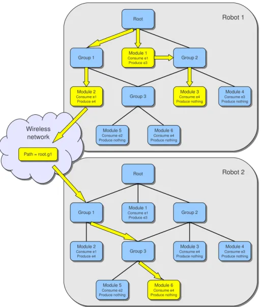
Figure 3.6: Example of event broadcast with two robots
Let’s consider a group of two robots with the same module tree as depicted in figure 3.6. We assume that e1 and e2 are hard events, e3 a local soft event and e4 a remote soft event. Now, let’s have a look on the started modules (in yellow in the figure) if e1 is triggered on robot 1:
Chapter 3. Design 17
• Module 2 of Robot 1 (locally triggered by e1) • Module 4 of Robot 1 (locally triggered by e3)
• Module 6 of Robot 2 (remotely triggered by e4 with path root.g1.
Although module 3 can consume the e4 event, this module is not started in robots 2 because it cannot be reached from the path root.g1. As a leaf module cannot start a computation and produce an outgoing event without incoming event, a cycle of event pro-duction is a chain reaction which always starts with a hard event.
What’s more, this architecture opens the possibility of dynamically enabling or dis-abling a sub-branch of the module tree. When disabled, events are no longer broadcasted through this branch. The activation or disactivation can be performed by any computation module. In our project, each robot has three working modes: Wandering, Searching and
Blocking (an intruder), each mode corresponds to a single branch of the navigation
sub-tree. We use the branch enabling/disabling mechanism to activate the modules associated to the robot current mode.
3.2
View and group management
Given that robots can move away from each other and go beyond their wireless range, a group can be split in various sub-groups. The unreliability of the wireless network can also lead to isolate a single robot if it temporarily loses the Wi-Fi signal. As discussed in section 2.3, the synchronization of all views in this situation is not mandatory, robots could keep on exchanging information and acting according to their local knowledge of the world. But one purpose of the middleware is to provide a cooperative framework to allow robots to build common strategies. This last point implies for all robots to maintain a shared view of the world so a synchronization mechanism is necessary to consolidate the information of each group view especially when two group are merging. This mechanism involves a leader in each group, which is the robot with the lowest id in the group.
3.2.1
Time synchronization
In order to maintain an up-to-date world view, information requires to be timestamped. When an object is transmitted through the network, this timestamp is set by the sender just before the emission. The receiver to make use of the timestamp, must have its internal clock synchronized with the sender or know the time-lag between its clock and the sender one.
Chapter 3. Design 18
As the first solution implies to use dedicated network protocols as NTP to synchronize all clocks, we chose the second solution. But instead of storing as many time-lags as teammates, the robot just maintains one time-lag with its leader. The algorithm 1 details the Object Receiver module involved in the time synchronization phase (line 1). This module is triggered by an Object event received through the network. If the object comes from the leader, the algorithm calculates a mean time-lag over a number of rounds (line 9). The greater is the number of rounds and the more accurate is the time-lag calculation. If the leader has changed since the last iteration, the mean time-lag calculation is re-initialized (line 5). The readTimestamp function (line 12) is used to read an adjusted timestamp value. The robot state parameters are as follows:
• myLastLeader: Latest leader id the time synchronization was performed with. • myRoundNumber: Number of rounds since the time synchronization initialization. • myLagSum: Consolidated time-lag over myRoundN umber rounds.
Algorithm 1Time synchronization algorithm
1: upon event <object| type, id, ts> do
2: if type = ”robot”∧ id = myLeader then
3: delta← DIFFTIME(ts)
4: if id6= myLastLeader then
5: myLastLeader← id
6: myLagSum← delta
7: myRoundN umber← 1
8: else if myRoundN umber < M axRoundN umber then
9: myLagSum← myLagSum + delta
10: myRoundN umber← myRoundNumber + 1 11:
12: functionREADTIMESTAMP(ts)
13: lag ← myLagSum ÷ myRoundNumber
14: return ts− lag
The time synchronization algorithm is very simple. However, the time-lag must be re-calculated at every leader change. As there is no synchronization between teammates, a robot could have started a calculation with the new leader while another robot would still use the time-lag of the old leader. During this short period of time, the timestamp calculated by a robot might be wrong which is not problematic in our case.
3.2.2
World view synchronization
We will now describe in details the synchronization algorithm used to maintain in each robot a coherent world view when two or more groups are merging. This view is
com-Chapter 3. Design 19
posed by all dynamic objects present in the world. The first part will deal with the algo-rithm principles and the second part will present some synchronization scenarios.
Algorithm principles
When two groups are merging, the synchronization is performed by exchanging a synchro event which contains the list of all view objects except for the robots position. This latter is already exchanged through the hello events so including this information in a synchro event would be redundant. The synchro event is normally sent by the group leader. The
synchro event reception is not centralized by the leader, each robot from the destination
group, will handle the synchro event and extract the object list. The synchronization phase ends when all robots have the same leader and group id.
The basic steps below are associated to a faultless synchronization phase. By fault, we mean any event reception failure due for instance to a temporally Wi-Fi signal loss. Different fault scenarios will be discussed in the next section. Two synchro events are exchanged during a faultless synchronization, the first synchro event is always generated by the group leader with the higher id.
• Step 1: Leader 1 receives a hello event from the group leader 2. • Step 2: Leader 1 broadcasts a synchro event through the group 2.
• Step 3: Robots from group 2 receive the object list and update their view. • Step 4: Leader 2 broadcasts a synchro event through the group 1.
• Step 5: Robots from group 1 receive the object list and update their view.
The algorithm 2 gives the modules involved in the synchronization phase. The Hello
Receiver module (line 1) is triggered by an object event which is used by a robot to
broadcast its own position, the module checks out whether this event comes from another leader. The View Synchronizer module (line 9) is triggered by a synchro event, it extracts the object list and updates the local world view (line 16). Finally, the Freshness Detector module (line 22) is triggered by the beat event and removes out-of-date objects from the robot’s view. The beat is a hard event periodically generated by the system. The robot state parameters are as follows:
• myId: single robot identifier.
• myView: view objects including team-mate positions. • myLeader: current group leader identifier.
Chapter 3. Design 20
Algorithm 2View synchronization algorithm
1: upon event <object| type, id, leader, group> do
2: if type = ”robot”∧ (leader 6= myLeader ∨ group 6= myGroup) then
3: if id = leader∧ myId = myLeader ∧ id < myId then
4: SYNCHRONIZATION(myLeader, leader)
5: else if id = myLeader then
6: SYNCHRONIZATION(myId, leader) 7: myLeader← myId
8:
9: upon event <synchro| leader1, leader2, objList> do
10: if myLeader = leader2 then
11: if leader1 < myLeader then
12: myLeader← leader1
13: if myId = myLeader then
14: SYNCHRONIZATION(myId, leader1) 15: for all obj∈ objList do
16: trigger <object| obj.type, obj.id, obj.leader, obj.group>
17: if leader1 > leader2 then
18: myGroup← leader1
19: else
20: myGroup← leader2 21:
22: upon event <beat| > do
23: updateRequired← false
24: for all obj∈ view do
25: if isU ptodate(obj) = f alse then
26: view← myV iew − {obj}
27: if obj.type = ”robot”∧(obj.id = myLeader ∨obj.id = myGroup) then
28: updateRequired← true
29: if updateRequired = true then
30: updateLeader()
31:
32: procedureSYNCHRONIZATION(leader1, leader2)
33: objList← {}
34: for all obj∈ myV iew do
35: if obj.type6= ”robot” then
36: objList← objList + {obj}
37: trigger <synchro| leader1, leader2, objList>
38:
39: procedureUPDATELEADER 40: myLeader← myId
41: myGroup← myId
42: for all obj∈ myV iew do
43: if obj.type = ”robot”∧ obj.id < myLeader then
44: myLeader← obj.id
45: if obj.type = ”robot”∧ obj.id > myGroup then
Chapter 3. Design 21
Examples of synchronization scenarios
The normal synchronization phase is shown in figure 3.7 while figures 3.8 and 3.9 show various synchronization scenarios with respectively two and three different groups merg-ing at the same time. Each group is first composed by two robots. Arrows identify events (blue for hello and red for synchro events) which are handled by robots for the synchro-nization phase. Other hello events broadcasted to periodically announce robot positions are not represented here. Each scenario is given as an example. Therefore, the number of events exchanged during a scenario could be different according to the order each event is delivered with. This statement is especially true if the number of groups merging at the same time is large.
Figure 3.7: Two-group synchronization without failure
In a robot time line, couple of black values correspond respectively to the leader and group id. The hello event parameters are the source robot, leader and group id. Finally, the synchro event parameters are the source and destination leader id (leader1 and leader2 in the algorithm 2).
Scenarios 3.8a, 3.8b and 3.8c highlight temporally reception failures which lead the robot to broadcast extra events to achieve the synchronization. Such failures could be due to a temporary Wi-Fi signal loss. The extra event phase is initialized by the faulty robot which receives a hello packet from its leader. This mechanism is implemented at line 5 of the algorithm 2.
The last scenario 3.9, three groups merging at the same time, is unusual but shows the algorithm resilience. We can notice that at the end of the first “round”, the robot 3 does not have the same group id than the others (yellow-circled value). The situation gets stable after the second hello event.
Chapter 3. Design 22
(a) Reception failure on robot 1
(b) Reception failure on robot 0
(c) Reception failure on robot 3
Figure 3.8: Two-group synchronization with failure
This algorithm is very simple and offers resilience in signal loss situations. Never-theless in some tricky scenarios, it could require more than one round, i.e. more than one hello event to stabilize itself. Hello events are periodically generated (according to the beat signal frequency), so increasing this beat signal frequency to accelerate the syn-chronization phase could be attractive but may on the other hand overload the wireless network and what’s more, lead to some algorithm instability if this frequency is greater than half the mean round trip delay of the wireless network.
Chapter 3. Design 23
Figure 3.9: Three-group synchronization without failure
3.3
World model and navigation
We choose a simple world representation based on a regular grid (see 2.4.1). The real world is divided into regular cells, each cell represents a world item (wall, path, robot, invader). We approximately size the cell to the robot width and assume that an one-cell path does not allow two robots to pass each other (figure 3.10a). The path has to be duplicated to allow two robots to pass one another (figure 3.10b). The path is a special cell used to tag the routes the robots can take in the world. An intruder or any unusual event like a fire, larger than a cell can be split into various cells (figure 3.10c).
(a) One-cell path (b) Two-cell path (c) Large intruder zone
Figure 3.10: Example of cell divisions cells
Regarding the shortest path algorithm, the wavefront-based mechanism described in section 2.4.2 is simple and efficient, however it does not take into consideration the pos-sible obstacles which could block the robot and force it to turn back especially inside an one-cell path. Table 3.1 classifies the obstacles into four categories. We propose an improved version of the algorithm in which each obstacle can affect the behaviour of the propagation wave.
Chapter 3. Design 24
Obstacle type Behaviour
Intruder Stops the propagation wave
Stopped robot Stops the propagation wave
Robot moving in the same direction as the prop-agation wave
Lets the propagation wave go Robot moving in another direction Stops the propagation wave
Table 3.1: Propagation wave behaviours
Let’s consider a world with three robots: R1, R2 and R3. Figure 3.11a shows the path covered by the propagation wave if R1 has stopped, R2 is going up in the same direction as the wave and R3 is going left in the opposite direction to the wave. Unlike R1 and R3,
R2 lets the wave go, the shortest path is given in figure 3.11b after a gradient descent.
(a) Iteration 19 (b) Gradient descent
Figure 3.11: Improved wavefront-based algorithm
As robot moves can change quickly, the shortest path algorithm is computed each time the robot passes through a new cell, until it gets to the goal cell. That way, the shortest path will be updated in case another robot crosses the path or changes its direction.
Another improvement could be to associate a cost to every path cell. This cost could be set according to the ground nature (low cost for smooth ground, high cost for rocky area) and consequently to the robot’s maximum speed on this ground. It could be as well associated with the distance from a identified danger like a fire. The cost would be introduced in the shortest path calculation.
Chapter 3. Design 25
3.4
Multi-thread environment and JVM
As we explained in 2.5, the choice of the multi-thread model is essential. We chose the
pthread library because we wanted the middleware to be as independent as possible from
Java and fully portable to another platform. Regarding the simulation and station versions, the multi-thread model used in the Java virtual machine (JVM) must be compatible with the C multi-thread model. Manipulating native threads in the middleware kernel could lead to deadlocks and crashes if the JVM implementation does not fully support a thread model that matches the native model.
Although we do not notice any crash with Open JDK which is supplied by default with many Linux distributions, this JVM version is said not to be compatible with pthreads. For these reasons, we adopted Sun JDK 6.0 which uses internally pthreads. Moreover this framework is associated with the Java 3D package used in Simbad.
Chapter 4
Implementation
The chapter starts with a presentation of the three implementations of the middleware kernel. For each of them, we will present the interaction between the wormhole and the other layers. The two next sections deal with the task management respectively in the
wormhole and payload. Section 4.4 focusses on the world view content and the update
context. In the next section, we explore the module tree and detail the communication and navigation modules. In section 4.6, we describe some of the mechanisms we used to manage concurrency in both Java and C codes. Finally, in the last section, we address some programming issues we faced during development.
4.1
Middleware versions
The development of the middleware kernel is a large part of this project. The kernel con-tains the wormhole and payload modules and all the event-based architecture we defined previously. The kernel is designed to run in an autonomous way. Three types of interfaces are defined with the robot environment. For each of them, the kernel uses primitives to interact with the real or simulated environment.
• The actuators: The kernel can change the speed and heading of the robot.
• The sensors: The kernel can get the absolute Cartesian position of the robot, as well as its current speed and heading. Moreover, the kernel can read the absolute Cartesian coordinates of an obstacle situated in front of the robot.
• The network: The kernel can send and receive information through a wireless device. That way, it can exchange information with all teammates.
In a real environment, installing such interfaces is not a simple thing and may requires to set up intermediate equipments. In this project, we just assume that the kernel has access to this information. At this stage, we can now present the three versions of the middleware, each one involves one or various kernels:
Chapter 4. Implementation 28
• Simulation: It uses a robot simulation tool called Simbad which allows to easily create a 3D environment with several robots. A robot can be moved around the world using simple Java primitives. For each robot, the simulation runs a differ-ent kernel and simulates the wireless network to exchange information between all robots.
• Mobile: It runs a single middleware kernel and aims to be installed on a hardware platform with hard devices (actuators, sensors, network). The mobile can commu-nicate with others mobiles or stations through the wireless network. This version is fully autonomous.
• Station: It is similar to the mobile as it uses a single kernel. The station runs on a fixed PC and can communicate as well with mobiles or other stations. A Java interface allows to simulate the interaction with the sensors and that way, create fake intruders. Finally, the station can send and receive control events which allow it to remotely control mobiles and collect information. This feature will be detailed further in this chapter.
In simulation and station versions, parts of the code are written in Java. Communica-tion between Java and C codes is handled with the JNI package (Java Native Interface). The figure 4.1 depicts the three combinations of kernels.
The middleware kernel is composed by the wormhole and payload layers. As ex-plained in section 3.1.1, both layers must be as independent as possible. We implemented each one as a single Unix process, the pthread library is in charge of the thread concur-rency management inside a layer. Communication between both wormhole and payload is handled with UDP sockets. The TCP protocol offers a reliable delivery service but is inadequate in wireless environments. We will now enter the kernel architecture and see in details each versions:
4.1.1
Simulation version
Figure 4.2 shows the three simulated JNI interfaces (sensors, actuators and network) which are connected to the wormhole layer. In reality, only the wormhole kernel should compose this layer because the actuators is the only required interface. But maintaining two processes connected with JNI to the Java simulation would not be efficient so the
wormhole sensor and network interfaces are just in charge of forwarding packets to the payload.
The wormhole layer shares three communication channels with the payload each one dedicated to a given type of information: Sensor inputs for channel 1, promises and warn-ing for channel 2 and finally networks events for channel 3. Each channel is handled
Chapter 4. Implementation 29
Figure 4.1: Middleware versions
with UDP sockets. Every interface corresponds to a thread listening to a given UDP port. All ports are dynamically allocated when wormhole and payload are started up. Let’s remember that the simulation layer will launch as many middleware kernels (wormhole and payload) as simulated robots. Table 4.1 details the data exchanged through the three channels.
Finally, we can notice the presence of a bridge between the sensor interface and the
wormhole kernel. As described in section 3.1.1, the wormhole can take control of the
robot through the safety task. This task has to pilot the robot with a basic navigation algorithm and consequently, needs to get some information from the sensor interface.
4.1.2
Mobile version
The mobile version architecture (see figure 4.3) is quite similar to the simulation. The simulation layer and JNI mechanism have disappeared and have been replaced by the
Chapter 4. Implementation 30
Figure 4.2: Architecture of the simulation version Channel Direction Description
1 To payload Current robot coordinates and possibly obstacle coordinates
1 To wormhole Sensor initialization message sent at payload’s start and after any sensor failure
2 To payload Warning message to inform the payload it won or lose control
2 To wormhole Promise including the deadline and the speed/-heading orders
3 To payload Any events sent by the wormhole 3 To wormhole Any events sent by the payload
Table 4.1: Simulation UDP channels
hardware layer. As the wormhole does not access to the network, the wireless interface is directly connected to the payload. As a consequence, there are only two UDP channels between wormhole and payload.
4.1.3
Station version
The station version architecture (see figure 4.4) is actually a mix between simulation and mobile versions. The sensor and actuator interfaces are simulated and connected to a JNI simulation layer. The Java part contains the implementation of a graphic interface used to create fake sensor information. The network interface is connected to the payload as for the mobile version.
Chapter 4. Implementation 31
Figure 4.3: Architecture of the mobile version
Figure 4.4: Architecture of the station version
There is a fourth communication channel used to transport control events. These special events will be further detailed and are exchanged between mobiles and stations. The station uses control events to send remote orders to mobiles or to receive state ac-knowledgements from them. Control events transit through the network so they are first delivered to the payload. The latter uses the control interface to forward these events until the control manager and the Java interface.
Chapter 4. Implementation 32
4.2
Task management in wormhole
As described in 3.1.1, the wormhole main components are the Control, TTFD and Safety tasks. Each of them corresponds to a concurrent process initialized at the wormhole’s startup. The logical flowchart 3.2 gives the actions of each task.
4.3
Task and event management in payload
In this section, we will focus on the payload and especially the event production. Below a list of different types of events and their production context. According to the type, an event can transport some basic data which can be used by the triggered module.
• Beat (hard event): this event is a pulse with a static frequency (currently 2 Hz). The pulse thread generates the beat event every 500 ms and broadcast it from the tree’s root. This event is used by some leaf modules to perform repetitive and regular tasks.
• Obstacle (hard event): This event is generated as soon as an obstacle is detected in front of a robot. The event is produced as long as the obstacle is detected and at the same frequency as the beat event. The event contains the absolute Cartesian coordinates of the obstacle.
• Object (local and remote soft event): This event is the most important one. As a local soft event, it is used to update the robot local view. As a remote soft event, it is regularly sent by a robot to signal its position (hello events). It is used as well by a robot to broadcast an obstacle position update. The event contains all object information: coordinates, speed and heading. If the object is a robot, the robot id,
group id and leader id are also included.
• Synchro (remote soft event): It is produced during the synchronization phase be-tween two groups (see algorithm 2). Each group leader uses it to send the content of their local view. This content can be seen as a list of concatenated object events. • Move (local soft event): The communication modules use this event to inform the navigation modules that the current robot’s route must be recalculated. A world view update means either that some objects have moved in the world so the current best route might have been changed, or that a new intruder has been detected so a new route to get to this intruder must be found.
• Control (hard and remote soft event): It is used by a station to send remote orders to the mobiles. On the other side, it is used by each mobile to send information (as view update status) to the station. This special event is a remote one because it can
Chapter 4. Implementation 33
be broadcasted through the network but it can also be considered as hard because it is initially produced by the station graphic interface.
4.3.1
Event handling cycle
Figure 4.5 illustrates the production cycle of events which always starts with a hard event production. This first event is pushed into the event queue. Then the event dispatcher process pops it from the event queue and broadcasts it from the root of module tree. Each leaf module triggered by the event in the tree must execute its associated task. The task information (module and incoming event) are pushed into the task queue.
Figure 4.5: Event handling cycle
The task dispatcher pops the task from the task queue and assigns it to an available task process from the pool. This pool is a set of running process in charge of executing a module task. Each single execution can lead to the production of local and remote soft events. A local event will be pushed in the event queue but this time, the module’s path in the tree is also saved in the queue. When this event is handled by the event dispatcher, the broadcast will start from this path in the tree as explained in section 3.1.2. If a remote soft event is produced, the process is similar but the event is first sent through the network to all teammates. When delivered, the event is pushed into the teammate event queue with the same path information as it would be produced locally. The cycle continues as long as the queue and task events are not empty.
Chapter 4. Implementation 34
4.3.2
Event and task priority
As some events are more important than others, we introduce three levels of priority (high, normal and low) in the event handling. These priority levels are used in the event and task queues (see figure 4.6). The event extraction mechanism is very basic: As long as there are some high priority events, they are popped then the turn of the normal priority and finally the low priority. This kind of priority management can lead to starvation issues and should be improved. However, the relative low rate of hard event production (every 500 ms for the beat event) makes a congestion quite improbable.
Figure 4.6: Queue and priority management
The event priority in the event queue is forwarded to the task queue with the same priority level. At this stage of the middleware development, the event priority is set as follows:
• High priority: Set for obstacle events • Low priority: Set for the remote soft events • Normal priority: Set for the rest of the events
The reader might be surprised that the beat event is not set to high priority because it is supposed to be produced at regular and accurate intervals. It’s true but the obstacle event has a higher priority because it could trigger an obstacle avoidance procedure in the robot. Moreover, the payload is not synchronous and a few milliseconds late in the beat event production won’t be serious.
4.4
World view
The view contains information transmitted by its teammates or obtained by its own sen-sors. The view is composed of objects which represent a robot or an intruder. The object attributes are given in table 4.2.
The certain attribute is quite important and is worth to be detailed. The value of this attribute changes in the course of time. When true, the object information has a great
Chapter 4. Implementation 35
Name Description
Type Object’s nature i.e. Robot or Intruder Xcoord, Ycoord Object’s Cartesian coordinates in the world
Heading, Speed Object’s heading and speed values (only available for robots) Certain Boolean indicating whether the information is reliable or not Ts Timestamp of the latest information update
Id Object’s identifier
Table 4.2: Object attributes
probability to be correct at the view reading moment. When false, the information is no longer certain but it is still maintained in the view. Actually, when an object is detected by a robot sensor, the information associated to the object is tagged as certain in the view. Later, the certain attribute is set to false in the following situation:
1. The current age of the information calculated from the timestamp value is greater than a given threshold called CERTAINTY MAX AGE.
2. A robot crossed the latest coordinates of the object and did not detect it at this place, which means most likely that the object has moved.
4.4.1
Robot modes
According to the view content, each robot can run in three different modes:
• Wandering: The world view does not contain any reference to an intruder. The robot just wanders around the world, making random decisions to turn left or right at every corner. The robot speed is constant and equal to WANDERING SPEED. • Searching: The world view contains one or several references to an intruder but no
reference with a certain attribute set to true. The robot will try to locate the intruder and will figure out random destination points around the intruder’s latest coordi-nates. The robot speed is constant and equal to SEARCHING SPEED (greater than
WANDERING SPEED).
• Blocking: The world view contains at least one reference to an intruder with a
certain attribute set to true. The robot will try to block the intruder to prevent him
from running away. The robot will calculate the shortest path to get to the intruder location. The robot speed is constant and equal to BLOCKING SPEED (greater than SEARCHING SPEED).
Chapter 4. Implementation 36
4.4.2
World view update
There are basically two sources for view updates: The robot local sensors and the wireless network. Each time a robot receives an update, it will add the information into the view if it is associated to a new object (e.g. a new intruder detection) or it will update the current view object if the update timestamp is newer than the current one. All update situations are listed hereafter:
• The robot detects an intruder in front of it. After updating its own view, the robot will broadcast the update to its teammates through the network.
• The robot does not detect an intruder which is supposed to be in front of it. After updating its own view, the robot will broadcast the update to its teammates through the network.
• The robot receives an object update through the network coming from a teammate. • The robot receives a set of object updates coming from the leader of another group
(synchro packets) which has just merged with the robot’s group.
• The age of an object is greater than a given threshold. The information is updated or removed from the view.
An object is removed from the view if its age is greater than ROBOT MAX AGE for a robot or ROBOT MAX AGE for an intruder. Both thresholds are different because a robot is supposed to broadcast regularly its position via the hello packets. The non reception of these packets must lead quickly to remove the robot from the view. This robot is not part any longer of the group because it faced a communication issue or passed the group Wi-Fi range.
4.5
Module tree architecture
The whole module tree is depicted in figure 4.7, it can be divided into four subsets of modules, each of them represents a branch of the tree:
• Communication: This subset includes all modules connected with positioning and management of the world view.
• Self-coordination: This part deals with all processes necessary to manage the robot in an autonomous way: mainly the collision avoidance and navigation processes. • Multi-robot coordination: These modules are in charge of planning actions
Chapter 4. Implementation 37
• Remote control: This single module handles the communication between mobile and station versions and allows the station to send remote requests to the mobiles.
Actually, the multi-robot coordination subset is empty. These features have not been implemented yet. A good example is the current procedure to block a detected invader. With the self-coordination modules, the robot finds out the nearest entrance point to get to the invader then it calculates the shortest path and moves to the destination point. With a multi-cooperation, the team could run a “consensus” algorithm in order to split up and cover all available entrances. We will now detail the three sub-branches left:
4.5.1
Communication modules
The communication modules are gathered in figure 4.8. First of all, we can notice that the navigation group is connected to the communication branch. That way, the navigation modules can receive the events produced by the branch. The following modules compose the communication group:
Position freshness detector
As it consumes the beat event, this module is run at regular intervals. The current robot coordinates, speed and heading are regularly sent to the payload and timestamped when delivered. The position freshness detector checks whether this information is up-to-date or in other words the information age is greater or not than POSITION MAX AGE. If so, the module sets the robot’s state to LOST. A lost state makes the robot freeze.
Hello sender
This event consumes as well the beat event and sends at regular intervals its position (coordinates, speed and heading) to all teammates through a remote object event. This event will be consumed by the teammate view updater module. This latter will be further described.
Obstacle analyser
The obstacle event is produced by the sensor interface in presence of an obstacle in front of the robot. The analyser module first ensures the robot is not lost and the obstacle coordinates does not correspond to a wall position. This last verification is made on the basis of the local world map. If both verifications are OK, the module produces a local
object event with a object type set to unknown which means the robot does not know the
Chapter 4. Implementation 38