João B. Gonçalves
[email protected] University of Taubate - UNITAU Department of Electrical Engineering, 12060-440 Taubaté, SP. Brazil
Douglas Eduardo Zampieri
Emeritus Member, ABCM[email protected] State University of Campinas - UNICAMP Faculty of Mechanical Engineering CP. 6122 13083-970 Campinas, SP. Brazil
An Integrated Control for a Biped
Walking Robot
The main objective of this work is to present and discuss some results of an integrated control system for a biped robot machine in the dynamic gait. We divided the integrated control system in two sub-systems: a control of the trajectories for the legs and the Automatic Generator of Trajectory. We designed the Automatic Generator of Trajectory by employing a neural network, which updates online the conditions of trajectory for the trunk, from the evolution of the gait, with the objective to reduce the magnitude of the resultant force and moment. We consider that this scheme is a new and interesting approach to generate online the trajectory for the trunk, giving so reflexes for the biped-walking robot.
Keywords: Biped-walking robot, dynamic gait, center of pressure, zero moment point
Introduction
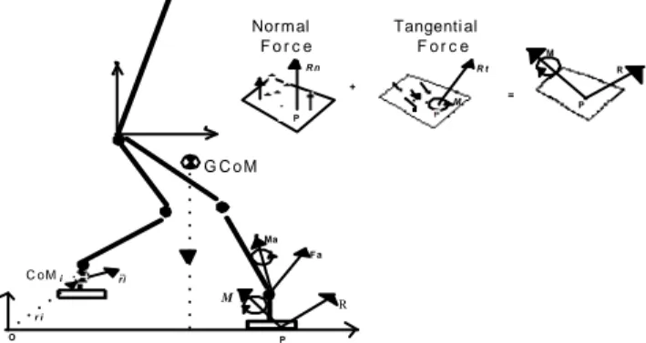
One can classify the biped walking robot by its gait. There are two major research areas in biped walking robot: the static gait and the dynamic gait. When the biped walking robot is in static gait, the ground projection of its global center of mass (GCoM) must be in the foot-support area (support polygon or stability region). In this case, the localization of the center of pressure (CoP) is identical to the GCoM. Otherwise, when the GCoM leaves the support polygon, the biped-walking robot is in dynamic gait; but the CoP always falls within the foot-support area (Goswami, 1999). When the GCoM is in front of the CoP, the distance between themselves can provide a measure of the walking stability, which defines the static threshold of stability. Existing inertial and gravitational forces, this distance adds torques that cause turns around the CoP and the possible fall of the biped walking robot. Figure 1 presents a scheme for this problem.1
M R
i ri..
r i
O
R n
M
+
=
R t
P
P
Ma F a
P
M R
G C o M Nor m al
F o r c e
Tangenti al F o r c e
C oM
Figure 1. Biped walking robot in the dynamic gait.
According Figure 1, one can measure the inertial and gravitational forces for each center of mass of the link, relative to the inertial coordinate system. Resultant force R and moment M are caused because the interaction between the foot-support and the foot-support area, which are applied to the point P (CoP). In addition, one can describe the dynamic of the biped walking robot
Presented at XI DINAME – International Symposium on Dynamic Problems of Mechanics, February 28th - March 4th, 2005, Ouro Preto. MG. Brazil. Paper accepted: June, 2005. Technical Editors: J.R.F. Arruda and D.A. Rade.
using a resultant force Fa and a moment Ma. Therefore, one can guarantee the postural stability of the dynamic gait if the values of the components Fa, Ma, R and M on the foot-support area, are null. In this case, one can identify the point P as zero-moment point (ZMP).
The challenge is to endow the biped walking robot with a trunk (inverted pendulum) and provide a trajectory for the trunk to compensate torques inherent to the dynamic gait. Since the inertial and gravitational forces are considered, the dynamic modeling of the trunk considers the dynamic interaction between the legs and the trunk, establishing a system of non-linear equations whose input is the trajectories of the legs. One can design the trajectories to the legs and then determine the trajectory for the trunk that assures the walking stability (Li, Q. et al., 1992).
Many papers have proposed to assure the dynamic gait for the biped-walking robot, discussing the walking stability, dynamic gait design and dynamic control. Goswami (1999) presented a stability indicator named FRI-point (foot-rotation indicator), which might be restricted to the support polygon. Nevertheless, the FRI-point can leave the support polygon; one can use this distance as a measure of the walking stability.
Typically, one can use the trajectories of the trunk to guarantee the walking stability for the biped-walking robot. In this case, one might design a dynamic gait for the biped-walking robot and, next, compute the trajectories of the trunk by considering the ZMP. One can look for this algorithm in Yamaguchi et al. (1993), Li et al. (1992), Kajita et al. (1991), Takanishi (1989) and Park et al. (1998).
Shibata et al. (2000) proposed a scheme to control a biped-walking robot whose objective is to reduce the magnitude of the resultant force R and moment M by controlling the acceleration of the GCoM. He proved this scheme by considering a biped-walking robot with eight degree-of-freedom, without a trunk. Cheng et al. (1997) proposed a control system based on a genetic algorithm (GA) whose objective was to optimize dynamic gait of the biped-walking robot. The project of the control system and the gait generator to the biped-walking robot were formulated as an optimized problem, and a GA scheme was designed to solve it, using several criteria. Hasegawa et al. (2000) designed a hierarchical control system based on a GA whose objective was to optimize the consumption of energy, by finding a natural gait for the biped-walking robot. They proposed an optimized problem, with constraints to compute the trajectories to the legs that result in a low power consumption by the actuators.
system for a biped walking robot in the dynamic gait. We divided the integrated control system in two sub-systems: a control of the trajectories for the legs and the trunk, based on adaptive control system, and an automatic generator of trajectory (AGT) for the trunk. We designed a AGT by employing a neural network, which updates online the conditions of trajectory for the trunk, from the evolution of the gait, with the objective to reduce the magnitude of the resultant force R and moment M. We considered that the AGT scheme is a new and interesting approach to generate online the trajectory for the trunk, giving reflexes for the biped-walking robot.
Nomenclature
A = Matrix Associated to the Reference State Vector.
A1 = Diagonal Matrix Associated to the
A
Matrix.A2 = Diagonal Matrix Associated to the
A
Matrix. B = Matrix Associated to the Source Vector. bd = Dynamic Friction.bs= Static Friction (Coulomb Friction).
C = Couriolis and Centripetal Forces Vector. D = Matrix Mass.
e = Error Vector.
e = Length of the link, m.
F = Dissipative Force Vector. Fa = Resultant Force Vector, N.
G = Gravitational Force Vector.
g = Gravitational force, Ns2/m. I = Moment of Inertia, kgm2.
M = External Resultant Moment Vector, Nm.
m = Mass of the link, kg.
Ma = Resultant Moment Vector, Nm. P = Center of Pressure.
R = Resultant Force Vector, N. Rn = Normal Force Vector, N.
Rt = Tangential Force Vector, N. sgn(•) = Signal Function.
{
xC yc zc}
= Coordinates of the Center of Mass, m.Greek Symbols
ξ = Damping Factor.
θθθθ = Angular Position Vector, rad. ττττ = External Force Vector. κκκκ = Gain Vector.
ω = Natural Frequency, rad/s.
∆∆∆∆ = Resultant Generalized Force Vector between hip and trunk. γ = Small Positive Parameter.
Ω Ω Ω
Ω = State Vector.
Ω = Reference State Vector.
Γ
∆ˆ = Parametric uncertainties about non-linear term.
Biped Robot Machine
We conceived our prototype of the biped walking robot by using the Solidworks® software (Predabon, E. and Bocchese, C., 2003), whose basic philosophy was to elaborate a three-dimensional prototype, divided in subsystems properly joined to impose the restrictions of the relative movements. The physical parameters (mass, volume, moments of inertia, etc) of the prototype are calculated automatically, from the characteristics of the materials to be used, from the forms, geometric dimensions and coordinate systems.
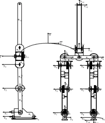
The biped walking robot comprises rigid links (ankles, lower legs, upper legs and hip) interconnected by revolute joints, which constitute the legs. Solidary to the hip there is an inverted pendulum, with two perpendicular revolute joints that allow a three-dimensional pendulum movement. Figure 2 illustrates the biped walking robot. We employed the rules of Denavit-Hartenberg to distribute the Cartesian coordinates systems; in this case, links and joints are marked in a systematic way.
j1 1
z0
x0
y0
y1 z1
x1
z2
x2
y2
z3
x3
x4
y3
y4 x5
y5
x6
z6
x7
z7
x8
z8
y9 x9
y1 0 x1 0
x y
j1
j2
j3
j4
j5
j6
j7
j8
j9
j1 0
z
e0
e1
e2
e3
e4
e5
e1 2
z1 1
x1 1
z1 2
x1 2
e1 1
j1 2
Figure 2. Biped walking robot model.
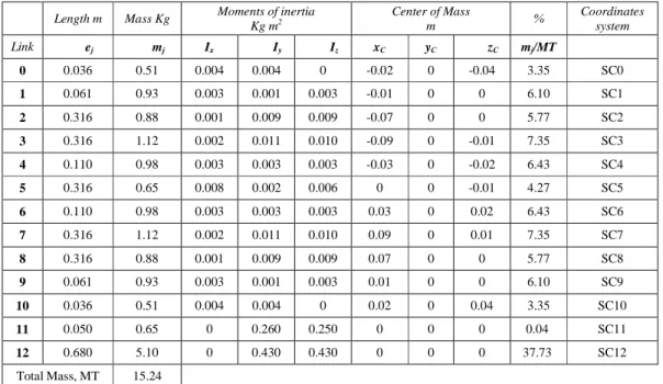
Table 1. The physical parameter of the biped walking robot.
Length m Mass Kg Moments of inertia
Kg m2 Center of Mass m % Coordinates system
Link ej mj Ix Iy Iz xC yC zC mj/MT
0 0.036 0.51 0.004 0.004 0 -0.02 0 -0.04 3.35 SC0
1 0.061 0.93 0.003 0.001 0.003 -0.01 0 0 6.10 SC1
2 0.316 0.88 0.001 0.009 0.009 -0.07 0 0 5.77 SC2
3 0.316 1.12 0.002 0.011 0.010 -0.09 0 -0.01 7.35 SC3
4 0.110 0.98 0.003 0.003 0.003 -0.03 0 -0.02 6.43 SC4
5 0.316 0.65 0.008 0.002 0.006 0 0 -0.01 4.27 SC5
6 0.110 0.98 0.003 0.003 0.003 0.03 0 0.02 6.43 SC6
7 0.316 1.12 0.002 0.011 0.010 0.09 0 0.01 7.35 SC7
8 0.316 0.88 0.001 0.009 0.009 0.07 0 0 5.77 SC8
9 0.061 0.93 0.003 0.001 0.003 0.01 0 0 6.10 SC9
10 0.036 0.51 0.004 0.004 0 0.02 0 0.04 3.35 SC10
11 0.050 0.65 0 0.260 0.250 0 0 0 0.04 SC11
12 0.680 5.10 0 0.430 0.430 0 0 0 37.73 SC12
Total Mass, MT 15.24
Dynamic Model
We considered the biped walking robot as a mechanism in an open chain. By using the formalism of Denavit-Hartenberg to describe its kinematics characteristics, we derived the inverse kinematics and the dynamic modeling. For the dynamic modeling, the software Maple® V (Geddes et al. 1997) was used to implement the formularization of Newton-Euler (Craig, 1995), which permitted the automation of the process of symbolic modeling (acronym NEROBOT). The basic data necessary to use the program NEROBOT are the parameters of Denavit-Hartenberg, the moments of inertia, the mass, and the center of mass of each link. Therefore, the result is a dynamic model in the matrix form, given in Eq. (1).
( )
+( )
+( )
= − −∆+C G F M
Dθɺɺ θɺ,θɺ θ θɺ τ (1)
We considered the biped walking robot as two subsystems: the legs and the trunk (inverted pendulum). The interaction between the subsystems is caused by the generalized forces of reaction in the joint between the trunk and the hip (∆∆∆∆), which is caused by their relative movements. Thus, we admitted that the dynamics of the mounted inverted pendulum on a car in movement represents the main characteristics of coupling between these subsystems.
Using the NEROBOT, we obtained the dynamic model of the legs, presented in the literal form, due to the complexity and the great extension of its model. For simplifications we considered M=0 in Eq. (1), resulting Eq. (2).
( ) ( )
+ +( )
= −∆+ θθ θ θ τ
θ C F G
Dɺɺ ɺ,ɺ ɺ (2)
According Shilling, R. J. (1990), we used the followed friction term:
( )
( )
(
)
− − + + =∆ γ θ θ θθ d j
j s j d j j j v j j
j b b b b
F
ɺ ɺ
ɺ
ɺ sign exp (3)
Equation (3) is composed by a viscous friction bv (coefficient of viscous friction), by a dynamic friction bd and by a static friction bs
(Coulomb friction.) Sign stand for the sign function, and γ is a small positive parameter. If the speed of the biped-walking robot is reduced, the relative effects of static friction become more pronounced, as represented in Eq. (3). Otherwise, if the biped-walking machine speed increases, the viscous friction term becomes larger, in comparison with the other friction terms. According to Eq. (3), we considered the dynamic frictionbd 0.62
j= Ns/m, the static
frictionbs 0.91
j= Ns/m and γ = 0.2.
By using the NEROBOT, one can derive a dynamic model for the trunk, in which, for simplification, we considered M = 0 and F =
0 in Eq. (1), resulting Eq. (4) and Eq. (5).
(
)
( )
(
2)
12 12 12 12 12 5 0 12 11
5+m +m zɺɺ =m e cosθ θɺɺ −θɺ
m (4) = + + + 3 2 3 2 12 11 2 12 12 22 0 0 g g c c I e m d z θ θ ɺ ɺ ɺ ɺ
( )
+ = 5 12 12 12 3 2 cos 0 z em θ oɺɺ
τ τ (5) Where:
( )
[
]
[
( )
]
{
+ + +}
+= cos2 1 cos2 1
2 1 12 12 2 12 12
22 m e θ Iy θ
d
( )
(
11 12)
2 11 3 12 11 12 cos
2m e e +e m +m
+ θ (6)
[
( )
(
2)
12 11 12( )
12]
11 12 1212 12
2 sin2θ m e I 2m e e sinθ θɺ θɺ
c =− + y + (7)
( )
(
)
( )
212 12 12 11 12 2 12 12 12
3 sin2 sin
2
1 θ θ θɺ
+ +
= I m e m e e
c y (8)
( )(
)
( ) ( )
{
e m m m e}
gg2=− 11sinθ11 11+ 12 + 12 12cosθ11 cosθ12 (9)
( ) ( )
ge m
The term 5 0
zɺ
ɺ of the Eq. (4) is an acceleration of the link e5, with respect to the inertial frame SC0. The dynamic of the legs of the biped-walking robot is considered on the left side of Eq. (4); and the generalized force of reaction vector is considered on the right side. We considered the generalized forces of reaction vector as disturbances to the movement of the biped walking robot.
Similarly, the terms on the left and the right side of the Eq. (5) are related to the dynamic of the inverted pendulum and to the generalized forces of reaction vector (which is considered a disturbance to the movement of the inverted pendulum), respectively. Therefore, Eq. (4) and Eq. (5) show the influences of the movements of the dynamic legs in the movement of the inverted pendulum and vice-versa.
Integrated Control System
The integrated control system is considered by two subsystem controls: the first, which uses feedback linearization and adaptive control approach and, the second, which is an automatic generator of trajectories for the trunk. Similarly, to the control of the trajectories of the legs, one can control the trajectories of the trunk by employing the computed torque technique (Craig, 1995) whose control law contains the terms of the nominal model of the robot, the reference model and the uncertainties. Neural networks using radial basis functions (RBF) provide the on-line identification of the uncertainties. The automatic generator of the trajectories for the trunk uses a recurrent neural network (RNN) that manipulates the positions and velocities of the legs to compute the positions for the trunk, based on the zero moment point (ZMP) criterion. Figure 3 illustrates the proposed scheme for the integrated control system.
Figure 3. Scheme for the integrated control system.
Feedback Linearization and the Adaptive Control Approach
Project of the Reference Model
One can consider a second-order reference model, whose locations of the poles in the complex plan agree with the project specifications, so that the servomechanism simulates the analogous behavior of the standard second-order systems (Ge et. al. 1998). This control technique is similar to the supervised learning. The reference model provides the desired patterns (targets) for the input (references trajectories). To adjust the parameters of the compensator and of the model of the plant is used the error between the desired patterns and the measured variables.
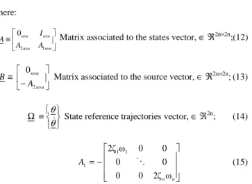
By considering a second-order model for each degree of freedom, Eq. (11) represents the reference model in the state space form.
u B AΩ+ =
Ωɺ (11)
Where: ≡ × × × × n n n n n n n n A A I A 1 2
0 Matrix associated to the states vector, ∈ ℜ2n×2n;(12)
− ≡ × × n n n n A B 2 0
Matrix associated to the source vector, ∈ ℜ2n×2n
; (13) ≡ Ω θ θ
ɺ State reference trajectories vector, ∈ ℜ2n; (14)
− = n n A ω 2ζ 0 0 0 0 0 0 ω 2ζ 1 1
1 ⋱ (15)
Diagonal matrix with n products between ζ (damping factor) e ω (natural frequency)
− = 2 2 1 2 ω 0 0 0 0 0 0 ω n
A ⋱ (16)
Diagonal Matrix with n natural frequency (ω), rad/s; Project of the Adaptive Control System
Equation (17) represents a biped walking robot in the state space form. One can suppress the dependence of the angular variable to simplify the notation.
(
+Γ−∆)
+ Ω =
Ω −1τ
BD A ɺ (17) Where: ≡ × × × × n n n n n n n n I A 0 0 0 (18)
Matrix associated to the state vector, ∈ ℜ2n×2n
≡ × × n n n n I
B 0 Matrix associated to the source vector, ∈ ℜ2n×n; (19)
≡ Ω θ θ
ɺ State vector, ∈ ℜ2n; (20)
(
C+G+F)
− ≡
Γ Non-linear terms of the model of the robot; (21)
By admitting that the uncertainties are null, Equation (22) defines a control law that includes terms of the dynamic model of the robot and the reference model.
[
]
(
+ Ω−Ω)
+∆Using Eq. (16) into (21) results:
[
]
(
A+BA A)
Ω+Bu =Ωɺ 1 2
u B AΩ+ =
Ωɺ (23)
Equation (23) describes a linear, stable and not-connected model. One can define the error of tracking e≡Ω−Ω as the difference between Eq. (23) and Eq. (11), which results:
e A
eɺ= (24)
By analyzing Eq. (24), one can guarantee the asymptotic tracking by an adequate choice of the matrix associated to the state vector for the reference model. However, it is necessary the full knowledge of the dynamics of the plant to be controlled in order to make it possible to cancel the nonlinear effect of the model.
Inclusion of the Parametric Uncertainties
The full knowledge about a dynamic model is not possible in the practical application. Thus, we admitted the parametric uncertainties related to Eq. (21), which does not allow the exact cancellation of this term. One can define ττττM, the term based on the model, and ττττR, the robust term. Thus, according Ge, et al. (1998) Eq. (22) can be changed by Eq. (25), which presents Γ⌢ an estimated of the Eq. (20).
[
]
(
)
( )
R M e A A D u B B D τ τ κτ= −1 + 1 2 Ω−Γˆ +∆+− sgn (25)
Where:
κ Gain vector;
( )
•sgn Signal function; e Error of the model
Using Eq. (17) into Eq. (25), one can write:
[
]
(
+ Ω−Γ+ +Γ)
+ Ω =
Ω − −
R A A D u B B D BD
A 1 2 ˆ τ
1 1
ɺ
Ω=
(
+[
]
)
Ω+ + −1(
+Γ−Γˆ)
21 A Bu BD R
A B
A τ
ɺ (26)
Ω= Ω+ + −1
(
+∆ˆΓ)
R BD u B
A τ
ɺ (27)
The difference between Eq. (27) and Eq. (11) results:
(
Γ)
− +∆
+
= 1 ˆ
R BD e A
eɺ τ (28)
Analyzing Eq. (28), we conclude that the objective of the ττττR term is to suppress the error in the process of identification of the
estimated term∆ˆ . Γ
Equation (29) can give the estimated term vector∆ˆ . In this Γ context, neural network is an interesting way to emulate the unknown terms. In special, we employed a radial base function (RBF) neural network because one can adaptively adjust their weights based on the Lyapunov stability theory, when the radial base function vector is considered fixed (Ge et. al. 1998.) In this paper, we employed for each neuron of the RFB network the inverse Hardy’s multiquadric. Ξ + • = + ≡ ∆ ∆ ∆ = ∆ Γ Γ Γ Γ ρ ρ ρ ρ T T n T T v v v v n 2 1 2 1 n 2 1 ε ε ε ˆ ˆ ˆ ˆ ⋮ ⋮ ⋮ (29)
Where the k-th component is:
[
]
k km 1 k m 1 ε ε ρ ρ v v v 1
ˆ + ≡ +
=
∆Γ v ρ
T k
k ⋯ ⋮ (30)
According to GE et al. (1998), one can rewrite Eq. (28) with Eq. (29) to assure the stability in the Lyapunov sense.
{
}
RT BD BD v BD e A
eɺ= + −1 •ρ + −1Ξ+ −1τ (31)
In addition, one can consider the following Lyapunov function:
( )
= +∑ Π= − n
i i i
T i T v v Pe e e v V 1 1 , (32) Where:
P = PT Solution of the Lyapunov equation:ATP+PA=−Q; (33) Π
Π Π
ΠIConstant matrix definite positive (34)
Taking the time derivative of the Eq. (32) and using Eq. (31) results:
( )
=[
+{
•}
+(
Ξ+)
]
+ ∑ Π= − −
− n
i i i
T i R T T v v BD v BD e A P e v e V 1 1 1 1 2 2 , ɺ
ɺ ρ τ (35)
According to Eq. (35), one can choose Eq. (36) as an adaptability law for the parameters of the RBF net.
1
− Π
−
= e PbD
v i
T i i
i ρ
ɺ (36)
Using Eq. (35) into Eq. (36) results:
( )
(
R)
T T PBD e e A P e v e
V = + −1Ξ+τ
2 2
,
ɺ (37)
Using Eq. (30) and Eq. (33) to rewrite Eq. (37) results:
( )
1(
(
1)
)
sgn 2
,v =−e Qe+ e PBD− Ξ−k e PBD− e
Vɺ T T T
(38)
The matrixes P and B are definite positive and D is a non-singular matrix. One can assure the stability in closed loop by choosing the components of matrix k according to Eq. (39).
i ii
k ≥ ∆ˆΓ (39)
Therefore, Eq. (38) is definite negative:
( )
e,v =−e Qe−2e PBD−1 <0The Automatic Generator Trajectories of the Trunk
Commonly, to compensate the inertial and gravitational forces intrinsic to the dynamic gait, one can endow the biped walking robot with a trunk (inverted pendulum). However, this addition causes inherent problems to the stability. First, we must to keep the trunk under control in the vertical position; we solved this problem by employing a servomechanism as showed in section 4.1. The generation of trajectory of the trunk that can assure postural stability is the second problem. It is worthy to consider the dynamic of the contact between the support foot and the ground. The ZMP criterion can provide a system of nonlinear dynamic equations to obtain the trajectories of the trunk (Takanishi, 1989).
Gonçalves and Zampieri (2003) addressed the second problem by employing a recurrent neural network (RNN) to generate the trajectories of the trunk in the automatic form, based on the ZMP criterion. They designed an identification scheme to obtain the parameters vector of the RNN, utilizing a first-order standard
back-propagation with momentum. This way, a compensative trunk motion makes the actual ZMP get closer to the planned ZMP.
Here, we utilized the same scheme, using an RNN with 2 intermediate layers, and 20 neurons in each layer. The stop criterion was 0.0001 m that is the mean-square error between the actual ZMP and the planned ZMP.
Simulations and Results
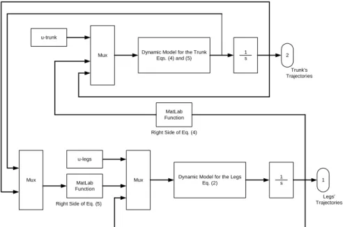
We considered the biped walking robot as two subsystems: trunk (inverted pendulum) and the legs. Equations (2), (4) and (5) define the dynamic model of the biped walking robot. We implemented this model in Matlab/Simulink®, by using the S-functions (Harman, T. L. and Dabney, J. B., 2003.) Figure 4 illustrates the disturbances caused by the trunk in the legs (Right Side of Eq. 4) and vice versa (Right Side of Eq. 5). The connection named "u-trunk" receives the trajectories of the trunk from the generator of trajectories for the trunk. The connection "u-legs" receives the planned gait from the gait automatic generator.
Mux Dynamic Model for the TrunkEqs. (4) and (5) 1s
Mux Dynamic Model for the LegsEq. (2) 1s 1 2
u-trunk
u-legs
Mux MatLab
Function
MatLab Function
Right Side of Eq. (4)
Right Side of Eq. (5)
Trunk's Trajectories
Legs' Trajectories
Figure 4. The biped walking model implementation.
Figure 5 illustrates the integrated control system for the biped walking robot. The block "Biped Robot’s Model" contains the models of the subsystems and the disturbances. The adaptive control systems for the trunk and for the legs, in despite of independent, are
similar. The automatic generator of trajectories for the trunk receives the angular signals of position and acceleration from the gait generator and the trunk, to compose the input signals to the RNN.
Biped Walking Model (Figure 4) Feedback Linearization
and Adaptive Control for the Legs
Feedback Linearization and Adaptive Control
for the Trunk
u-legs
u-trunk Automatic Generator
of Trajectories for the Trunk Off-line Gait Generator
Legs' Trajectories
Trunk's Trajectories
For the simulation, we utilized a dynamic gait with the following characteristics: the pelvis remains parallel in relation to the ground; the step length is 0.17 m; the speed walking is 0.55 m/s; the angle between the foot and the ground is 0.2 rad; and the maximum height for the balancing foot is 0.0386 m. The total time to complete a step is 0.3 s. We considered that twenty percent of the total time is time expended in the bi-support phase.
For this gait characteristic, we computed the angular positions by using inverse kinematics techniques, and the speeds, by employing Jacobian computation.
Figure 5 and Fig. 6 show the results of the simulation, which describe the angular and the velocity trajectories for the first (θ1),
second (θ2), third (θ3) joints, and so on.
Figure 6. Angular position for the legs.
Figure 7. Angular velocities for the legs.
Figure 8 shows the trajectories for the angular position and the velocity of the trunk that were used for the reference of the trunk. The RNN decides the problem of the angular positioning of the trunk and the angular velocities of the trunk are decided from the reference model.
Figure 9 shows the tracking errors obtained from the control system of the trunk. The angular position error is around ± 1.5××××10-3
rad and presents a decreasing oscillatory behavior. The corresponding angular speeds present similar behavior.
Figure 8. Reference signals for the trunk.
Figure 9. Tracking errors for the trunk.
Figures 10 and 11 present the corresponding errors (E =θ -θ
j
j j )
of the tracking of the position and of the velocities associates to the legs, respectively. The angular position errors are limited around
Figure 10. Tracking error of the legs’ position.
Figure 11. Tracking error of the legs’ velocity.
Conclusions and Comments
This work aimed at contributing to the area of biped walking robots that explore the dynamic gait. We designed a biped walking robot endowed with trunk, composed by a chain of rigid links interconnected by rotating joints, totalizing twelve joints that enable positioning in the three-dimensional space. For the symbolic modeling, we implemented the formalism of Newton-Euler in the environment of the Maple®, offering an automatic symbolic modeler.
We projected and implemented the integrated adaptive control system. The control law includes terms of the dynamic model of the robot, of the reference model and of the uncertainties. We employed an RBF neural network for the on-line identification of the parametric uncertainties; and, we design and implement an automatic gait generator, adaptable to the local conditions of the
land, functioning perfectly in terms of passage speed, length of the step and maximum height for the foot in balance. After planning the gait, was determined the trajectory for the trunk by a RNN, integrated to the control system, which could update online the angular positioning of the trunk from the evolution of the legs. The system of control and the automatic generator of trajectories for the trunk constituted the adaptive mechanisms, developed to solve the dynamic gait control.
In the simulation, we synthesized a gait for the robot with requirements similar to those of the human being gait, with a walking speed of 2 km/h. By using the inverse kinematics computation, was computed the corresponding angular position. The angular speeds were computed by using Jacobian matrix, as show in Fig. 6 and Fig. 7.
The integrated control system presents a steady behavior and, besides tracking signals of reference for the legs and for the trunk, allows rejecting the disturbances caused by the coupling between the legs and trunk.
References
Cheng, M.-Y. and Lin, C.-S. Genetic Algorithm for control design of biped locomotion. Journal of robotic system 14(5), 365-373 (1997).
Craig, John J. Introduction to robotics: mechanics and control. Addison-Wesley Longman. 2nd ed, 1995. 450 p.
Ge, S. S., Lee, T. H. and Harris, C. J., 1998, “Adaptive Neural Networks Control of Robotic Manipulator.” World Scientific Series in Robotics and Intelligent Systems, Vol. 19, 381 p.
Geddes, K., Monagan, M. B. and Springer-Velarg, 1997, “Maple V Programming Guide.” Ed. Springer-Verlag NY. 379p.
Gonçalves, J. B. and Zampieri, D. E., 2003, “Recurrent Neural Network Approaches for Biped Walking Robot based on Zero-Moment-Point Criterion.” RBCM - J. of. the Brazilian Soc. Mechanical Sciences, Vol. XXV. pp 53-62.
Goswami, A., 1999, “Postural Stability of Biped Robots and the Foot-Rotation Indicator (FRI) Point”. The International Journal of Robotics Research, Vol. 18, No. 6, pp. 523-533.
Harman, T. and Dabney, J. B., 2003, “Mastering Simulink”. Ed. Prentice-Hall. 400 p.
Hasegawa, Y., Arakawa, T., and Fukuda, T. Trajectory generation for biped locomotion robot. Mechatronics 10 (2000) 67-89. Elsevier Science Ltd.
Kajita, S., and Tani, K. Study of dynamic biped locomotion on rugged terrain: Derivation and application of the linear inverted pendulum mode. Proceedings of the IEEE International Conference on Robotics and Automation. Sacramento, CA. pp. 1405-1411, 1991.
Li, Q., Takanishi, A., and Kato, I., 1992, “Learning Control of Compensative Trunk Motion for Biped Walking Robot based on ZMP criterion.” In Proceedings of the 1992, IEEE/RSJ International Conference on Intelligent Robots and System. Raleigh, NC.
Park, J. H., and Kim K. D. Biped robot walking using gravity-compensated inverted pendulum mode and computed torque control. Proceedings of the IEEE International Conference on Robotics and Automation. Lueven, Belgium. 1998.
Predabon, E. and Bocchese, C., 2003, “SolidWorks 2004 – Projeto e Desenvolvimento”. Ed. Érica. 408 p.
Shibata, M., and Natori, T. Impact Force Reduction for Biped Robot Based on Decoupling COG Control Scheme. IEEE AMC. Nagoya. 2000.
Shilling, R. J., 1990, “Fundamental of Robotics Analysis and Control”, Prentice Hall, 425 p.
Takanishi, A., 1989, “Robot Biped Walking Stabilized with Trunk Motion.” Proceedings of ARW on Robotics and Biological System.