Constraints on the pMSSM, AMSB model and on other models from the search for long-lived charged particles in proton-proton collisions at sqrt(s) = 8 TeV

CERN-PH-EP/2013-037 2015/07/29

CMS-EXO-13-006

Constraints on the pMSSM, AMSB model and on other

models from the search for long-lived charged particles in

proton-proton collisions at

√

s

=

8 TeV

The CMS Collaboration

Abstract

Stringent limits are set on the long-lived lepton-like sector of the phenomenologi-cal minimal supersymmetric standard model (pMSSM) and the anomaly-mediated supersymmetry breaking (AMSB) model. The limits are derived from the results pre-sented in a recent search for long-lived charged particles in proton-proton collisions, based on data collected by the CMS detector at a centre-of-mass energy of 8 TeV at the Large Hadron Collider. In the pMSSM parameter sub-space considered, 95.9% of the points predicting charginos with a lifetime of at least 10 ns are excluded. These constraints on the pMSSM are the first obtained at the LHC. Charginos with a life-time greater than 100 ns and masses up to about 800 GeV in the AMSB model are also excluded. The method described can also be used to set constraints on other models.

Published in the European Physical Journal C as doi:10.1140/epjc/s10052-015-3533-3.

c

2015 CERN for the benefit of the CMS Collaboration. CC-BY-3.0 license

∗_{See Appendix B for the list of collaboration members}

1

Introduction

We present new constraints on long-lived chargino production in the phenomenological min-imal supersymmetric standard model (pMSSM) [1] and on the anomaly-mediated supersym-metry breaking (AMSB) model [2–4]. In the pMSSM, we consider the parameter sub-space for particle masses up to 3 TeV and charginos (χe

±_{) with a mean proper decay length (cτ)greater}

than 50 cm. In the AMSB model, the small mass difference between the lightest chargino and neutralino (χe

0

1) often leads to a long chargino lifetime.

Long-lived charged particles are predicted by various extensions of the standard model (SM) [5– 7], such as supersymmetry (SUSY) [8] and theories with extra dimensions [9, 10]. If such par-ticles have a mass lighter than a few TeV they could be produced by the CERN LHC. The en-ergy available in the proton-proton (pp) collisions at the LHC is such that particles with mass

&100 GeV and lifetime greater than O(1)ns could be observed with the CMS detector [11] as high-momentum tracks with anomalously large rates of energy loss through ionization (dE/dx). These particles could also be highly penetrating such that the fraction reaching the CMS muon system would be sizable. The muon system could therefore be used to help in identification and in the measurement of the time-of-flight (TOF) of the particles. The signature described above is exploited in a previous CMS search [12], which sets the most stringent limits to date on a number of representative models predicting massive long-lived charged particles such as tau sleptons (staus), top squarks, gluinos, and leptons with an electric charge between e/3 and 8e.

The main thrust of this paper is to present constraints on the pMSSM and the AMSB model, obtained using the results from the search for heavy stable charged particles (HSCP) in proton-proton collisions at√s = 7 and 8 TeV [12]. The method applied relies on the factorization of the acceptance in terms of two probabilities, calculated using the standard CMS simulation and reconstruction tools at 8 TeV. Moreover, the results of the acceptance calculations have been tabulated and made publicly available [13]. Thus this technique, which allows the signal acceptance for a model with long-lived particles to be computed using the kinematic proper-ties of the particles at their production point, may in the future be used by others to evaluate constraints on other extensions of the SM without use of the CMS software.

2

The CMS detector

The central feature of the CMS apparatus is a superconducting solenoid of 6 m internal diame-ter providing a field of 3.8 T. Within the field volume are a silicon pixel and strip tracker, a lead tungstate crystal electromagnetic calorimeter, and a brass and scintillator hadron calorimeter. Muons are measured in gas-ionization detectors embedded in the steel flux-return yoke of the magnet. The tracker measures charged particles within the pseudorapidity range|η| <2.5 and provides a transverse momentum pT resolution of about 2.8% for 100 GeV particles. The

ana-log readout of the tracker also enables the particle ionization energy loss to be measured with a resolution of about 5%. Muons are measured in the range|η| < 2.4, with detection planes based on three technologies: drift tubes, cathode strip chambers, and resistive-plate chambers. The muon system extends out to 11 m from the interaction point in the z direction and to 7 m radially. Matching tracks in the muon system to tracks measured in the silicon tracker results in a transverse momentum resolution between 1 and 5%, for pT values up to 1 TeV. The time

resolution of the muon system is of the order of 1 ns. This provides a time-of-flight measure-ment that can be used to determine the inverse of the long-lived particle velocity as a fraction of the velocity of light (1/β) with a resolution of 0.065 over the full η range [12]. A more detailed

2 3 Estimation of signal acceptance

description of the CMS detector, of the coordinate system, and of the kinematic variables can be found in Ref. [11].

The first level of the CMS trigger system, composed of custom hardware processors, uses infor-mation from the calorimeters and muon detectors to select the events of interest. The high-level trigger processor farm further decreases the event rate from around 100 kHz to around 400 Hz for data storage.

3

Estimation of signal acceptance

Transcribing the results presented in Ref. [12], in terms of limits on models other than those considered in the reference, requires the tabulation of the relevant signal acceptance. This ac-ceptance can then be used to constrain the beyond the standard model (BSM) scenarios, as described in the next sections. There can be significant differences in signal acceptance be-tween the models investigated in Ref. [12] and the model to be tested. These differences arise because the dE/dx and TOF measurements are affected by the distribution and orientation of the material encountered by particles travelling within the CMS detector. The combination of these effects with the differences in the kinematic properties between models can result in large differences in signal acceptance.

The signal acceptance can be accurately computed by fully simulating and reconstructing sig-nal events in the CMS detector and by applying the same selection criteria as adopted in Ref. [12]. We refer to this method of determining the signal acceptance as the “full simula-tion”. This procedure requires extensive knowledge of the CMS detector and in particular use of CMS software that accurately models detector response to simulated signal events and em-ploys the full CMS reconstruction routines such that identical selection criteria can be used on simulated signal events as on data collected from collisions.

An alternate method, which only requires information on the kinematic properties of the long-lived particles at their production point, is presented here. Such a method can be used if the efficiency for triggering and selecting events can be expressed in terms of probabilities asso-ciated with each individual long-lived particle. This is the case for models with lepton-like massive long-lived particles since the event selection specified in Ref. [12] imposes only re-quirements on measurements performed on individual particles. The adjective “lepton-like”, defined in Ref. [12], indicates particles that do not interact strongly and are therefore not subject to hadronization.

The event selection requirements of Ref. [12] are expressed in terms of measured pT, dE/dx,

TOF, and mass values of individual particles in an event. The probability that a long-lived par-ticle in an event passes the online or offline selection requirements in Ref. [12] can be expressed as a function of the true (generator-level) kinematic properties (k) of the particle: β, η, and pT.

Any other equivalent set of kinematic and directional variables could also be used to express this dependence. The offline selection of Ref. [12] has fixed values for pT, dE/dx, and TOF

thresholds but uses different reconstructed mass thresholds (m_thresh) depending on the mass (m) of the long-lived particle in the model being tested.

With these individual particle probabilities, the acceptanceAfor a model to pass the online and offline selections can be computed with a Monte Carlo technique by generating a large number of events N such that

A = 1 N N

∑

where Pon(k1_i, k2_i, . . . , kM_i ) is the probability that the event with index i containing M long-lived particles with true kinematic properties k1_i, k2_i, . . . , k_iM passes the online selection, and

Poff(mthresh, k1i, k2i, . . . , kMi ) is the probability that the event with the same kinematic

proper-ties passes the offline selection with mass threshold mthresh, after having passed the online

selection. Given the mass resolution of the detector, a mass threshold of mthresh ' 0.6m has

an efficiency of about 95% for the benchmark models considered in Ref. [12]. Consequently, throughout this paper, mass thresholds of 0, 100, 200, and 300 GeV are used for true long-lived particle masses of m ≤ 166, ≤330, ≤500, and ≥500 GeV, respectively. The choice of 100 GeV steps for the mass thresholds is made so that the information provided in Table 3 of Ref. [12] re-garding the background expectation and the observed count in the signal region may be used, thus allowing a more general application of the factorization method. In the case where only one long-lived particle is present in each event, the probabilities have the simplest form Pon(k)

and Poff(mthresh, k). If each event contains two long-lived particles, the probabilities can be

expressed using the probabilities for events with either single long-lived particle: Pon(k1_i, k2_i) =Pon(k1_i) +Pon(k2_i) −Pon(k_i1)Pon(k2_i);

Poff(m_thresh, k1_i, k2_i) =Poff(m_thresh, k1_i) +Poff(m_thresh, k2_i) −Poff(m_thresh, k1_i)Poff(m_thresh, k2_i). (2)

The expression for events with more than two long-lived particles per event can also be ex-pressed in terms of the probabilities Pon_{(k)and P}off_(m

thresh, k)associated with each individual

long-lived particle.

The probabilities Pon(k)and Poff(mthresh, k), derived using the full simulation as described in

the Appendix, are evaluated using the selection requirements adopted by the “tracker+TOF” analysis described in Ref. [12]. This selection, where tracks are required to be reconstructed in both the tracker and the muon system, has been shown to be the most sensitive to signatures with lepton-like long-lived particles. The probabilities thus obtained are stored in the form of look-up tables.

The factorization method described above is validated by comparing the estimated signal ac-ceptance values with those obtained with full simulation for a few benchmark models predict-ing long-lived leptons. In the rest of this paper we refer to the former as “the fast technique”. In the full simulation case, pileup due to multiple interactions per bunch crossing is also simu-lated. Agreement better than 10% between full simulation and the fast technique presented in this paper is generally observed for the considered values of mthresh.

More details on the determination of the probabilities Pon_{(k)and P}off_(m

thresh, k)can be found

in the Appendix, which also contains the details of the validation of the fast technique based on Eq. (1). The Appendix also explains how this technique can be used in the future to estimate the CMS exclusion limits for extensions of the SM other than the ones considered in this paper using publicly available look-up tables for Pon(k)and Poff(mthresh, k).

The probabilities Pon(k)and Poff(mthresh, k)are computed with simulated stable particles, but

the method is easily extended to particles with finite lifetimes by correcting the Pon_(k)

proba-bility for the probaproba-bility that the long-lived particle, with mass m, lifetime τ, and momentum p, travels at least the distance x required to produce the minimum number of track measure-ments in the CMS muon system, as required in Ref. [12]. The correction consists of an expo-nential factor, exp[−mx/(τ p)], to be applied to Pon(k). This correction is not applied also to

4 3 Estimation of signal acceptance

only depends on the pseudorapidity of the particle:

x=      9.0 m 0.0≤ |η| ≤0.8; 10.0 m 0.8≤ |η| ≤1.1; 11.0 m 1.1≤ |η|. (3)

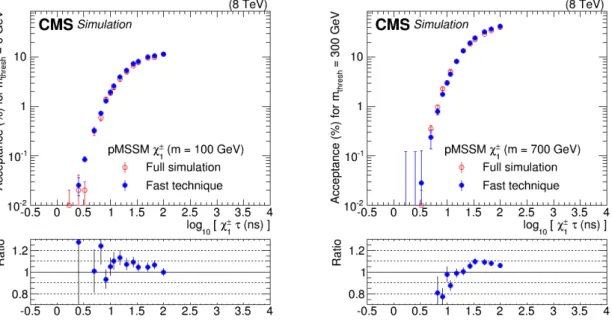
These values of x ensure that the particle traverses the entire muon system before decaying. This choice results in a conservative estimate of the signal acceptance since it ignores the contri-bution to the acceptance from particles that decay before the end of the muon detector but still pass the selection. In Fig. 1, the acceptance obtained with the fast technique is compared with the acceptance obtained with the full simulation of the detector, as a function of the lifetime of the particle. It can be seen from the ratio panels that in most cases the agreement between the two methods is within 10%, corresponding to the systematic uncertainty in the fast estimation technique used to compute the acceptance. For lifetimes less than 10 ns, the spread is somewhat larger, but the tendency to underestimate the acceptance is less than 15%.

Figure 1: Signal acceptance as a function of the chargino lifetime for a benchmark model having a chargino of mass 100 GeV (left) and 700 GeV (right), with a mass threshold of 0 GeV and 300 GeV, respectively. The panel below each figure shows the ratio of acceptance from the fast technique to the acceptance obtained from a full simulation of the detector.

The offline event selection in Ref. [12] includes two isolation requirements. The first is defined by ΣpT < 50 GeV, where the sum is over all tracks (except the candidate track) within a

ra-dius∆R= √(∆η)2_{+ (∆φ)}2 _{=0.3 around the candidate track. The second requirement is that}

E/p<0.3, where E is the sum of energy deposited in the calorimeters within a radius∆R=0.3 around the candidate track (including the candidate energy deposit) and p is the candidate track momentum reconstructed in the tracker. The probabilities Pon(k)and Poff(mthresh, k)are

estimated with single-particle events and thus do not account for the possibility that a long-lived particle might fail the isolation requirements. In order to accurately model the isolation requirements, the following procedure, which uses generator-level information from a sim-ulation of the BSM model under test, should be used. The isolation requirements must be determined for each long-lived particle at the generator-level. The following conditions are

imposed: charged particles ∆R<0.3

∑

∑

The equations (4) represent the generator-level equivalents of the tracker and calorimeter iso-lation requirements, respectively. The sum of the tracks pT around the long-lived candidate is

replaced by a sum over transverse momenta of all charged particles around the direction of the long-lived particle. Similarly, the sum of the calorimeter energy deposits around the long-lived candidate is replaced by a sum over the energies of all visible particles, except the long-lived one, around the direction of the long-lived particle of momentum magnitude p. Muons are not considered in the sum over visible particles since they deposit very little energy in the calor-imeter. If a long-lived particle does not satisfy both isolation requirements expressed by Eqs. (4), the corresponding factor Poff(mthresh, k)in Eq. (2) is set to zero. While pileup effects are not

taken into account in the above prescriptions, it was checked that these omissions do not have a significant effect on the results. The robustness of the fast estimate of the acceptance against the hadronic activity surrounding the long-lived particle is assessed by testing different chargino production mechanisms: direct pair production of charginos, pair production of gluinos that each decay to a heavy quark (b,t) and a chargino, pair production of gluinos that each decay to a light quark (u,d,s,c) and a chargino, and pair production of squarks that each decay to a quark and a chargino. A∼10% agreement between the fast estimate of the model acceptance and the full simulation predictions is observed as shown in Fig. 2. The estimate of the acceptance for chargino pair production is not modified by the isolation requirement since the charginos are always isolated for that production mechanism.

In the two following sections, the fast technique is used to estimate the signal acceptance of the CMS detector for two extensions of the SM. Given that no significant excess of events over the predicted backgrounds is observed in Ref. [12], the signal acceptance estimated with the technique described above is used in calculating cross section limits of these models, at 95% confidence level (CL). The limits in this paper are established using the CLSapproach [14, 15]

where p-values are computed with a hybrid Bayesian-frequentist technique [16]. A log-normal model [17, 18] is adopted for the nuisance parameters. The nuisance parameters are: the ex-pected background in the signal region, the integrated luminosity, and the signal acceptance. The expected background and the integrated luminosity, as well as their uncertainties, are pro-vided in Ref. [12]. The uncertainty in the signal acceptance is assumed to be 25% for all signal models. This value results from adding 10% to the≤15% uncertainty reported in Section 6 of Ref. [12]. The additional 10% accounts for the systematic uncertainty incurred by the use of the fast estimation technique to compute the acceptance. Table 1 summarizes the information needed, in addition to the signal acceptance evaluated with the fast technique, to set limits on a signal model predicting lepton-like charged long-lived particles.

To demonstrate the validity of this procedure, we have used it to translate the estimate of the signal acceptance to the 95% CL limit on the production cross section for two of the models considered in Ref. [12]. The limits obtained on the pair production and inclusive production of staus in the context of the gauge mediated supersymmetry breaking (GMSB) model are shown in Table 2 for signal acceptance values estimated with full simulation and with the procedure described above. The limits obtained with the two techniques agree within 8%. The differences are due only to a small difference in the signal acceptance computed with the two different techniques and to the larger uncertainty assigned to the acceptance from the fast technique. The results in Table 1 may be compared with those shown in Table 7 and Fig. 8 of Ref. [12]. In making the comparisons, it should be noted that there are important differences in the way that

6 3 Estimation of signal acceptance -1 χ + 1 χ g~~g→ tt/bb g~g~→ qq q~q~ = 100 GeV thresh Acceptance (%) for m ₀ 10 20 30 40 50 60 70 80 (stable, m = 200 GeV) ± 1 χ Full simulation Fast technique (w/o iso) Fast technique (with iso)

Ratio 0.8 1 1.2 (8 TeV) CMSSimulation -1 χ + 1 χ g~g~→ tt/bb g~g~→ qq ~q~q = 300 GeV thresh Acceptance (%) for m ₀ 10 20 30 40 50 60 70 80 (stable, m = 700 GeV) ± 1 χ Full simulation Fast technique (w/o iso) Fast technique (with iso)

Ratio 0.8 1 1.2 (8 TeV) CMSSimulation

Figure 2: Signal acceptance as a function of the chargino production mechanism for a bench-mark model having a chargino of mass 200 GeV (left) and 700 GeV (right), with a mass threshold of 100 GeV and 300 GeV, respectively. From left to right, the production mechanisms considered are: direct pair production of charginos; pair production of gluinos that each decay to a heavy quark (b,t) and a chargino; pair production of gluinos that each decay to a light quark (u,d,s,c) and a chargino; and pair production of squarks that each decay to a quark and a chargino. The panel below each figure shows the ratio of acceptance from the fast technique with the isolation requirements to the acceptance obtained from a full simulation of the detector. The estimated acceptance is given with and without the generator-level isolation. Pileup is present only in the full simulation samples.

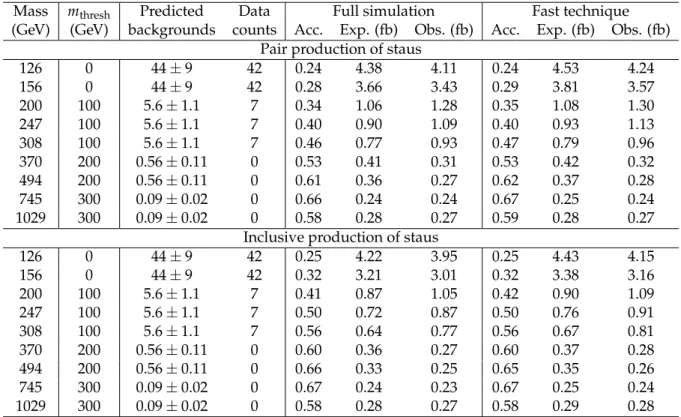
Table 1: Summary of the information needed to set limits on a signal model predicting lepton-like charged long-lived particles. The mass threshold, the corresponding expected background, and the observed numbers of events, as well as the uncertainty in the signal acceptance evalu-ated with the fast technique, are provided as a function of the long-lived particle mass.

Mass mthresh Predicted Data Signal Unc.

(GeV) (GeV) backgrounds counts (%)

m<166 0 44±9 42 25

166<m<330 100 5.6±1.1 7 25 330<m<500 200 0.56±0.11 0 25

500<m 300 0.090±0.02 0 25

m_thresh is chosen in the two cases. In Ref. [12] the value was varied in steps of 10 GeV in order

to optimise the resultant limit. In this paper a simpler approach has been followed with m_thresh varied in 100 GeV steps and chosen to be the largest value satisfying the condition mthresh ≤

0.6m. The latter approach generally results in a somewhat higher estimation of the background and therefore a more conservative limit. In the most extreme case, the pair production of staus, with m= 308 GeV, the background is estimated to be 5.6±1.1 events with mthresh = 100 GeV,

compared with the estimate of 0.7±0.1 events obtained with mthresh = 190 GeV in Ref. [12],

resulting in a cross section limit that is about three times higher in the former case. Nonetheless, the limits agree within∼15% in almost all cases, allowing restrictive limits to be set on a general class of models.

Table 2: Signal acceptance estimated from the fast technique and with the full simulation of the detector, as well as the corresponding expected and observed cross section limits. Results are provided for both the pair production and the inclusive production of staus as predicted by the GMSB model. The mass threshold, the corresponding expected background and the observed numbers of events is also shown.

Mass mthresh Predicted Data Full simulation Fast technique

(GeV) (GeV) backgrounds counts Acc. Exp. (fb) Obs. (fb) Acc. Exp. (fb) Obs. (fb) Pair production of staus

126 0 44 ± 9 42 0.24 4.38 4.11 0.24 4.53 4.24 156 0 44 ± 9 42 0.28 3.66 3.43 0.29 3.81 3.57 200 100 5.6 ± 1.1 7 0.34 1.06 1.28 0.35 1.08 1.30 247 100 5.6 ± 1.1 7 0.40 0.90 1.09 0.40 0.93 1.13 308 100 5.6 ± 1.1 7 0.46 0.77 0.93 0.47 0.79 0.96 370 200 0.56 ± 0.11 0 0.53 0.41 0.31 0.53 0.42 0.32 494 200 0.56 ± 0.11 0 0.61 0.36 0.27 0.62 0.37 0.28 745 300 0.09 ± 0.02 0 0.66 0.24 0.24 0.67 0.25 0.24 1029 300 0.09 ± 0.02 0 0.58 0.28 0.27 0.59 0.28 0.27

Inclusive production of staus

126 0 44 ± 9 42 0.25 4.22 3.95 0.25 4.43 4.15 156 0 44 ± 9 42 0.32 3.21 3.01 0.32 3.38 3.16 200 100 5.6 ± 1.1 7 0.41 0.87 1.05 0.42 0.90 1.09 247 100 5.6 ± 1.1 7 0.50 0.72 0.87 0.50 0.76 0.91 308 100 5.6 ± 1.1 7 0.56 0.64 0.77 0.56 0.67 0.81 370 200 0.56 ± 0.11 0 0.60 0.36 0.27 0.60 0.37 0.28 494 200 0.56 ± 0.11 0 0.66 0.33 0.25 0.65 0.35 0.26 745 300 0.09 ± 0.02 0 0.67 0.24 0.23 0.67 0.25 0.24 1029 300 0.09 ± 0.02 0 0.58 0.28 0.27 0.58 0.29 0.28

Because the online selection in Ref. [12] uses a missing transverse energy (E_Tmiss) trigger in com-bination with a single-muon trigger, there is one caveat to the proposed factorization method: the efficiency of the Emiss_T trigger cannot be modeled accurately in terms of single long-lived particle kinematic properties. Accounting for the presence of other undetectable particles us-ing a Monte Carlo method would not help because Emiss

T often depends significantly on detector

effects due to the other particles. The assumption that the E_Tmisstrigger adds negligibly to the event selection performed by the muon trigger must therefore be satisfied in order to apply the method to a given signal. Deviations from this assumption would result in an underestimation of the signal acceptance. The assumption is satisfied by models with lepton-like long-lived par-ticles. Models with long-lived colored particles, such as top squarks or gluinos, do not satisfy this condition and thus cannot currently be tested with the technique presented in this paper. Long-lived colored particles hadronize in color singlet bound states [19] that could interact with the detector material leading to complex situations, detailed in Refs. [12, 20], and induc-ing significant instrumental Emiss_T . For instance, pair-produced colored long-lived particles may hadronize to a charged and a neutral hadron. In this case the E_Tmissis strongly modified by the presence of the neutral hadron since it is not visible in the tracker and deposits onlyO(1)GeV in the calorimeter. Moreover, the interactions of the color singlet bound states with matter may lead to a modification of the electric charge of the bound states [19]. In this case, the hadron containing a long-lived colored particle can be electrically charged at production, but neutral in the muon system and therefore fail the muon reconstruction. The probabilities Pon(k)and Poff_(m

thresh, k)do not account for the possible modification of the electric charge experienced

8 4 Constraints on the pMSSM

4

Constraints on the pMSSM

The pMSSM is a 19-parameter realization of the minimal supersymmetric model (MSSM) [1] that captures most of the phenomenological features of the R-parity conserving MSSM. The free parameters of the pMSSM, in addition to the SM parameters, are: (1) the gaugino mass parameters M1, M2, and M3; (2) the ratio of the vacuum expectation values of the two Higgs

doublets tan β = v2/v1; (3) the higgsino mass parameter µ and the pseudoscalar Higgs mass

mA; (4) the 10 sfermion mass parameters mFe, where eF = Qe1, eU1, eD1, eL1, eE1, eQ3, eU3, eD3, eL3, eE3

(imposing degeneracy of the first two generations m_Qe

1 ≡ mQe₂, meL₁ ≡ meL₂, . . . ); and 5) the

trilinear couplings At, Ab, and Aτ. To minimize the theoretical uncertainties in the Higgs sector, these parameters are defined at the electroweak symmetry breaking scale.

In the pMSSM, all MSSM parameters are allowed to vary freely, subject to the requirement that the model is consistent with some basic constraints: first, the sparticle spectrum must be free of tachyons and cannot lead to color or charge breaking minima in the scalar potential. We also require that the model is consistent with electroweak symmetry breaking and that the Higgs potential is bounded from below. Finally, in this study, we also require the lightest SUSY particle to be the lightest neutralino (χe

0

1). Furthermore, for practical reasons, we limit

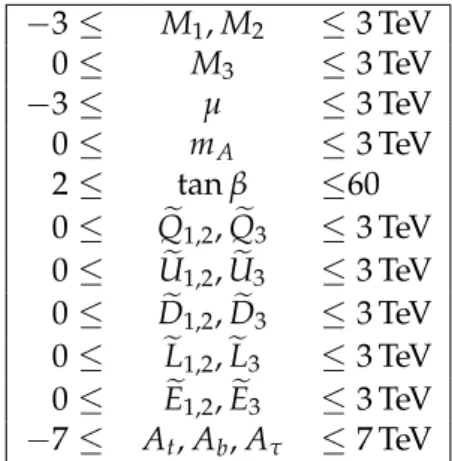
our study to the pMSSM sub-space chosen to cover sparticle masses up to about 3 TeV. Table 3 summarizes the boundaries of the considered sub-space.

Table 3: The pMSSM parameter space used in the scan.

−3≤ M1, M2 ≤3 TeV 0≤ M3 ≤3 TeV −3≤ µ ≤3 TeV 0≤ mA ≤3 TeV 2≤ tan β ≤60 0≤ Qe_1,2, eQ₃ ≤3 TeV 0≤ Ue_1,2, eU₃ ≤3 TeV 0≤ De_1,2, eD₃ ≤3 TeV 0≤ eL_1,2, eL₃ ≤3 TeV 0≤ Ee_1,2, eE₃ ≤3 TeV −7≤ At, Ab, Aτ ≤7 TeV

In Ref. [21], some previous CMS published results were reinterpreted in the context of this pMSSM sub-space. This analysis, however, did not consider the region of parameter space in which long-lived charginos are predicted. Using the technique described in Section 3, we can extend the results of Ref. [21] to regions of the parameter space leading to long-lived particles. We sample 20 million points in a pMSSM parameter space from a prior probability density function that encodes results from indirect SUSY searches and pre-LHC searches as done in Ref. [21]. From this set we select 7205 points with a Higgs boson mass in the range 120 ≤

mh ≤ 130 GeV and predicting long-lived (cτ > 50 cm) charginos. Tightening further the mass

window to 123 ≤ mh ≤128 GeV to reflect more recent constraints from the Higgs boson mass

measurements [22–24] reduces the size of the subset by 45% but does not further constrain the chargino mass or lifetime. We therefore use the 120 ≤ m_h ≤ 130 GeV window in order to minimize the statistical uncertainty.

For each of the 7205 points in this subset, we have generated 10 000 events using PYTHIA

v6.426 [25]. Both direct pair production of charginos and indirect chargino production through the decay of heavier SUSY particles were considered for this study. The generated events have

been used to evaluate the signal acceptance of the HSCP search, given the chargino kinematic properties predicted byPYTHIAfor the considered pMSSM sub-space.

The fast technique is used to obtain acceptance values expected to be in good agreement with the full simulation prediction. The predicted signal acceptance is then used to compute 95% CL limits on the 7205 analysed pMSSM parameter points. A parameter point is excluded if the ob-served limit obtained on the cross section is less than the theoretical prediction at leading-order as calculated byPYTHIA. The use of leading-order instead of next-to-leading-order theoretical cross section is driven by practical considerations given the large number of parameter points considered.

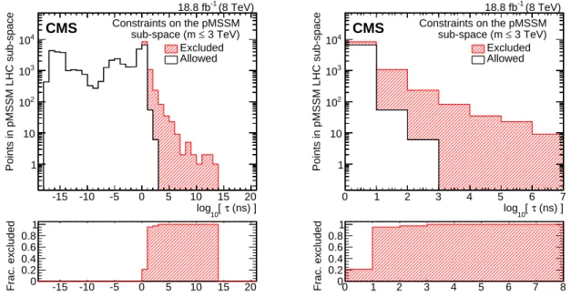
Figure 3 shows the fraction of parameter points excluded as a function of the chargino life-time. The fraction of excluded model points with a chargino lifetime longer than 1000 ns (10 ns) is 100.0% (95.9%). Although these values depend on the random point sampling in the 19-dimensional pMSSM parameter space, it is remarkable that a high fraction of the points predicting long-lived charginos are excluded.

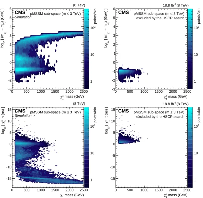
Figure 4 shows the number of parameter points predicted and excluded by the analysis of the results obtained in Ref. [12] as a function of the chargino mass, chargino lifetime, and the mass difference between the chargino and the neutralino.

(ns) ] τ [ 10 log -15 -10 -5 0 5 10 15 20 Points in pMSSM LHC sub-space 1 10 2 10 3 10 4 10 Constraints on the pMSSM 3 TeV) ≤ sub-space (m Excluded Allowed -15 -10 -5 0 5 10 15 20 Frac. excluded 0 0.2 0.4 0.6 0.8 1 (8 TeV) -1 18.8 fb CMS (ns) ] τ [ 10 log 0 1 2 3 4 5 6 7 Points in pMSSM LHC sub-space 1 10 2 10 3 10 4 10 Constraints on the pMSSM 3 TeV) ≤ sub-space (m Excluded Allowed 0 1 2 3 4 5 6 7 8 Frac. excluded 0 0.2 0.4 0.6 0.8 1 (8 TeV) -1 18.8 fb CMS

Figure 3: (left) Number of pMSSM points, in the sub-space covering sparticle masses up to about 3 TeV, that are excluded at a 95% CL (hatched red) or allowed (white) as a function of the chargino lifetime. (right) Enlargement of the long-lived region. The bottom panel shows the fraction of pMSSM points excluded by the analysis based on the results from the HSCP search [12].

5

Constraints on the AMSB model

In the AMSB model [2–4] the lightest chargino and neutralino are almost degenerate (m

e

χ±₁ − m

e

χ0₁ ≤ 1 GeV), where the neutralino is the lightest SUSY particle. In this model, the chargino lifetime, expected to be of the order of a nanosecond or larger, is determined by the mass splitting with the neutralino.

10 5 Constraints on the AMSB model mass (GeV) ± 1 χ 0 500 1000 1500 2000 2500 ) (GeV) ]0_χ1 m − ±_χ1 [ (m 10 log -3 -2 -1 0 1 2 3 4 5 6 points/bin 1 10 2 10 CMS (8 TeV)

SimulationpMSSM sub-space (m ≤ 3 TeV)

mass (GeV) ± 1 χ 0 500 1000 1500 2000 2500 ) (GeV) ]0_χ1 m − ±_χ1 [ (m 10 log -3 -2 -1 0 1 2 3 4 5 6 points/bin 1 10 2 10 (8 TeV) -1 18.8 fb CMS _{pMSSM sub-space (m ≤ 3 TeV)}

excluded by the HSCP search

mass (GeV) ± 1 χ 0 500 1000 1500 2000 2500 (ns) ] τ ±_χ 1 [ 10 log -15 -10 -5 0 5 10 15 points/bin 1 10 2 10 CMS (8 TeV)

SimulationpMSSM sub-space (m ≤ 3 TeV)

mass (GeV) ± 1 χ 0 500 1000 1500 2000 2500 (ns) ] τ ±_χ 1 [ 10 log -15 -10 -5 0 5 10 15 points/bin 1 10 2 10 (8 TeV) -1 18.8 fb CMS _{pMSSM sub-space (m ≤ 3 TeV)}

excluded by the HSCP search

Figure 4: Number of pMSSM parameter points in the sub-space covering sparticle masses up to about 3 TeV shown as a function of the chargino mass and (upper row) of the mass difference between the chargino and the neutralino, and (lower row) chargino lifetime. The left panels show the entire set of points considered while the right panels show the set of points excluded by the analysis based on the results from the HSCP search [12].

Previous searches for AMSB charginos [26, 27] looked for a chargino decaying within the track-ing volume into a neutralino and a soft charged pion. The pion has a momentum of ∼ 100 MeV and is generally not reconstructed. The experimental chargino signature therefore takes the form of a disappearing track inside the tracking system. The main limitation of that search technique is that the sensitivity drops quickly as the lifetime increases because the chargino is required to decay within the tracking region.

In contrast, the sensitivity of the search for HSCP [12] is maximal when the chargino decay occurs outside the detector. These two searches are therefore complementary. In this context, the fast technique discussed in the previous sections can be used to assess the limits set by Ref. [12] on long-lived charginos in the AMSB model.

The minimal version of the AMSB model is fully characterized by four parameters: the ratio of Higgs doublet vacuum expectation values at the electroweak scale, the sign of the higgsino mass term, the universal scalar mass (m0), and the gravitino mass (m3/2), which dictates the

value of the chargino mass. The values of the first two parameters are set to tan β = 5 and µ > 0. The scalar mass is set to a large value (1 TeV) in order to prevent the appearance of tachyonic sleptons. Gravitino masses ranging from 3.5 to 32 TeV are used in order to scan chargino masses from 100 to 900 GeV.

Samples of simulated charginos with masses from 100 to 900 GeV and lifetimes from 1 ns to 10 µs are produced with PYTHIA v6.426. The SUSY mass spectrum and the decay tables are calculated usingISASUSYwithISAJETv7.80 [28]. For each sample, 10 000 events are generated using an inclusive SUSY production and the acceptance of the search for long-lived particles is estimated using the technique described in Section 3. The estimated signal acceptance is shown in Fig. 5 (left). The acceptance is reduced for short lifetimes because the probability that a particle reaches the muon system before decaying, is exponentially smaller. As explained in Section 3, a systematic uncertainty of 25% is assigned to the signal acceptance. A point in the mass–lifetime parameter space of the AMSB model is considered to be excluded when the 95% CL observed limit on the cross section is lower than the leading-order theoretical cross section. The excluded region in this plane is shown in Fig. 5 (right). These results extend those from previous searches at LHC experiments [26, 27] by excluding charginos with lifetimes&100 ns up to masses of about 800 GeV. While the signal acceptance remains nearly constant over a wide mass range, heavier charginos cannot be excluded because of their smaller production cross section. The sensitivity of the search for HSCP [12] is limited to charginos with an average lifetime≥3 ns while previous searches based on short track signatures are sensitive to lifetimes of∼0.1 ns [26, 27].

6

Summary

The results of the CMS search for long-lived charged particles have been analysed to set con-straints on the phenomenological minimal supersymmetric standard model (pMSSM) and on the anomaly-mediated SUSY breaking model (AMSB), both of which predict the existence of long-lived massive particles in certain regions of their parameter space. A novel technique for estimating the signal acceptance with an accuracy of 10% is presented. This technique only uses generator-level information, while the integrated luminosity, the expected standard model background yields, and the corresponding uncertainties are taken from a previous CMS search [12]. The technique and the tabulated probabilities, available as supplementary material to this paper [13], can be used by others to estimate the CMS exclusion limits for different mod-els predicting long-lived lepton-like particles. In the context of the AMSB model, charginos with lifetimes& 100 ns (3 ns) and masses up to about 800 GeV (100 GeV) are excluded at 95%

12 6 Summary AMSB > 0) µ ) = 5, β (tan( Acceptance -7 10 -6 10 -5 10 -4 10 -3 10 -2 10 -1 10 mass (GeV) ± 1 χ 100 200 300 400 500 600 700 800 900 (ns) τ ±_χ 1 1 10 2 10 (8 TeV) Simulation CMS AMSB > 0) µ ) = 5, β (tan( mass (GeV) ± 1 χ 100 200 300 400 500 600 700 800 900 (ns) τ ±_χ 1 1 10 2 10 (8 TeV) -1 18.8 fb CMS AMSB > 0) µ ) = 5, β (tan( Observed limit Expected limit σ 1 ± Expected limit σ 2 ± Expected limit Excluded area

Figure 5: (left) Signal acceptance as a function of chargino mass for the AMSB model as pre-dicted by the fast technique. (right) Observed and expected excluded region on the chargino mass and lifetime parameter space in the context of the AMSB model with tan β=5 and µ≥0. The excluded region is indicated by the hatched area.

confidence level. The most stringent limits to date are set on the long-lived sector of the pMSSM sub-space that covers SUSY particle masses up to about 3 TeV. In this sub-space, 95.9% (100%) of the points with a chargino lifetime τ ≥10 ns (1000 ns) are excluded by the present analysis of the results from the CMS search in Ref. [12]. These are the first constraints on the pMSSM obtained at the LHC.

Acknowledgments

We congratulate our colleagues in the CERN accelerator departments for the excellent perfor-mance of the LHC and thank the technical and administrative staffs at CERN and at other CMS institutes for their contributions to the success of the CMS effort. In addition, we gratefully acknowledge the computing centres and personnel of the Worldwide LHC Computing Grid for delivering so effectively the computing infrastructure essential to our analyses. Finally, we acknowledge the enduring support for the construction and operation of the LHC and the CMS detector provided by the following funding agencies: BMWFW and FWF (Austria); FNRS and FWO (Belgium); CNPq, CAPES, FAPERJ, and FAPESP (Brazil); MES (Bulgaria); CERN; CAS, MoST, and NSFC (China); COLCIENCIAS (Colombia); MSES and CSF (Croatia); RPF (Cyprus); MoER, ERC IUT and ERDF (Estonia); Academy of Finland, MEC, and HIP (Finland); CEA and CNRS/IN2P3 (France); BMBF, DFG, and HGF (Germany); GSRT (Greece); OTKA and NIH (Hungary); DAE and DST (India); IPM (Iran); SFI (Ireland); INFN (Italy); MSIP and NRF (Re-public of Korea); LAS (Lithuania); MOE and UM (Malaysia); CINVESTAV, CONACYT, SEP, and UASLP-FAI (Mexico); MBIE (New Zealand); PAEC (Pakistan); MSHE and NSC (Poland); FCT (Portugal); JINR (Dubna); MON, RosAtom, RAS and RFBR (Russia); MESTD (Serbia); SEIDI and CPAN (Spain); Swiss Funding Agencies (Switzerland); MST (Taipei); ThEPCenter, IPST, STAR and NSTDA (Thailand); TUBITAK and TAEK (Turkey); NASU and SFFR (Ukraine); STFC (United Kingdom); DOE and NSF (USA).

Re-search Council and EPLANET (European Union); the Leventis Foundation; the A. P. Sloan Foundation; the Alexander von Humboldt Foundation; the Belgian Federal Science Policy Of-fice; the Fonds pour la Formation `a la Recherche dans l’Industrie et dans l’Agriculture (FRIA-Belgium); the Agentschap voor Innovatie door Wetenschap en Technologie (IWT-(FRIA-Belgium); the Ministry of Education, Youth and Sports (MEYS) of the Czech Republic; the Council of Sci-ence and Industrial Research, India; the HOMING PLUS programme of Foundation for Polish Science, cofinanced from European Union, Regional Development Fund; the Compagnia di San Paolo (Torino); the Consorzio per la Fisica (Trieste); MIUR project 20108T4XTM (Italy); the Thalis and Aristeia programmes cofinanced by EU-ESF and the Greek NSRF; and the National Priorities Research Program by Qatar National Research Fund.

References

[1] MSSM Working Group Collaboration, “The Minimal Supersymmetric Standard Model: Group Summary Report”, (1998). arXiv:hep-ph/9901246.

[2] C.-H. Chen, M. Drees, and J. F. Gunion, “Nonstandard string-SUSY scenario and its phenomenological implications”, Phys. Rev. D 55 (1997) 330,

doi:10.1103/PhysRevD.55.330, arXiv:hep-ph/9607421. [Erratum: doi:10.1103/PhysRevD.60.039901].

[3] G. F. Giudice, M. A. Luty, H. Murayama, and R. Rattazzi, “Gaugino mass without singlets”, JHEP 12 (1998) 027, doi:10.1088/1126-6708/1998/12/027, arXiv:9810.442.

[4] L. Randall and R. Sundrum, “Out of this world supersymmetry breaking”, Nucl. Phys. B

557(1999) 079, doi:10.1016/S0550-3213(99)00359-4, arXiv:hep-th/9810155. [5] S. L. Glashow, “Partial-symmetries of weak interactions”, Nucl. Phys. 22 (1961) 579,

doi:10.1016/0029-5582(61)90469-2.

[6] S. Weinberg, “A Model of Leptons”, Phys. Rev. Lett. 19 (1967) 1264, doi:10.1103/PhysRevLett.19.1264.

[7] A. Salam, “Weak and electromagnetic interactions”, in Elementary particle physics: relativistic groups and analyticity, N. Svartholm, ed., p. 367. Almqvist & Wiksell, 1968. Proceedings of the eighth Nobel symposium.

[8] H. P. Nilles, “Supersymmetry, supergravity and particle physics”, Phys. Rep. 110 (1984) 1, doi:10.1016/0370-1573(84)90008-5.

[9] N. Arkani-Hamed, S. Dimopoulos, and G. Dvali, “The hierarchy problem and new dimensions at a millimeter”, Phys. Lett. B 429 (1998) 263,

doi:10.1016/S0370-2693(98)00466-3, arXiv:hep-ph/9803315.

[10] L. Randall and R. Sundrum, “Large Mass Hierarchy from a Small Extra Dimension”, Phys. Rev. Lett. 83 (1999) 3370, doi:10.1103/PhysRevLett.83.3370,

arXiv:hep-ph/9905221.

[11] CMS Collaboration, “The CMS experiment at the CERN LHC”, JINST 3 (2008) S08004, doi:10.1088/1748-0221/3/08/S08004.

14 References

[12] CMS Collaboration, “Searches for long-lived charged particles in pp collisions at√s = 7 and 8 TeV”, JHEP 07 (2013) 122, doi:10.1007/JHEP07(2013)122,

arXiv:1305.0491.

[13] CMS Collaboration, “Supplementary material from constraints on the pMSSM, AMSB model and on other models from the search for long-lived charged particles in

proton-proton collisions at√s=8 TeV”, (2014). Deposited at HepData: http://hepdata.cedar.ac.uk/view/ins1343509.

[14] T. Junk, “Confidence level computation for combining searches with small statistics”, Nucl. Instrum. Meth. A 434 (1999) 435, doi:10.1016/S0168-9002(99)00498-2, arXiv:hep-ex/9902006.

[15] A. L. Read, “Presentation of search results: the CLstechnique”, J. Phys. G 28 (2002) 2693,

doi:10.1088/0954-3899/28/10/313.

[16] ATLAS and CMS Collaborations, “Procedure for the LHC Higgs boson search combination in Summer 2011”, Technical Report CMS-NOTE-2011-005, ATL-PHYS-PUB-2011-011, CERN, Geneva, 2011.

[17] W. T. Eadie et al., “Statistical methods in experimental physics”. North Holland, Amsterdam, 1971.

[18] F. James, “Statistical methods in experimental physics”. World Scientific, Singapore, 2006. [19] M. Fairbairn et al., “Stable massive particles at colliders”, Phys. Rept. 438 (2007) 1,

doi:10.1016/j.physrep.2006.10.002, arXiv:hep-ph/0611040.

[20] CMS Collaboration, “Search for heavy long-lived charged particles in pp collisions at_√ s =7 TeV”, Phys. Lett. B 713 (2012) 408, doi:10.1016/j.physletb.2012.06.023, arXiv:1205.0272.

[21] S. Sekmen et al., “Interpreting LHC SUSY searches in the phenomenological MSSM”, JHEP 02 (2012) 075, doi:10.1007/JHEP02(2012)075, arXiv:1109.5119.

[22] CMS Collaboration, “Measurement of the properties of a Higgs boson in the four-lepton final state”, Phys. Rev. D 89 (2014) 092007, doi:10.1103/PhysRevD.89.092007, arXiv:1312.5353.

[23] CMS Collaboration, “Observation of the diphoton decay of the Higgs boson and measurement of its properties”, Eur. Phys. J. C 74 (2014) 3076,

doi:10.1140/epjc/s10052-014-3076-z, arXiv:1407.0558.

[24] ATLAS Collaboration, “Measurement of the Higgs boson mass from the H →γγand H→ ZZ∗ →4`channels with the ATLAS detector using 25 fb−1_{of pp collision data”,}

Phys. Rev. D 90 (2014) 052004, doi:10.1103/PhysRevD.90.052004, arXiv:1406.3827.

[25] T. Sj ¨ostrand, S. Mrenna, and P. Skands, “PYTHIA 6.4 physics and manual”, JHEP 05 (2006) 026, doi:10.1088/1126-6708/2006/05/026, arXiv:hep-ph/0603175. [26] ATLAS Collaboration, “Search for charginos nearly mass degenerate with the lightest

neutralino based on a disappearing-track signature in pp collisions at√s=8 TeV with the ATLAS detector”, Phys. Rev. D 88 (2013) 206,

[27] CMS Collaboration, “Search for disappearing tracks in proton-proton collisions at√s = 8 TeV”, JHEP 01 (2015) 096, doi:10.1007/JHEP01(2015)096, arXiv:1411.6006. [28] H. Baer, F. E. Paige, S. D. Protopopescu, and X. Tata, “ISAJET 7.48: A Monte Carlo Event

Generator for pp, p ¯p, and e+e−Interactions”, (2000). arXiv:hep-ph/0001086. [29] P. Langacker and G. Steigman, “Requiem for an FCHAMP (Fractionally CHArged,

Massive Particle) ?”, Phys. Rev. D 84 (2011) 065040,

doi:10.1103/PhysRevD.84.065040, arXiv:1107.3131.

A

Details of the fast technique

The probabilities Pon(k)and Poff(mthresh, k), introduced in Section 3, are computed using

sam-ples of single long-lived particles, uniformly distributed in η and β, and produced in PYTHIA

v6.426 [25]. Twenty samples, each containing one million stau particles, were produced for the following long-lived particle masses: 100, 126, 156, 200, 247, 308, 370, 432, 494, 557, 651, 745, 871, 1029, 1200, 1400, 1600, 1800, 2000, and 2500 GeV. These generated events were then pro-cessed by the full CMS simulation and reconstruction software. The full simulation includes pileup effects. The selection requirements adopted by the “tracker+TOF” analysis described in Ref. [12] were then applied to the reconstructed events in order to evaluate the probability that a particle with kinematics k can pass the selection criteria.

The probabilities Pon_{(k)and P}off_(m

thresh, k) were evaluated in 3D bins of|η|, β, and pT. For

|η|we consider the following bin boundaries: 0.0, 0.25, 0.50, 0.75, 1.00, 1.10, 1.125, 1.50, 1.75, 2.00, 2.10. The granularity is finer around the transition between the tracker barrel and the tracker endcap to better model the efficiency in this region. Since the detector is symmetric in η, the probabilities for the positive and negative η regions were averaged in order to reduce the statistical uncertainties. A constant bin width of 0.05 is considered between 0.0 and 1.0 for the binning in β. For the binning along pT the following bin boundaries are considered 5, 50,

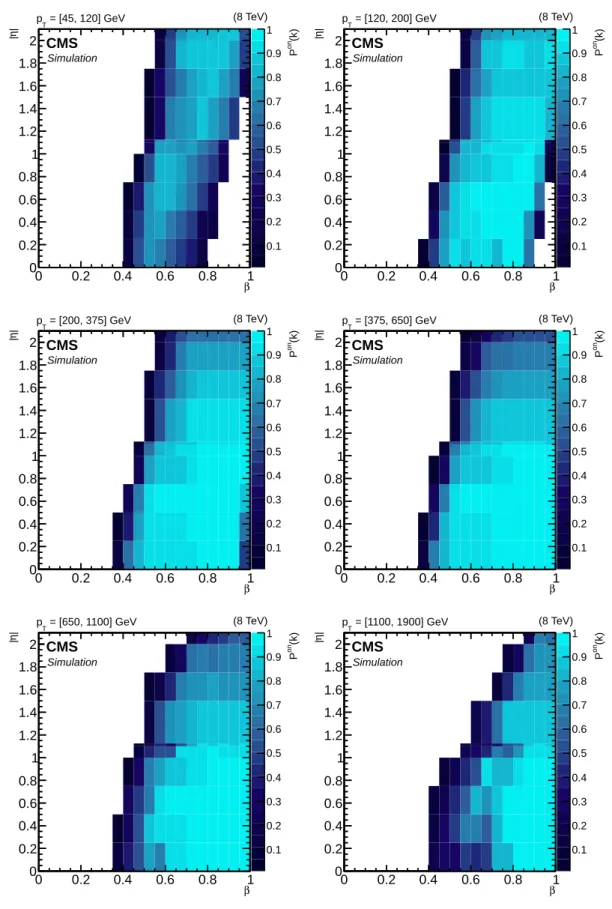
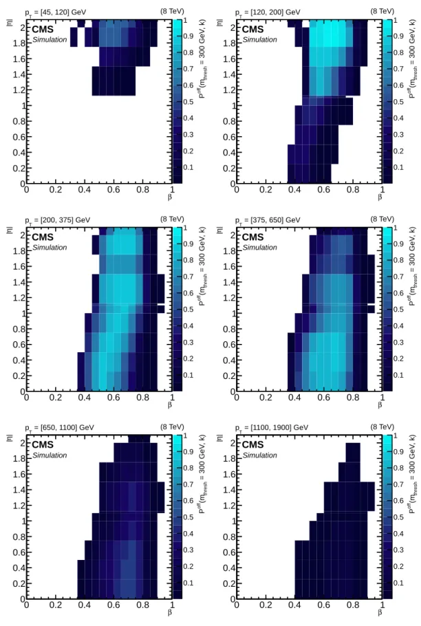
60, 70, 80, 90, 100, 110, 120, 130, 140, 150, 160, 170, 180, 190, 200, 220, 240, 260, 280, 300, 325, 350, 375, 400, 425, 450, 475, 500, 550, 600, 650, 700, 750, 800, 850, 900, 950, 1000, 1100, 1200, 1300, 1400, 1500, 1600, 1700, 1800, 1900, 2000, 2250, 2500, ∞ GeV. Figures A.1, A.2, and A.3 show the estimated values of Pon(k), Poff(0 GeV, k), and Poff(300 GeV, k), respectively. The complete evaluation of Pon(k)and Poff(mthresh, k)for the bin ranges previously described is available as

supplemental material to this paper [13].

The fast technique is validated by comparing the estimated signal acceptance values with those obtained from the full simulation for three benchmark models predicting long-lived leptons: pair production of staus, inclusive production of staus in the context of a gauge mediated sym-metry breaking (GMSB) model, and pair production of long-lived leptons with a null weak isospin [29]. These three models, having significantly different kinematic properties, are stud-ied in Ref. [12].

The signal acceptance obtained with the two methods is shown in Figs. A.4 and A.5 for the benchmark models considered for two thresholds on the reconstructed mass, mthresh. The

ac-ceptance computed with the full simulation and with the technique presented in this paper agrees within 10%. The agreement between the two techniques is worse when the mass thresh-old is close to the true mass of the long-lived particle. The larger disagreement close to the mass threshold is a consequence of the coarse binning of probability Poff(mthresh, k), which only

partially reflects the sharp variation in probability with the reconstructed values of pT, η, and

16 A Details of the fast technique

of a cutoff applied in the data acquisition electronics of the tracker detector. In Ref. [12], the threshold on the reconstructed mass is optimized for each signal model considered. In this paper, for the sake of simplicity, the threshold on the reconstructed mass used in the fast tech-nique is set at 60% of the true particle mass. The hatched area in Figs. A.4 and A.5 indicates the range not satisfying the requirement on the reconstructed mass threshold. Outside of this region the estimated signal acceptance is always compatible within 10% with the results from full simulation.

Several points of the pMSSM subset have also been fully simulated, as described in Ref. [12], in order to further validate the fast estimation of the acceptance in the context of pMSSM. The acceptances estimated using the full simulation prediction and the proposed technique are compared in Fig. A.6 for points leading to quasi-stable (cτ ≥100 m) charginos. An agreement at the level of 10% is observed.

β 0 0.2 0.4 0.6 0.8 1 | η | 0 0.2 0.4 0.6 0.8 1 1.2 1.4 1.6 1.8 2 _on(k) P 0.1 0.2 0.3 0.4 0.5 0.6 0.7 0.8 0.9 1 = [45, 120] GeV T p CMS (8 TeV) Simulation β 0 0.2 0.4 0.6 0.8 1 | η | 0 0.2 0.4 0.6 0.8 1 1.2 1.4 1.6 1.8 2 _on (k) P 0.1 0.2 0.3 0.4 0.5 0.6 0.7 0.8 0.9 1 = [120, 200] GeV T p CMS (8 TeV) Simulation β 0 0.2 0.4 0.6 0.8 1 | η | 0 0.2 0.4 0.6 0.8 1 1.2 1.4 1.6 1.8 2 (k) on P 0.1 0.2 0.3 0.4 0.5 0.6 0.7 0.8 0.9 1 = [200, 375] GeV T p CMS (8 TeV) Simulation β 0 0.2 0.4 0.6 0.8 1 | η | 0 0.2 0.4 0.6 0.8 1 1.2 1.4 1.6 1.8 2 (k) on P 0.1 0.2 0.3 0.4 0.5 0.6 0.7 0.8 0.9 1 = [375, 650] GeV T p CMS (8 TeV) Simulation β 0 0.2 0.4 0.6 0.8 1 | η | 0 0.2 0.4 0.6 0.8 1 1.2 1.4 1.6 1.8 2 _on(k) P 0.1 0.2 0.3 0.4 0.5 0.6 0.7 0.8 0.9 1 = [650, 1100] GeV T p CMS (8 TeV) Simulation β 0 0.2 0.4 0.6 0.8 1 | η | 0 0.2 0.4 0.6 0.8 1 1.2 1.4 1.6 1.8 2 _on (k) P 0.1 0.2 0.3 0.4 0.5 0.6 0.7 0.8 0.9 1 = [1100, 1900] GeV T p CMS (8 TeV) Simulation

Figure A.1: Values taken by the probability Pon_{(k)as a function of the true particle-variables}

18 A Details of the fast technique β 0 0.2 0.4 0.6 0.8 1 | η | 0 0.2 0.4 0.6 0.8 1 1.2 1.4 1.6 1.8 2 = 0 G e V , k ) thresh (m o ff P 0.1 0.2 0.3 0.4 0.5 0.6 0.7 0.8 0.9 1 = [45, 120] GeV T p CMS (8 TeV) Simulation β 0 0.2 0.4 0.6 0.8 1 | η | 0 0.2 0.4 0.6 0.8 1 1.2 1.4 1.6 1.8 2 = 0 G e V , k ) thresh (m o ff P 0.1 0.2 0.3 0.4 0.5 0.6 0.7 0.8 0.9 1 = [120, 200] GeV T p CMS (8 TeV) Simulation β 0 0.2 0.4 0.6 0.8 1 | η | 0 0.2 0.4 0.6 0.8 1 1.2 1.4 1.6 1.8 2 = 0 G e V , k ) thresh (m o ff P 0.1 0.2 0.3 0.4 0.5 0.6 0.7 0.8 0.9 1 = [200, 375] GeV T p CMS (8 TeV) Simulation β 0 0.2 0.4 0.6 0.8 1 | η | 0 0.2 0.4 0.6 0.8 1 1.2 1.4 1.6 1.8 2 = 0 G e V , k ) thresh (m o ff P 0.1 0.2 0.3 0.4 0.5 0.6 0.7 0.8 0.9 1 = [375, 650] GeV T p CMS (8 TeV) Simulation β 0 0.2 0.4 0.6 0.8 1 | η | 0 0.2 0.4 0.6 0.8 1 1.2 1.4 1.6 1.8 2 = 0 G e V , k ) thresh (m o ff P 0.1 0.2 0.3 0.4 0.5 0.6 0.7 0.8 0.9 1 = [650, 1100] GeV T p CMS (8 TeV) Simulation β 0 0.2 0.4 0.6 0.8 1 | η | 0 0.2 0.4 0.6 0.8 1 1.2 1.4 1.6 1.8 2 = 0 G e V , k ) thresh (m o ff P 0.1 0.2 0.3 0.4 0.5 0.6 0.7 0.8 0.9 1 = [1100, 1900] GeV T p CMS (8 TeV) Simulation

Figure A.2: Values taken by the probability Poff(0, k)as a function of the true particle-variables pT, β, and|η|. The binning in pTin these figures is coarser than the one used in the study.

β 0 0.2 0.4 0.6 0.8 1 | η | 0 0.2 0.4 0.6 0.8 1 1.2 1.4 1.6 1.8 2 = 3 0 0 G e V , k ) thresh (m o ff P 0.1 0.2 0.3 0.4 0.5 0.6 0.7 0.8 0.9 1 = [45, 120] GeV T p CMS (8 TeV) Simulation β 0 0.2 0.4 0.6 0.8 1 | η | 0 0.2 0.4 0.6 0.8 1 1.2 1.4 1.6 1.8 2 = 3 0 0 G e V , k ) thresh (m o ff P 0.1 0.2 0.3 0.4 0.5 0.6 0.7 0.8 0.9 1 = [120, 200] GeV T p CMS (8 TeV) Simulation β 0 0.2 0.4 0.6 0.8 1 | η | 0 0.2 0.4 0.6 0.8 1 1.2 1.4 1.6 1.8 2 = 3 0 0 G e V , k ) thresh (m o ff P 0.1 0.2 0.3 0.4 0.5 0.6 0.7 0.8 0.9 1 = [200, 375] GeV T p CMS (8 TeV) Simulation β 0 0.2 0.4 0.6 0.8 1 | η | 0 0.2 0.4 0.6 0.8 1 1.2 1.4 1.6 1.8 2 = 3 0 0 G e V , k ) thresh (m o ff P 0.1 0.2 0.3 0.4 0.5 0.6 0.7 0.8 0.9 1 = [375, 650] GeV T p CMS (8 TeV) Simulation β 0 0.2 0.4 0.6 0.8 1 | η | 0 0.2 0.4 0.6 0.8 1 1.2 1.4 1.6 1.8 2 = 3 0 0 G e V , k ) thresh (m o ff P 0.1 0.2 0.3 0.4 0.5 0.6 0.7 0.8 0.9 1 = [650, 1100] GeV T p CMS (8 TeV) Simulation β 0 0.2 0.4 0.6 0.8 1 | η | 0 0.2 0.4 0.6 0.8 1 1.2 1.4 1.6 1.8 2 = 3 0 0 G e V , k ) thresh (m o ff P 0.1 0.2 0.3 0.4 0.5 0.6 0.7 0.8 0.9 1 = [1100, 1900] GeV T p CMS (8 TeV) Simulation

Figure A.3: Values taken by the probability Poff(300 GeV, k)as a function of the true particle-variables pT, β, and|η|. The binning in pT in these figures is coarser than the one used in the

20 A Details of the fast technique

Figure A.4: Signal acceptance for a mass threshold of 0 (left) and 300 GeV (right). The upper and lower sets of distributions show the pair production and inclusive production of staus as predicted by the GMSB model, respectively. The panel below each figure shows the ratio of acceptance from the fast technique to the acceptance obtained from a full simulation of the de-tector. The hatched area indicates the range not satisfying the requirement on the reconstructed mass threshold.

Figure A.5: Signal acceptance for a mass threshold of 0 (left) and 300 GeV (right). The tested model is the pair production of leptons with no weak isospin. The panel below each figure shows the ratio of acceptance from the fast technique to the acceptance obtained from a full simulation of the detector. The hatched area indicates the range not satisfying the requirement on the reconstructed mass threshold.

Figure A.6: Signal acceptance for a mass threshold of 0 (left) and 300 GeV (right) on a few representative pMSSM points predicting quasi-stable (cτ ≥100 m) charginos. The panel below each figure shows the ratio of acceptance from the fast technique to the acceptance obtained from a full simulation of the detector. The hatched area indicates the range not satisfying the requirement on the reconstructed mass threshold.

B

The CMS Collaboration

Yerevan Physics Institute, Yerevan, Armenia

V. Khachatryan, A.M. Sirunyan, A. Tumasyan

Institut f ¨ur Hochenergiephysik der OeAW, Wien, Austria

W. Adam, T. Bergauer, M. Dragicevic, J. Er ¨o, M. Friedl, R. Fr ¨uhwirth1, V.M. Ghete, C. Hartl, N. H ¨ormann, J. Hrubec, M. Jeitler1, W. Kiesenhofer, V. Kn ¨unz, M. Krammer1, I. Kr¨atschmer, D. Liko, I. Mikulec, D. Rabady2_{, B. Rahbaran, H. Rohringer, R. Sch ¨ofbeck, J. Strauss,}

W. Treberer-Treberspurg, W. Waltenberger, C.-E. Wulz1

National Centre for Particle and High Energy Physics, Minsk, Belarus

V. Mossolov, N. Shumeiko, J. Suarez Gonzalez

Universiteit Antwerpen, Antwerpen, Belgium

S. Alderweireldt, S. Bansal, T. Cornelis, E.A. De Wolf, X. Janssen, A. Knutsson, J. Lauwers, S. Luyckx, S. Ochesanu, R. Rougny, M. Van De Klundert, H. Van Haevermaet, P. Van Mechelen, N. Van Remortel, A. Van Spilbeeck

Vrije Universiteit Brussel, Brussel, Belgium

F. Blekman, S. Blyweert, J. D’Hondt, N. Daci, N. Heracleous, J. Keaveney, S. Lowette, M. Maes, A. Olbrechts, Q. Python, D. Strom, S. Tavernier, W. Van Doninck, P. Van Mulders, G.P. Van Onsem, I. Villella

Universit´e Libre de Bruxelles, Bruxelles, Belgium

C. Caillol, B. Clerbaux, G. De Lentdecker, D. Dobur, L. Favart, A.P.R. Gay, A. Grebenyuk, A. L´eonard, A. Mohammadi, L. Perni`e2, A. Randle-conde, T. Reis, T. Seva, L. Thomas, C. Vander Velde, P. Vanlaer, J. Wang, F. Zenoni

Ghent University, Ghent, Belgium

V. Adler, K. Beernaert, L. Benucci, A. Cimmino, S. Costantini, S. Crucy, A. Fagot, G. Garcia, J. Mccartin, A.A. Ocampo Rios, D. Poyraz, D. Ryckbosch, S. Salva Diblen, M. Sigamani, N. Strobbe, F. Thyssen, M. Tytgat, E. Yazgan, N. Zaganidis

Universit´e Catholique de Louvain, Louvain-la-Neuve, Belgium

S. Basegmez, C. Beluffi3, G. Bruno, R. Castello, A. Caudron, L. Ceard, G.G. Da Silveira, C. Delaere, T. du Pree, D. Favart, L. Forthomme, A. Giammanco4, J. Hollar, A. Jafari, P. Jez, M. Komm, V. Lemaitre, C. Nuttens, L. Perrini, A. Pin, K. Piotrzkowski, A. Popov5, L. Quertenmont, M. Selvaggi, M. Vidal Marono, J.M. Vizan Garcia

Universit´e de Mons, Mons, Belgium

N. Beliy, T. Caebergs, E. Daubie, G.H. Hammad

Centro Brasileiro de Pesquisas Fisicas, Rio de Janeiro, Brazil

W.L. Ald´a J ´unior, G.A. Alves, L. Brito, M. Correa Martins Junior, T. Dos Reis Martins, J. Molina, C. Mora Herrera, M.E. Pol, P. Rebello Teles

Universidade do Estado do Rio de Janeiro, Rio de Janeiro, Brazil

W. Carvalho, J. Chinellato6, A. Cust ´odio, E.M. Da Costa, D. De Jesus Damiao, C. De Oliveira Martins, S. Fonseca De Souza, H. Malbouisson, D. Matos Figueiredo, L. Mundim, H. Nogima, W.L. Prado Da Silva, J. Santaolalla, A. Santoro, A. Sznajder, E.J. Tonelli Manganote6, A. Vilela Pereira

24 B The CMS Collaboration

Universidade Estadual Paulistaa, Universidade Federal do ABCb, S˜ao Paulo, Brazil

C.A. Bernardesb, S. Dograa, T.R. Fernandez Perez Tomeia, E.M. Gregoresb, P.G. Mercadanteb, S.F. Novaesa, Sandra S. Padulaa

Institute for Nuclear Research and Nuclear Energy, Sofia, Bulgaria

A. Aleksandrov, V. Genchev2, R. Hadjiiska, P. Iaydjiev, A. Marinov, S. Piperov, M. Rodozov, S. Stoykova, G. Sultanov, M. Vutova

University of Sofia, Sofia, Bulgaria

A. Dimitrov, I. Glushkov, L. Litov, B. Pavlov, P. Petkov

Institute of High Energy Physics, Beijing, China

J.G. Bian, G.M. Chen, H.S. Chen, M. Chen, T. Cheng, R. Du, C.H. Jiang, R. Plestina7, F. Romeo, J. Tao, Z. Wang

State Key Laboratory of Nuclear Physics and Technology, Peking University, Beijing, China

C. Asawatangtrakuldee, Y. Ban, S. Liu, Y. Mao, S.J. Qian, D. Wang, Z. Xu, L. Zhang, W. Zou

Universidad de Los Andes, Bogota, Colombia

C. Avila, A. Cabrera, L.F. Chaparro Sierra, C. Florez, J.P. Gomez, B. Gomez Moreno, J.C. Sanabria

University of Split, Faculty of Electrical Engineering, Mechanical Engineering and Naval Architecture, Split, Croatia

N. Godinovic, D. Lelas, D. Polic, I. Puljak

University of Split, Faculty of Science, Split, Croatia

Z. Antunovic, M. Kovac

Institute Rudjer Boskovic, Zagreb, Croatia

V. Brigljevic, K. Kadija, J. Luetic, D. Mekterovic, L. Sudic

University of Cyprus, Nicosia, Cyprus

A. Attikis, G. Mavromanolakis, J. Mousa, C. Nicolaou, F. Ptochos, P.A. Razis, H. Rykaczewski

Charles University, Prague, Czech Republic

M. Bodlak, M. Finger, M. Finger Jr.8

Academy of Scientific Research and Technology of the Arab Republic of Egypt, Egyptian Network of High Energy Physics, Cairo, Egypt

Y. Assran9_{, S. Elgammal}10_{, A. Ellithi Kamel}11_{, A. Radi}12,10

National Institute of Chemical Physics and Biophysics, Tallinn, Estonia

M. Kadastik, M. Murumaa, M. Raidal, A. Tiko

Department of Physics, University of Helsinki, Helsinki, Finland

P. Eerola, M. Voutilainen

Helsinki Institute of Physics, Helsinki, Finland

J. H¨ark ¨onen, V. Karim¨aki, R. Kinnunen, M.J. Kortelainen, T. Lamp´en, K. Lassila-Perini, S. Lehti, T. Lind´en, P. Luukka, T. M¨aenp¨a¨a, T. Peltola, E. Tuominen, J. Tuominiemi, E. Tuovinen, L. Wendland

Lappeenranta University of Technology, Lappeenranta, Finland

DSM/IRFU, CEA/Saclay, Gif-sur-Yvette, France

M. Besancon, F. Couderc, M. Dejardin, D. Denegri, B. Fabbro, J.L. Faure, C. Favaro, F. Ferri, S. Ganjour, A. Givernaud, P. Gras, G. Hamel de Monchenault, P. Jarry, E. Locci, J. Malcles, J. Rander, A. Rosowsky, M. Titov

Laboratoire Leprince-Ringuet, Ecole Polytechnique, IN2P3-CNRS, Palaiseau, France

S. Baffioni, F. Beaudette, P. Busson, E. Chapon, C. Charlot, T. Dahms, M. Dalchenko, L. Dobrzynski, N. Filipovic, A. Florent, R. Granier de Cassagnac, L. Mastrolorenzo, P. Min´e, I.N. Naranjo, M. Nguyen, C. Ochando, G. Ortona, P. Paganini, S. Regnard, R. Salerno, J.B. Sauvan, Y. Sirois, C. Veelken, Y. Yilmaz, A. Zabi

Institut Pluridisciplinaire Hubert Curien, Universit´e de Strasbourg, Universit´e de Haute Alsace Mulhouse, CNRS/IN2P3, Strasbourg, France

J.-L. Agram13, J. Andrea, A. Aubin, D. Bloch, J.-M. Brom, E.C. Chabert, C. Collard, E. Conte13, J.-C. Fontaine13, D. Gel´e, U. Goerlach, C. Goetzmann, A.-C. Le Bihan, K. Skovpen, P. Van Hove

Centre de Calcul de l’Institut National de Physique Nucleaire et de Physique des Particules, CNRS/IN2P3, Villeurbanne, France

S. Gadrat

Universit´e de Lyon, Universit´e Claude Bernard Lyon 1, CNRS-IN2P3, Institut de Physique Nucl´eaire de Lyon, Villeurbanne, France

S. Beauceron, N. Beaupere, C. Bernet7, G. Boudoul2, E. Bouvier, S. Brochet, C.A. Carrillo Montoya, J. Chasserat, R. Chierici, D. Contardo2, B. Courbon, P. Depasse, H. El Mamouni, J. Fan, J. Fay, S. Gascon, M. Gouzevitch, B. Ille, T. Kurca, M. Lethuillier, L. Mirabito, A.L. Pequegnot, S. Perries, J.D. Ruiz Alvarez, D. Sabes, L. Sgandurra, V. Sordini, M. Vander Donckt, P. Verdier, S. Viret, H. Xiao

Institute of High Energy Physics and Informatization, Tbilisi State University, Tbilisi, Georgia

I. Bagaturia14

RWTH Aachen University, I. Physikalisches Institut, Aachen, Germany

C. Autermann, S. Beranek, M. Bontenackels, M. Edelhoff, L. Feld, A. Heister, K. Klein, M. Lipinski, A. Ostapchuk, M. Preuten, F. Raupach, J. Sammet, S. Schael, J.F. Schulte, H. Weber, B. Wittmer, V. Zhukov5

RWTH Aachen University, III. Physikalisches Institut A, Aachen, Germany

M. Ata, M. Brodski, E. Dietz-Laursonn, D. Duchardt, M. Erdmann, R. Fischer, A. G ¨uth, T. Hebbeker, C. Heidemann, K. Hoepfner, D. Klingebiel, S. Knutzen, P. Kreuzer, M. Merschmeyer, A. Meyer, P. Millet, M. Olschewski, K. Padeken, P. Papacz, H. Reithler, S.A. Schmitz, L. Sonnenschein, D. Teyssier, S. Th ¨uer

RWTH Aachen University, III. Physikalisches Institut B, Aachen, Germany

V. Cherepanov, Y. Erdogan, G. Fl ¨ugge, H. Geenen, M. Geisler, W. Haj Ahmad, F. Hoehle, B. Kargoll, T. Kress, Y. Kuessel, A. K ¨unsken, J. Lingemann2, A. Nowack, I.M. Nugent, C. Pistone, O. Pooth, A. Stahl

Deutsches Elektronen-Synchrotron, Hamburg, Germany

M. Aldaya Martin, I. Asin, N. Bartosik, J. Behr, U. Behrens, A.J. Bell, A. Bethani, K. Borras, A. Burgmeier, A. Cakir, L. Calligaris, A. Campbell, S. Choudhury, F. Costanza, C. Diez Pardos, G. Dolinska, S. Dooling, T. Dorland, G. Eckerlin, D. Eckstein, T. Eichhorn, G. Flucke, J. Garay Garcia, A. Geiser, A. Gizhko, P. Gunnellini, J. Hauk, M. Hempel15, H. Jung, A. Kalogeropoulos, O. Karacheban15, M. Kasemann, P. Katsas, J. Kieseler, C. Kleinwort, I. Korol,

26 B The CMS Collaboration

D. Kr ¨ucker, W. Lange, J. Leonard, K. Lipka, A. Lobanov, W. Lohmann15, B. Lutz, R. Mankel, I. Marfin15, I.-A. Melzer-Pellmann, A.B. Meyer, G. Mittag, J. Mnich, A. Mussgiller, S. Naumann-Emme, A. Nayak, E. Ntomari, H. Perrey, D. Pitzl, R. Placakyte, A. Raspereza, P.M. Ribeiro Cipriano, B. Roland, E. Ron, M. ¨O. Sahin, J. Salfeld-Nebgen, P. Saxena, T. Schoerner-Sadenius, M. Schr ¨oder, C. Seitz, S. Spannagel, A.D.R. Vargas Trevino, R. Walsh, C. Wissing

University of Hamburg, Hamburg, Germany

V. Blobel, M. Centis Vignali, A.R. Draeger, J. Erfle, E. Garutti, K. Goebel, M. G ¨orner, J. Haller, M. Hoffmann, R.S. H ¨oing, A. Junkes, H. Kirschenmann, R. Klanner, R. Kogler, T. Lapsien, T. Lenz, I. Marchesini, D. Marconi, J. Ott, T. Peiffer, A. Perieanu, N. Pietsch, J. Poehlsen, T. Poehlsen, D. Rathjens, C. Sander, H. Schettler, P. Schleper, E. Schlieckau, A. Schmidt, M. Seidel, V. Sola, H. Stadie, G. Steinbr ¨uck, D. Troendle, E. Usai, L. Vanelderen, A. Vanhoefer

Institut f ¨ur Experimentelle Kernphysik, Karlsruhe, Germany

C. Barth, C. Baus, J. Berger, C. B ¨oser, E. Butz, T. Chwalek, W. De Boer, A. Descroix, A. Dierlamm, M. Feindt, F. Frensch, M. Giffels, A. Gilbert, F. Hartmann2, T. Hauth, U. Husemann, I. Katkov5, A. Kornmayer2, P. Lobelle Pardo, M.U. Mozer, T. M ¨uller, Th. M ¨uller, A. N ¨urnberg, G. Quast, K. Rabbertz, S. R ¨ocker, H.J. Simonis, F.M. Stober, R. Ulrich, J. Wagner-Kuhr, S. Wayand, T. Weiler, R. Wolf

Institute of Nuclear and Particle Physics (INPP), NCSR Demokritos, Aghia Paraskevi, Greece

G. Anagnostou, G. Daskalakis, T. Geralis, V.A. Giakoumopoulou, A. Kyriakis, D. Loukas, A. Markou, C. Markou, A. Psallidas, I. Topsis-Giotis

University of Athens, Athens, Greece

A. Agapitos, S. Kesisoglou, A. Panagiotou, N. Saoulidou, E. Stiliaris, E. Tziaferi

University of Io´annina, Io´annina, Greece

X. Aslanoglou, I. Evangelou, G. Flouris, C. Foudas, P. Kokkas, N. Manthos, I. Papadopoulos, E. Paradas, J. Strologas

Wigner Research Centre for Physics, Budapest, Hungary

G. Bencze, C. Hajdu, P. Hidas, D. Horvath16, F. Sikler, V. Veszpremi, G. Vesztergombi17, A.J. Zsigmond

Institute of Nuclear Research ATOMKI, Debrecen, Hungary

N. Beni, S. Czellar, J. Karancsi18, J. Molnar, J. Palinkas, Z. Szillasi

University of Debrecen, Debrecen, Hungary

A. Makovec, P. Raics, Z.L. Trocsanyi, B. Ujvari

National Institute of Science Education and Research, Bhubaneswar, India

S.K. Swain

Panjab University, Chandigarh, India

S.B. Beri, V. Bhatnagar, R. Gupta, U.Bhawandeep, A.K. Kalsi, M. Kaur, R. Kumar, M. Mittal, N. Nishu, J.B. Singh

University of Delhi, Delhi, India

Ashok Kumar, Arun Kumar, S. Ahuja, A. Bhardwaj, B.C. Choudhary, A. Kumar, S. Malhotra, M. Naimuddin, K. Ranjan, V. Sharma

Saha Institute of Nuclear Physics, Kolkata, India

S. Banerjee, S. Bhattacharya, K. Chatterjee, S. Dutta, B. Gomber, Sa. Jain, Sh. Jain, R. Khurana, A. Modak, S. Mukherjee, D. Roy, S. Sarkar, M. Sharan

Bhabha Atomic Research Centre, Mumbai, India

A. Abdulsalam, D. Dutta, V. Kumar, A.K. Mohanty2, L.M. Pant, P. Shukla, A. Topkar

Tata Institute of Fundamental Research, Mumbai, India

T. Aziz, S. Banerjee, S. Bhowmik19, R.M. Chatterjee, R.K. Dewanjee, S. Dugad, S. Ganguly, S. Ghosh, M. Guchait, A. Gurtu20, G. Kole, S. Kumar, M. Maity19, G. Majumder, K. Mazumdar, G.B. Mohanty, B. Parida, K. Sudhakar, N. Wickramage21

Indian Institute of Science Education and Research (IISER), Pune, India

S. Sharma

Institute for Research in Fundamental Sciences (IPM), Tehran, Iran

H. Bakhshiansohi, H. Behnamian, S.M. Etesami22, A. Fahim23, R. Goldouzian, M. Khakzad, M. Mohammadi Najafabadi, M. Naseri, S. Paktinat Mehdiabadi, F. Rezaei Hosseinabadi, B. Safarzadeh24_{, M. Zeinali}

University College Dublin, Dublin, Ireland

M. Felcini, M. Grunewald

INFN Sezione di Baria, Universit`a di Barib, Politecnico di Baric, Bari, Italy

M. Abbresciaa,b, C. Calabriaa,b, S.S. Chhibraa,b, A. Colaleoa, D. Creanzaa,c, L. Cristellaa,b, N. De Filippisa,c, M. De Palmaa,b, L. Fiorea, G. Iasellia,c, G. Maggia,c, M. Maggia, S. Mya,c, S. Nuzzoa,b, A. Pompilia,b_{, G. Pugliese}a,c_{, R. Radogna}a,b,2_{, G. Selvaggi}a,b_{, A. Sharma}a_{, L. Silvestris}a,2_,

R. Vendittia,b, P. Verwilligena

INFN Sezione di Bolognaa, Universit`a di Bolognab, Bologna, Italy

G. Abbiendia, A.C. Benvenutia, D. Bonacorsia,b, S. Braibant-Giacomellia,b, L. Brigliadoria,b, R. Campaninia,b, P. Capiluppia,b, A. Castroa,b, F.R. Cavalloa, G. Codispotia,b, M. Cuffiania,b, G.M. Dallavallea, F. Fabbria, A. Fanfania,b, D. Fasanellaa,b, P. Giacomellia, C. Grandia, L. Guiduccia,b, S. Marcellinia, G. Masettia, A. Montanaria, F.L. Navarriaa,b, A. Perrottaa, A.M. Rossia,b_{, T. Rovelli}a,b_{, G.P. Siroli}a,b_{, N. Tosi}a,b_{, R. Travaglini}a,b

INFN Sezione di Cataniaa, Universit`a di Cataniab, CSFNSMc, Catania, Italy

S. Albergoa,b, G. Cappelloa, M. Chiorbolia,b, S. Costaa,b, F. Giordanoa,c,2, R. Potenzaa,b, A. Tricomia,b, C. Tuvea,b

INFN Sezione di Firenzea, Universit`a di Firenzeb, Firenze, Italy

G. Barbaglia, V. Ciullia,b, C. Civininia, R. D’Alessandroa,b, E. Focardia,b, E. Galloa, S. Gonzia,b, V. Goria,b_{, P. Lenzi}a,b_{, M. Meschini}a_{, S. Paoletti}a_{, G. Sguazzoni}a_{, A. Tropiano}a,b

INFN Laboratori Nazionali di Frascati, Frascati, Italy

L. Benussi, S. Bianco, F. Fabbri, D. Piccolo

INFN Sezione di Genovaa, Universit`a di Genovab, Genova, Italy

R. Ferrettia,b, F. Ferroa, M. Lo Veterea,b, E. Robuttia, S. Tosia,b

INFN Sezione di Milano-Bicoccaa, Universit`a di Milano-Bicoccab, Milano, Italy

M.E. Dinardoa,b, S. Fiorendia,b, S. Gennaia,2, R. Gerosaa,b,2, A. Ghezzia,b, P. Govonia,b, M.T. Lucchinia,b,2, S. Malvezzia, R.A. Manzonia,b, A. Martellia,b, B. Marzocchia,b,2, D. Menascea, L. Moronia, M. Paganonia,b, D. Pedrinia, S. Ragazzia,b, N. Redaellia, T. Tabarelli de Fatisa,b