2016
UNIVERSIDADE DE LISBOA
FACULDADE DE CIÊNCIAS
DEPARTAMENTO DE BIOLOGIA ANIMAL
The relative importance of clade age, ecology and life-history
traits in mammalian species richness
Pedro Miguel Santos Neves
Mestrado em Biologia Evolutiva e do Desenvolvimento
Dissertação orientada por:
Prof. Carlos Fernandes
Prof. Fernando Ascensão
ii
Acknowledgments
I want to thank my advisors for taking me as their student and for all their help and encouragement during this year. I thank Prof. Carlos Fernandes for introducing me to this particular “brand” of Evolution and Ecology, for his help and knowledge in the design of the project, during the analyses, discussion, and in revising the manuscript. I also thank Dr. Fernando Ascensão for his assistance and support during the entire project, and for patiently teaching me how to conduct statistical analyses in R and showing me the importance of communicating clearly and concisely.
I am very grateful for the collaboration and friendship of Dr. Luís Borda de Água, who always had a helping hand, and also introduced me to a number of interesting topics and concepts in Ecology, Evolution, and Statistics through several enjoyable conversations and discussions.
I would also like to express my gratitude to Dr. Manuela González-Suárez for her participation in the project, her very helpful suggestions of databases, and for taking the time to patiently and kindly teach me how to fit and interpret mixed models, as well as how to properly display results and much more. I thank everyone from the THEOECO and APPLECOL groups from CIBIO at ISA for having me for a short talk and all their helpful comments, as well as for putting up with me during lunch and lab meetings whenever I ran to Fernando and Luís for help. In particular, I acknowledge the very helpful brainstorming sessions with Dr. César Capinha and Dr. Rafael Barrientos about the inclusion of ecological data in the final dataset.
I thank all my friends, for helping me stay sane, and for forgiving my absence whenever I was working late at night.
I thank Carolina Barata for all the help she gave me before, and ever since this Dissertation started. For sharing this passion for Evolution and Biology with me. And for sharing my successes and failures, for hearing me despair when things went wrong but never letting me lose hope. For always being there to help, even when the distance was great.
Finally, I thank my parents and my grandma, whose help and support have been constant since long before I started this dissertation. I’m grateful for their patience, kindness during the more hectic days, for believing in me, for reading my work and for their thoughts, and for always being there. I’m sure everything would have been a lot more difficult without them.
iii
Abstract
Extant mammalian clades have very different degrees of species richness, as some groups contain a very large number of species while others are represented by only one. The causes for this asymmetry remain undetermined. We gathered data for 14 variables classified in three groups: biogeography, ecology, and life-history. We also included clade age as an additional variable, to test the hypothesis that older clades, having had more time to diversify, contain more species. By using several online databases, we were able to include 4514 mammal species belonging to 1096 genera, 127 families, and 27 orders, making this, to our knowledge, the most comprehensive study on the drivers of mammalian species richness. Our analysis, which consisted in a generalized linear model, was conducted at three taxonomic levels: genus, family, and order. This allowed us to verify if the effect of a given variable is consistent regardless of the taxonomic hierarchical level. Our results suggest that clade age is not related to species richness regardless of the taxonomic level of analysis. We found that biogeography, namely, geographic range size and latitude were the most important variables, but with different effects. We found geographic range size to have a negative relationship with mammalian species richness, while latitude has a positive relationship. The intragroup variability of adult body mass was also important in some cases, although this might be due to the correlation of body mass with other variables. Generation length appears more important than litter size, but its weak signal makes drawing conclusions difficult. Ecological variables were the least important ones, with the sole exception of trophic level diversity at the genus level. However, it is possible that the ecological variables used did not capture well the most important ecological factors influencing clade species richness. Overall, our study points the major role of biogeography at influencing diversification rate in mammals.
Keywords: species richness, clade age, life-history, ecology, biogeography
Resumo
Existe uma grande disparidade na riqueza específica entre os vários grupos animais. A maioria das espécies encontra-se distribuída por um número reduzido de ordens, famílias e géneros, tendo a maior parte dos grupos taxonómicos poucas espécies extantes. A idade dos clados (ou grupos monofiléticos) é uma explicação clássica deste fenómeno, através da hipótese de que clados mais antigos terão tido mais tempo para sofrer processos de especiação e, por conseguinte, que o número de espécies nesses clados seja maior. Contudo, esta hipótese ignora ou minimiza o papel da extinção, que reduz o número de espécies, e que terá tido mais oportunidades de ocorrência em clados mais antigos. O número de espécies extantes resulta, portanto do balanço entre especiação e extinção, normalmente designada por taxa de diversificação, que naturalmente pode não ser constante no tempo. Vários trabalhos têm procurado explicar a assimetria e heterogeneidade na riqueza específica entre diferentes clados recorrendo a diversas abordagens, mas frequentemente estudando a relação entre riqueza específica e um pequeno número de variáveis. Não existe ainda um consenso claro sobre as variáveis mais importantes na determinação da riqueza específica dos clados, pois são conhecidos exemplos contraditórios para várias hipóteses, sendo o mais provável que uma multiplicidade de factores esteja envolvida em simultâneo.
iv Neste estudo investigámos o efeito e a importância relativa de variáveis que podem afectar a taxa de diversificação e, consequentemente, o número de espécies de mamíferos em grupos taxonómicos supraespecíficos. A classe dos mamíferos é ideal para um estudo desta natureza porque a sua história evolutiva é bastante bem conhecida, existe bastante informação para espécies de mamíferos, e o número de espécies é elevado o suficiente para permitir inferir padrões globais, mas sem ser tão numeroso que torne excessivamente complexo e difícil o manuseamento dos dados.
Ao contrário da maioria da literatura sobre o assunto, procurámos realizar uma análise abrangente e assim incluímos três grupos de variáveis que podem influenciar a riqueza específica de mamíferos. Obtivemos os dados a partir de várias bases de dados disponíveis online, para um total final em análise de 4154 espécies de mamíferos (pertencentes a 1096 géneros, 127 famílias e 27 ordens) filtradas de um total de 5156 espécies existentes disponíveis na base de dados de referência, PanTHERIA. Para além da idade de cada clado, incluímos:
Variáveis biogeográficas: tamanho da área de distribuição e a sua variação, latitude e longitude; Características biológicas e da história de vida: número de indivíduos por ninhada, tempo de
geração, e massa corporal dos adultos, assim como o coeficiente de variação de cada um; Variáveis ecológicas: diversidade de níveis tróficos, diversidade de dieta, diversidade de
actividade, e diversidade de estratégias de forrageamento, representadas pelo índice de Shannon de cada categoria em cada nível taxonómico.
Recorremos então a um modelo linear generalizado. Utilizando uma abordagem de inferência multimodelo obtivemos as variáveis mais importantes de cada grupo, a incluir num modelo final com variáveis de todos os grupos. Por fim, calculámos da mesma forma a importância relativa de cada um dos factores incluídos no modelo final.
Para verificar se o efeito de cada um destes grupos de variáveis é consistente independentemente do nível taxonómico a que é feita a análise, o processo foi realizado ao nível do género, família e ordem, utilizando sempre que necessário a média de uma dada variável por grupo taxonómico, ou o índice de diversidade de Shannon no caso das variáveis ecológicas.
As variáveis biogeográficas constituem o grupo de variáveis mais importante que identificámos a qualquer um dos níveis taxonómicos. A latitude, o tamanho da área de distribuição e o seu coeficiente de variação apresentam valores altos de importância. Ao nível da ordem, apesar de apenas a latitude surgir no topo da importância, o seu índice é mais baixo e nenhuma variável é identificada como estatisticamente significativa. Isto sugere que o seu efeito será real a qualquer um dos níveis, mas que o aumento da variância associado ao nível da ordem pode tornar o sinal mais difícil de obter. O tamanho da área de distribuição está negativamente relacionado com a diversidade, o que indica que terá um efeito negativo na taxa de especiação ou positivo na taxa de extinção, apesar desta segunda hipótese nos parecer menos provável. Por sua vez, verificámos que a variabilidade do tamanho da área de distribuição está positivamente associada à diversidade. Propomos que estas observações se devam ao facto de que espécies com menores áreas de distribuição poderão permitir a persistência de um maior número de espécies numa dada área geográfica, e a uma elevada importância da especiação alopátrica. O facto de grandes áreas de distribuição poderem conferir maior resistência à extinção, pode não compensar o seu potencial impacto negativo na especiação.
As características da história de vida estudadas aparentam ter uma influência muito pequena na riqueza específica. A variação da massa corporal aparenta ter um efeito, especialmente aos níveis da família e ordem. No entanto, a massa corporal está correlacionada com várias outras características intrínsecas
v das espécies que podem afectar a especiação e a extinção. Um resultado interessante, por ser contrário a resultados descritos em trabalhos anteriores em mamíferos, é o tempo de geração aparentemente contribuir mais para a diversidade de mamíferos do que o número de crias por ninhada. Estas características são altamente variáveis entre grupos taxonómicos e as diferentes importâncias relativas entre estudos podem ser devidas a diferenças nos taxa estudados. Será talvez devido a estas diferenças que obtivemos resultados diferentes relativamente a outros estudos. Contudo, tendo em conta a muito maior escala a que este trabalho foi efectuado, concluímos que, a nível global, o tempo de geração é a variável estudada da história de vida que mais impacto tem na diversidade de mamíferos.
Dos três grupos de variáveis, o das variáveis ecológicas foi o menos importante. A única variável ecológica a apresentar alguma importância foi a diversidade do nível trófico ao nível do género. Noutros trabalhos, foi encontrada uma relação entre o nível trófico e a especiação em mamíferos, tendo-se verificado que as espécies herbívoras têm em geral uma maior taxa de especiação, e as omnívoras uma menor taxa de especiação. Sugerimos que a importância da diversidade trófica que verificámos no estudo possa ser o resultado de duas causas. Por um lado, a diversidade de nível trófico contribui para a redução de extinções causadas por grandes alterações abióticas e bióticas que afectem a disponibilidade de recursos em diferentes níveis tróficos. Por outro lado, a diversidade de nível trófico tenderá a diminuir a competição entre espécies do mesmo género, o que por sua vez deverá ter um impacto negativo nas taxas de extinção e positivo nas taxas de especiação.
Os nossos resultados confirmam, tal como anteriormente concluído por vários autores, que a idade dos clados não é um factor explicativo da sua riqueza específica. A taxa de diversificação não será, portanto, constante no tempo para os diversos clados de mamíferos.
Neste estudo desenvolvemos uma abordagem o mais abrangente e exaustiva possível para tentar identificar variáveis importantes na determinação da riqueza especifica de taxa a diferentes níveis hierárquicos dentro de grandes grupos taxonómicos. Identificámos uma elevada importância de variáveis biogeográficas, que se sobrepõe a todas as outras variáveis em qualquer dos níveis taxonómicos que analisámos, na riqueza específica em mamíferos. O nosso trabalho sugere que, apesar da importância de certos factores variar entre clados, a importância da biogeografia é dominante globalmente.
vi
Contents
Acknowledgments ...ii Abstract ... iii Resumo ... iii Contents ... vi 1. Introduction ... 12. Materials and methods ... 3
2.1 Data acquisition ... 3
2.2 Model fitting and selection ... 7
3. Results ... 9
1. Discussion ... 19
References ... 23
Supporting Information ... 26
Figure index
Figure 2.1. Flowchart of the GLM data analysis. ... 8Figure 3.1. Histogram of species richness (n = 4514) across 127 mammalian families. ... 10
Figure 3.2. Histogram of species richness (n = 4514) across 27 mammalian orders. ... 10
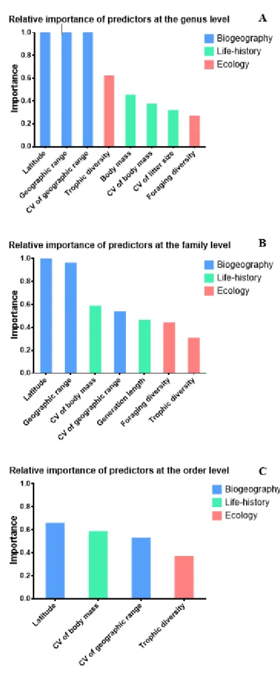
Figure 3.3. Relative importance plots for the variables in the final global models. The vertical bars represent the relative importance of the variables in the analyses at the genus (A), family (B), and order (C) levels. ... 14
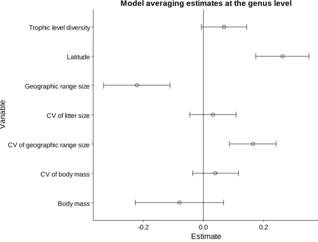
Figure 3.4. Estimates obtained by averaging the best models (ΔAICc ≤ 2) at the genus level. Horizontal bars represent 95% confidence intervals. ... 16
Figure 3.5. Estimates obtained by averaging the best models (ΔAICc ≤ 2) at the family level. Horizontal bars represent 95% confidence intervals. ... 17
Figure 3.6. Estimates obtained by averaging the best models (ΔAICc ≤ 2) at the order level. Horizontal bars represent 95% confidence intervals. ... 18
Table index
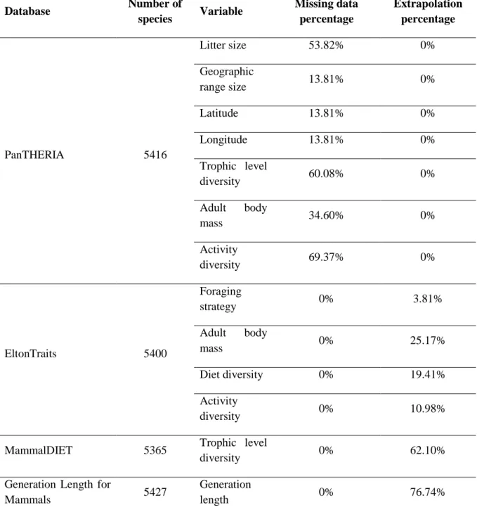
Table 2.1.1. Groups of predictors and variables. Data sources databases are coded as follows: P – PanTHERIA; M – MammalDIET, E – EltonTraits; G - Generation Length for Mammals ... 5Table 2.1.2. Data source databases with number of species, and missing data and extrapolation percentages in the variables used. ... 6
Table 2.2.1. Importance values obtained in the separate analyses for each variable group at the different taxonomic levels. ... 12
Table 2.2.2. Importance values obtained in the final global models for the different taxonomic levels. ... 13
1
1. Introduction
The causes of species richness in each clade of life have long been sought after by evolutionary biologists. The species richness of a clade results from the balance of the effects of speciation and extinction rates. The difference between speciation and extinction rates is usually called diversification rate (Stadler 2011). A constantly positive diversification rate results in a net increase in extant richness, as extinction does not offset speciation. On the other hand, a negative diversification rate implies that extinction prevails over speciation resulting in a net decrease in species richness.
The diversification rate is different across clades. In fact, one of the most prevalent and obvious patterns in the tree of life is the unevenness in the number of species among higher taxa. For example, in mammals, some families are comprised of several hundred species, an extreme example being the Muridae with 730 species, but most families are not particularly diverse, with many having a single species. This is the case of the Orycteropodidae whose only extant member is the aardvark (Orycteropus afer). Intuitively, species richness could positively correlate with clade age, as older clades have had more time to undergo speciation events and thus diversify (McPeek and Brown 2007). However, this relationship is far from linear, and several examples directly contradict it, with old clades having few species. This may be due to an inherent decline in speciation rates with time or an increase in extinction rates, which will ultimately result in the extinction of a clade. Conversely, in younger clades, speciation and extinction rates may reach equilibrium after an initial burst of speciation, which will transiently maintain the net number of species constant through time.
What, then, explains such diverse patterns of species richness? The debate on the exact dynamics of diversification rates is far from settled, with theoretical and empirical studies supporting both the importance of clade age (McPeek and Brown 2007; Bloom et al. 2014) or its decoupling from species richness and its causes (Ricklefs 2007; Rabosky 2009; Rabosky et al. 2012; Verde Arregoitia et al. 2013). The latter studies suggest that there may be several variables at play shaping species richness. Several variables have been proposed, most of which we can classify into three groups: ecological, biological life-history traits, and biogeographical.
Given the contrasting conclusions of the aforementioned studies, in this investigation we aimed to determine the relative importance of clade age and of some variables of those variable groups, as well as the relative importance of individual variables, in mammalian species richness.
Ecological traits are specific traits related to resource acquisition and coping with the environment.
Resource acquisition is extremely important for the success of individuals and populations, and it can therefore play a part in a species’ vulnerability to extinction and probability to persist and speciate. For example, species at higher trophic levels are generally considered more sensitive to environmental change, and hence more likely to become extinct (Purvis et al. 2000). On the other hand, trophic specialization is known to correlate with diversification rate, with higher specialization leading to greater diversification (Price et al. 2012). Additionally, analyses of diet diversity may provide finer-grained insights into the importance of trophic ecology and its influence on speciation and extinction rates.
Biological and life-history traits are variables related to intrinsic characteristics of species. Many of
such variables have a potential effect on the abundance, and consequently on the effective population size, of a clade, and thus on diversification rates. Indeed, researchers have found life-history traits to
2 have such an impact (Isaac et al. 2005). A short generation length and a high number of offspring per litter and smaller body size are correlated with abundance (Marzluff and Dial 1991; White et al. 2007). Abundance is the number of individuals in a population, or, in this case, in a species (Smith and Smith 2011). High abundance should provide more opportunities for speciation. From a genetic perspective, species with larger effective population sizes are expected to be more genetically diverse (Frankham 1996), and a greater amount of standing genetic variation can facilitate ecological speciation (Schluter and Conte 2009). Body size is negatively linked to abundance and is known to have a complex relationship with the prediction of extinction (Cardillo et al. 2005). In contrast, life-history traits, such as litter size and age of sexual maturity, have been found to be good predictors of extinction risk (González-Suárez and Revilla 2013).
Biogeographic characteristics of a species’ distribution, such as range size, have long been identified
as having an effect in species richness across the globe (Ricklefs et al. 2007; Rabosky 2009). For instance, species richness varies along a latitudinal gradient, with the tropics possessing the highest diversity (Brown and Lomolino 1998; Pyron and Wiens 2013). Moreover, species with a larger distribution are likely to occupy a greater number of different habitats. Such species may be more resistant to environmental change and as such, more likely to persist. However, if we consider allopatric speciation to be the main, or one of the most important, modes of speciation, it can be argued that broad and continuous distributions of ecologically flexible species lowers speciation rates and cladogenesis. Nevertheless, Cardillo and colleagues (2003) tested such hypotheses using Australian mammals and found a positive correlation between range size and diversification rates. Other studies identified small range sizes as being correlated with increased extinction risks (Purvis et al. 2000; Manne and Pimm 2001). Biogeographical variables are also linked with resource availability in a number of ways, an example being higher net primary productivity near the tropics (Gillman et al. 2015).
In this study, we investigated several variables belonging to the three types of variables described above, to identify the most relevant ones in shaping species richness across higher taxonomic levels in mammals. We aimed to determine if any group of factors is particularly crucial in explaining species richness patterns, and for that purpose we used both taxonomically informed and non-informed generalized linear models. We further assessed whether results were consistent across taxonomic ranks by repeating the analyses at the genus, family, and order levels.
We focused on the Mammalia class for three different reasons. First, its evolutionary history is generally well understood (Beck et al. 2006). Second, it contains a large enough number of species to allow reliable results without being unwieldy. Finally, restricting the analysis to a single high-taxonomic level clade makes variables more comparable between species. Our study included 4514 mammalian species and 14 variables from three groups of predictors. To our knowledge, this is the first research assessing simultaneously the relative importance of traits related to species’ ecology, biology and life history, and biogeography, as well as clade age, in determining species richness in mammals.
3
2. Materials and methods
2.1 Data acquisition
We assembled a dataset of variables pertaining to the three major groups of potential predictors discussed above. Some of the variables result from calculations on the raw data. See Table 2.1.1 for a full list of variables, their short description, and data source databases.
We scaled and standardized all continuous variables and log transformed the response variable: number of species per taxonomic group (González-Suárez and Revilla 2013).
We retrieved species data on litter size, adult body mass in grams, geographic range size in km2,
maximum and minimum latitude and longitude in degrees from the PanTHERIA database (Jones et al. 2009). PanTHERIA is the most widely used database for mammals, comprising information for 5416 species, and it was the primary data source for this work. We also gathered activity, foraging strategy, trophic level, body mass, and diet information from the EltonTraits database (Wilman et al. 2014). EltonTraits has high data coverage and relatively little data extrapolation (81% of diet data, 89% of activity data, and 96% foraging information are considered certain). Whenever possible, we completed body mass data missing in PanTHERIA with information from EltonTraits. We further obtained data on generation length from the database Generation Length for Mammals (Pacifici et al. 2013), and on trophic level from the MammalDIET database (Kissling et al. 2014), with the latter also used to complete missing values in the PanTHERIA dataset. Some of these databases use imputation or extrapolation to complete missing values, and the percentage of such cases is given in Table 2.1.2. We computed missing data percentages for all species and removed from the study those with 20% or more missing values. Then, we checked if any family had a missing data percentage greater than 10%; whenever this was the case, the taxon was removed from the dataset. A list of removed taxa is given in Table S 2.-Table S 3. It would have been interesting to include other variables, such as age of sexual maturity, weaning age, abundance/density, and number of litters per year, but missing data for these variables was too high. Clade ages were obtained from the TimeTree database (Hedges et al. 2015). TimeTree consists of a compilation of dating studies, with clade age estimates usually calculated by several methods and using different data (molecular and/or fossil), and the final value for each taxon corresponds to the mean of all studies. Occasionally, TimeTree estimates are the mean from a small number of studies with wildly different results. Given this, we took the following approach: if the difference between the mean and median of all studies for a given taxon was over 10% of the mean, we used the age estimate from either a single study or the mean of two studies, whenever two were available. Molecular studies on a single taxon were preferred over class wide studies and supertrees and over fossil dating (see Supporting Information Table S 1 for information on the literature used). We did not include clade age information in the analysis at the genus level due to the high number of genera (1230 in PanTHERIA) and the impossibility of obtaining quality data for all.
For taxonomy, we followed Wilson and Reeder’s (2005) Mammal Species of the World and the IUCN Red List of Threatened Species (IUCN 2016). We compared and checked the taxonomy of the used databases and corrected inconsistencies.
We ended with three datasets for analysis arranged by taxonomic level, with species grouped by genus, family, and order, respectively. With the exception of latitude and longitude, we summarized continuous variables for each clade by calculating mean values across species. For each taxonomic level, we examined whether the mean was an appropriate descriptor of central tendency for all variables by
4 visually inspecting the cumulative mean (using randomly sorted values in three randomized plots per variable) to confirm that the values generally converged to a constant value. We then compared these results with those using the same procedure but with the median. Means were judged as a better representation of the data than medians, and therefore used in the analyses (see Supporting Information Figure S 1). For latitude and longitude, we calculated the difference between the maximum and minimum values within each clade. We hypothesized that the mode of the body mass could provide insight into the diversification potential of a clade since, for a similar geographic range, significantly distinct values of body mass may entail substantially different speciation and extinction rates. We divided the range of adult body mass of each clade into four modal classes of equal size, and the mean of the most frequent modal class was calculated and included in the analyses.
To obtain a single value per clade for activity, diet, foraging strategy, and trophic level, we used the Shannon-Wiener diversity index. This method has been applied to compare diets among species (Vezzosi et al. 2014). We also included in the analyses the coefficient of variation (CV =σ
μ) of each
clade for adult body mass, generation length, litter size, and geographic range size, to test the importance of variability in these variables.
5
Table 2.1.1. Groups of predictors and variables. Data sources databases are coded as follows: P – PanTHERIA; M – MammalDIET, E – EltonTraits; G - Generation Length for Mammals
Variable group Code Variable Calculated statistic Sources
Ecology
Act Activity diversity Shannon diversity index P, E Diet Diet diversity Shannon diversity index E
TrL Trophic level
diversity Shannon diversity index P, M FrgS Foraging strategy Shannon diversity index E
Biology and life-history
BdM Adult body mass Average P, E BdM_CV Adult body mass
CV Coefficient of variation P, E BdM_M Adult body mass
mode Average P, E GnL Generation length Average G GnL_CV Generation length coefficient of variation Coefficient of variation G
LS Litter size Average P
LS_CV Litter size CV Coefficient of variation P
Biogeography
GRS Geographic
range size Average P
GRS_CV Geographic
range size CV Average P
Lat Latitude
Difference between highest and lowest latitude values in degrees of a given taxonomic group P Lon Longitude Difference between highest and lowest longitude values in degrees of a given taxonomic group
6
Table 2.1.2. Data source databases with number of species, and missing data and extrapolation percentages in the variables used. Database Number of species Variable Missing data percentage Extrapolation percentage PanTHERIA 5416 Litter size 53.82% 0% Geographic range size 13.81% 0% Latitude 13.81% 0% Longitude 13.81% 0% Trophic level diversity 60.08% 0% Adult body mass 34.60% 0% Activity diversity 69.37% 0% EltonTraits 5400 Foraging strategy 0% 3.81% Adult body mass 0% 25.17% Diet diversity 0% 19.41% Activity diversity 0% 10.98%
MammalDIET 5365 Trophic level
diversity 0% 62.10%
Generation Length for
Mammals 5427
Generation
7
2.2 Model fitting and selection
We modelled the number of species per clade as a function of the different predictors considered using negative binomial Generalized Mixed Effects Models (GLMMs). Taxa sharing an evolutionary history are not independent (Felsenstein 1985). For this reason, the model was informed taxonomically by including as a random effect the taxonomic level above that being used in the analysis. In the analysis at the taxonomic level of Order, the Superorder was used as a random effect. Afterwards, the resulting models were compared with those obtained using simpler negative binomial Generalized Linear Models (GLMs), not taking into account the relationships of taxa at each taxonomic level. As justified below, the GLM models were used in the final analysis and interpretation.
Multicollinearity among predictors was evaluated by calculating the variance inflation factors (VIF) separately for each group of variables using the function “vif” from the package “car” (Fox and Weisberg 2011). VIF is a measure of the impact of collinearity in the observed regression coefficients. Zuur et al. (2010) state that values as high as 10 have been used as a threshold for assessing multicollinearity, but recommended a more conservative value of three. We calculated pairwise Pearson correlations between selected predictors to check for the presence of highly correlated variables; whenever such cases were found, we removed one variable from each pair. Overdispersion was checked by calculating the ratio between the residual deviance and the residual degrees of freedom. A ratio < 2 was considered acceptable. Authors generally consider a dispersion parameter between 0,5 and 2 to be acceptable (Logan 2010).
After fitting all variable groups, we performed automated model selection followed by model averaging using all models. The relative importance of each variable within each variable group was calculated using the functions “dredge”, “model.avg” and “importance” from the package MuMIn (Barton 2016). Any variable with an importance value greater than 0.60 within its respective group was included in the final global model. This approach enabled us to select only the most important variables for the final models in order to keep these as parsimonious as possible. The automatic model selection output was used to calculate averages of the estimates from all models with ΔAICc ≤ 2. The 95% confidence intervals of the estimates were computed by bootstrapping the data 1000 times using the function “confint”. This whole procedure (Fig. 1) was carried out at each of the three taxonomic levels considered. All analyses were done in R (R Core Team (R Foundation for Statistical Computing) 2015) using the function “glmer.nb” from the package lme4 (Bates et al. 2015) and the function “glm.nb” from the package MASS (Venables and Ripley 2002) to fit the GLMM and GLM, respectively.
8
Figure 2.1. Flowchart of the GLM data analysis.
Obtain data for each
group + clade age
GLM within each
variable group
Model selection to
calculate
importance
Store variables with
importance > 0.60
Full GLM with all
stored variables
from all groups
Model selection to
determine
importance
Model averaging to
obtain estimates and
95% confidence
intervals
9
3. Results
After removing 902 species with high levels of missing data, the final dataset consisted of a total of 4514 species from 1096 genera, 127 families, and 27 orders. This corresponds to a coverage of 83% of all mammal species included in PanTHERIA. Most species that were removed were marine mammals, for which ecological data are largely unavailable (see Table S 2 and Table S 3 for a list of the excluded taxa). Fifteen (12%) of the families included had either no clade age estimate available in TimeTree or the difference between mean and median was over 10%. In these cases, ages were manually obtained from publications, so that in the end we did not have clade age information for only three of the 127 families (see Table S 1 for the list of families and respective clade age references).
Species were asymmetrically distributed among supraspecific taxa. Approximately 25% of the families had more than 30 species, but most families (≈ 66%) had less than 20 species. A similar pattern was also observed at the order level (Figure 3.1 and Figure 3.2).
Latitude and longitude were highly correlated (r > 0.8) at all taxonomic levels considered, and therefore longitude was discarded from the final analysis to prevent collinearity issues. Other variables also showed correlation, namely body mass and generation length (r ≈ 0.7). This may be partly due to the extrapolation used in the ‘Generation Length for Mammals’ database, the level of which is very high in several taxonomic groups. Nevertheless, because of the potential importance of both variables, we decided to include both in the analysis. Body mass mode was discarded as it was highly correlated with mean body mass (r ≈ 0.99).
Some evidence of multicollinearity was found for the life-history variables at the Order level. Nonetheless, VIF values were always < 5 and Pearson’s correlations were not extreme (e.g. body mass vs. generation length: r = 0.76), and so we chose to include both in the analyses. We found no overdispersion at any taxonomic level, as the ratio between residual deviance and degrees of freedom were low or close to one. Some models, however, showed a certain degree of underdispersion. We opted to include underdispersed models because the risk is to increase the type II error rate but not the type I error rate.
10
Figure 3.1. Histogram of species richness (n = 4514) across 127 mammalian families.
Figure 3.2. Histogram of species richness (n = 4514) across 27 mammalian orders.
0 20 40 60 0 200 400 600 Number of species N u m b e r o f fa m il ie s
Distribution of species richness across families
0 5 10 0 500 1000 1500 Number of species N u m b e r o f o rd e rs
11 All GLMMs yielded zero or close to zero random effect variance. On the other hand, GLMs exhibited identical estimates and standard errors to those from GLMMs. This indicates that, for all taxonomic levels considered, informing the models with taxonomy does not result in an increase in explanatory power. Hence, we decided to conduct the analyses without mixed models.
We constructed models separately for each variable group to select the most important variables (importance > 0.60) in each group. The estimated importance values and selected variables (importance values in bold) are given in Table 2.2.1. We then used the most important variables selected in the group-level analyses to fit the final global model for each taxonomic group-level. The variables and estimated importance values from these analyses are shown in Table 2.2.2.
Among the biogeographical variables analysed, latitude and the coefficient of variation of geographic range were selected for the final models at all taxonomic levels. Geographic range was selected at the genus and family levels (importance ≈ 1 in both cases), but not at the order level, despite its reasonable correlation with latitude. Among the biological and life-history traits, the coefficient of variation of body mass was the only one selected at all taxonomic levels, while generation length and the coefficient of variation of litter size were only selected at the Genus and Family level, respectively. Trophic level diversity was the most selected ecological trait, and the only among these that was selected at all taxonomic levels. Foraging strategy was selected at the Genus and Family level, while diet and activity were only selected at the Order and Genus level, respectively. The importance value of clade age was always low, never exceeding 0.40, and therefore it was not included in any of the final models.
We found that the group of biogeographical variables generally included those with the highest relative importance (Table 2.2.2 and Figure 3.3). This was particularly evident in the analyses at the genus and family levels, where the importance values for biogeographical variables are almost always equal or very close to one. At the Order level, the importance values were low overall, with latitude having the highest value at 0.65, followed by litter size CV with 0.58 (Table 2.2.2 and Figure 3.3 C). Variables in the ‘biological and life-history traits’ group generally ranked between those of the ‘biogeographical’ and ‘ecological’ groups. Variables in the former group ranged from very low importance (0.31: litter size CV at the Genus level) to relatively important (0.58: body mass CV at the Family level). The ecological variables generally ranked lowest in the final models, with the exception of trophic level diversity, which, with an importance value of 0.62, ranked higher than any biological and life-history trait at the Genus level (Table 2.2.2 and Figure 3.3 A). This pattern was not observed at the family and order levels, where ecological variables always ranked lowest with values never exceeding 0.45.
12
Table 2.2.1. Importance values obtained in the separate analyses for each variable group at the different taxonomic levels.
Variable
group Variable Genus Family Order
Ecology
Activity diversity 0.289 0.445 0.197
Diet diversity 0.268 0.428 0.511
Trophic level diversity 1.000 0.990 0.741
Foraging strategy 0.972 0.890 0.246
Clade age – 0.271 0.189
Biology and life–history
Adult body mass 0.630 0.358 0.278 Adult body mass CV 0.771 0.909 0.861
Generation length 0.280 0.713 0.220 Generation length CV 0.444 0.274 0.266 Litter size 0.310 0.287 0.209 Litter size CV 0.859 0.315 0.218 Clade age – 0.391 0.167 Biogeography
Geographic range size 1.000 0.969 0.349 Geographic range size
CV 1.000 0.671 0.648
Latitude 1.000 1.000 0.991
13
Table 2.2.2. Importance values obtained in the final global models for the different taxonomic levels.
Variable
group Variable Genus Family Order
Ecology
Trophic level diversity 0.618 0.302 0.366
Foraging strategy 0.263 0.436 –
Biology and life–history
Adult body mass 0.448 – –
Adult body mass CV 0.369 0.582 0.582
Generation length – 0.460 –
Litter size CV 0.313 – –
Biogeography
Geographic range size 0.999 0.958 – Geographic range size
CV 0.999 0.532 0.525
14
Figure 3.3. Relative importance plots for the variables in the final global models. The vertical bars represent the relative importance of the variables in the analyses at the genus (A), family (B), and order (C) levels.
15 Finally, we calculated the averages and 95% confidence intervals of the best models obtained with the automatic model selection procedure. The model averaging plots show the degree and direction of the effect of the most important variables on species richness (Figure 3.4-Figure 3.6). Variables that were important at more than one taxonomic level had a consistent effect direction between levels.
Latitude was found to have a positive effect on species richness at the three taxonomic levels studied, while geographic range size was found to have a negative effect at both the genus and family levels. Moreover, the average estimate values suggest a positive effect of the CV of geographic range size at all taxonomic levels, but except for the genus level the lower boundaries of the confidence intervals overlapped zero. Similarly, the results indicated a positive effect of the CV of body mass at all taxonomic levels, but only for orders did the confidence intervals not overlap zero. The average estimates also pointed to a positive effect of trophic level diversity across taxonomic levels, but the lower boundaries of the confidence intervals always overlapped zero. All other variables were selected in only one taxonomic level (genus: body mass and CV of litter size; family: generation length and foraging strategy diversity) and in all cases the confidence intervals overlapped zero.
16
Figure 3.4. Estimates obtained by averaging the best models (ΔAICc ≤ 2) at the genus level. Horizontal bars represent 95% confidence intervals.
Body mass CV of body mass CV of geographic range size CV of litter size Geographic range size Latitude Trophic level diversity
-0.2 0.0 0.2 Estimate V a ri a b le
17
Figure 3.5. Estimates obtained by averaging the best models (ΔAICc ≤ 2) at the family level. Horizontal bars represent 95% confidence intervals.
CV of body mass CV of geographic range size Foraging strategy diversity Generation length Geographic range size Latitude Trophic level diversity
-0.25 0.00 0.25 Estimate V a ri a b le
18
Figure 3.6. Estimates obtained by averaging the best models (ΔAICc ≤ 2) at the order level. Horizontal bars represent 95% confidence intervals.
CV of body mass CV of geographic range size Latitude Trophic level diversity
0.0 0.2 0.4 0.6 Estimate V a ri a b le
19
1. Discussion
The aim of this study was to investigate possible causes for differences in species richness between mammalian groups, both in general and at different supraspecific taxonomic levels.
Clade age might seem one of the most intuitive factors shaping species richness. Older clades have had more time for speciation and this could lead to a net increase in the number of species over time. While this hypothesis has been supported in previous research (McPeek and Brown 2007), it has also been contradicted by some studies (Ricklefs 2007; Rabosky 2009; Rabosky et al. 2012; Verde Arregoitia et al. 2013). Our results agree with the latter reports in suggesting that clade age is decoupled from species richness. Although, unfortunately, we could not include clade age in the Genus-level analysis, due to the lack of reliable estimates for many genera, clade age was not important enough to be included in the final models at the Family and Order levels.
Several other variables had a much greater influence on species richness than clade age. Variables in the biogeographical group, namely latitude and geographic range and its CV, generally showed high relative importance values from Genus to Order. The consistent high ranking of biogeographical variables regardless of taxonomic level indicates a high influence of biogeography on species richness. The high significance of latitude is unsurprising, given the long know latitudinal gradient of species richness (Brown and Lomolino 1998; Pyron and Wiens 2013). We found a higher latitude range to correlate with species richness. A higher latitude range may result in a higher probability of occupying the more species rich tropical region. The negative effect of geographic range size at the Family and Genus levels suggests that range size, instead of contributing to a positive diversification rate, may slow speciation rates to an extent not compensated for by its potential protective effect against extinction (Jablonski and Roy 2003, but see Gaston 1998 for a discussion on the hypotheses regarding relationship between speciation, extinction, and range size). At the evolutionary scale, allopatric speciation may be more important for species richness than resilience to extinction provided by ecological generalism. Moreover, the positive effect of the CV of geographic range size, albeit the 95% confidence interval did not overlap with zero only at the Genus level, may indicate that range size diversity is also a driver of species richness. However, this may not necessarily be the case since the positive association between the CV of geographic range size and species richness could simply reflect the fact that taxa with more species are likely to have a greater diversity of species’ geographic range sizes. In addition, it is possible that groups currently having high CV in geographic range size include species that were mostly widely distributed historically but which distributions have variably shrunk due to human impact (Boivin et al. 2016), thereby leading to an overestimation of the historical range size diversity in many groups. Nevertheless, the CV of geographic range size may have an effect. The Genus-level dataset has more data points, each derived from a smaller number of species and as such one would expect genera to have inherently lower CV values. However, we could detect an important and significant effect of the CV of geographic range size on the species richness of genera, whereas in the Order- and Family-level analyses the significance of the effect of the CV of geographic range size was unclear. This may suggest that the signal of the effect of the CV of geographic range size is not a statistical artefact resulting from the influence of taxa with high species richness. The observed positive association between the CV of geographic range size and species richness may indirectly reflect the effect of other factors, such as biological and ecological traits, but is not necessarily a by-product of high species richness. Geographic ranges appear to be highly heritable (Hunt et al. 2005; Waldron 2007), including in mammals (Jones et al. 2005). This implies that, typically, related species may tend to have similar ranges and hence variation in range size within taxa
20 should be due to other processes (for example, historical, ecological, etc.) and not simply a function of the species richness of taxa.
Due to the lack of data for many species, we unfortunately could not include dispersal ability as a variable in our study. High dispersal capacity may allow the exploration of a wide range of different habitats, and this could promote speciation, but low dispersal ability should lead to increased rates of allopatric speciation. The CV of geographic range size might be expected to be inversely correlated with dispersal capabilities. The negative effect of geographic range size together with the positive effect of the CV of geographic range size can be interpreted as indicating that susceptibility to vicariance, ecological or habitat specialism, and limited dispersal are the most influential factors increasing the net diversification rate (Bohonak 1999; Claramunt et al. 2012; Salisbury et al. 2012).
The biological and life history traits we studied appear to play a much smaller role than the biogeographical variables in shaping species richness. This is an interesting result since the previous most comprehensive analysis of the correlates of species richness in mammals (Isaac et al. 2005) mostly focused on biological and life history traits. That study, conducted at the Order level and examining four orders (Carnivora, Chiroptera, Marsupialia, and Primates), found species richness to be significantly correlated with litter size, gestation period and interbirth interval, while in our investigation neither litter size nor generation length were relatively important or statistically significant variables affecting species richness. Like ours, their study found no evidence that mammalian species richness is associated with adult body mass, but importantly we obtained some support for a positive effect of the CV of body mass, a variable they did not consider that is correlated with traits that may influence species richness (Cardillo et al. 2005, 2008). Conversely, Isaac et al. (2005) found some support for a correlation between species richness and abundance, a variable that we would have liked to have included in our analysis but for which data is lacking for many species. The different findings of the two studies are unsurprising given the differences in the number and nature of the variables considered, number and taxonomic level of the taxa analysed, sample sizes, and statistical approaches for data analysis (GLM vs. phylogenetically independent contrasts). For example, Isaac et al. (2005) did not use summary statistics of species data to characterize and represent supraspecific taxa as we did, but instead conducted their analyses at the species level. On the other hand, they analysed relatively narrow sets of taxa and variables and did not evaluate the importance and effects of variables at different taxonomic levels. Nevertheless, both studies support the idea that a host of factors influence species richness and that the major determinants may vary between taxonomic groups. For instance, Isaac et al. (2005) found that species richness is correlated with shorter gestation period in the carnivores and larger litter size in marsupials, while abundance correlates positively with species richness in primates and negatively in microchiropterans. Our Order-level analysis, where fewer variables were selected for the final model and their relative importance never exceeded 0.65, suggests that analyses at higher taxonomic levels may be confounded by high variability within taxa and may have difficulties in identifying important influencing factors.
The results for the ecological variables were remarkable in the sense that their importance was generally low. It is important to note, however, that a range of potentially important ecological variables could not be included due to a lack of data. Moreover, the ecological variables were coded in such a way that only the effect of the variable’s variation, and not the presence of a particular variable’s value, could be assessed. The only relatively important ecological variable was trophic level diversity, for which the final models indicated a positive effect on species richness at all taxonomic levels, albeit with weak statistical support. The importance of trophic level diversity may stem from two different causes. Firstly, trophic level diversity should help to reduce competition for resources between related species, especially those congeneric because, as mentioned above, they may tend to inhabit the same
21 geographical regions (Hunt et al. 2005; Waldron 2007). Secondly, trophic level diversity may provide greater resilience to environmental and habitat changes, and thereby decrease extinction rates.
It should be noted that current geographic ranges can vary wildly from the ones found throughout most of a given species’ evolutionary history, particularly given the impact of anthropogenic factors starting at the first human migrations up to the industrial revolution (Boivin et al. 2016). In fact, it has been found that accounting for the differences between historical and current ranges sizes yields different results when predicting extinction risk (Hanna and Cardillo 2013). This may be due to the different factors driving extinction currently, as opposed to the time before humans had a such a drastic impact on the environment, which could mean that current geographic ranges are a consequence and not a cause of extinction (Hanna and Cardillo 2013). Incorporating historical ranges will be required in future work. However, to dismiss that current biogeographical patterns are, at least in part, linked to a species’ evolutionary history is impossible, as it must have been influenced by dispersal and by climatic events. The problem persists in how to acquire and incorporate historical biogeographical data. The uncertainty of such inferences can introduce unwanted variance which may end up hindering our understanding of speciation and extinction patterns. However, ignoring historical biogeography potentially misrepresents the effect of these variables on speciation and extinction rates.
The concept of species also raises important challenges on diversity and speciation/extinction studies that must be recognized. Most works on species richness use the number of species per taxonomic group, geographic location, or a similar grouping factor. However, the number of species can vary wildly according to which species concept is used (Hey 2001) and as more species are discovered and described. In 19 years (1982-2001), the number of described primate species grew by more than twofold (Isaac and Purvis 2004). To circumvent this issue we used standard databases which follow a popular reference taxonomy (Wilson and Reeder 2005). This provides a good degree of comparability with other publications on this topic. However, while comparisons between studies are possible, the true number of extant species is ever changing (as more species are discovered and taxonomy is refined), and depends on the particular species concept used.
On the same topic, count creep, that is, the revision of a previously described species into two or more new species, is another concern. Count creep does not occur randomly, being more frequent among emblematic species or the ones more easily available to systematists (Isaac and Purvis 2004), which can lead to a skewed perception of richness. Isaac and Purvis (2004) verified that there is no impact in regression slopes of several ecological and life history traits with primate taxonomy changes, but did find an effect on the significance values of their results. This means that the possibility of incorrectly interpreting the dependent variable is possible, especially by diluting the effect of factors which contribute only slightly to richness.
Finally, one should bear in mind that the analyses at the Order level are inherently more artificial. We expected a much weaker signal at this level, since each taxon is comprised of a higher number species, and possesses more within group diversity. However, a sufficiently strong effect of a particular variable may still be identified. The inclusion of data surmised at the Genus level attempts to further assess impact of intragroup variability, as well as confirm the general trends found in model fitting. We confirm that this method is applicable to identify variables with a very strong effect, as we encountered for biogeography.
The ambitious scope of the work, which included more than 80% of the species present in the PanTHERIA database and incorporated a wealth of different variables allows us confidently point to biogeography as the most important factors in predicting mammal species richness. Our approach
22 adequately identifies variables that are relevant across all levels of analysis. Similarly, it hints to other possibly more elusive variables, such as generation length. Further studies should focus on disentangling and measuring the effect of the weaker variables across mammal orders, to better quantify and understand why they are important only in some cases. Whenever possible, phylogenetic information should be included for dependence correction.
It must be noted that we used several databases to ensure that our data were as complete as possible, which raises some concern. On the one hand, a higher amount of data should lead to more accurate results, since we are able to sample from a much broader range of mammals when compared with previous studies on the subject. On the other hand, several of the databases we used to complement PanTHERIA use imputation, that is, several species’ entries do not result from direct observation retrieved from the literature, but instead are extrapolations from related species. Since missing data in such databases does not occur at random, the validity of conclusions drawn from imputed values has been questioned (González-Suárez et al. 2012). Researchers have shown that predicting extinction risk from imputation heavy data leads to biased results. Due to time constraints, we assumed imputed data were as valid as direct observation, however, future work should focus on removing imputed data, resulting in a smaller, but more reliable dataset. In addition, the effect of missing data should be explored, to ensure that by removing imputed data we are not introducing bias but in a different way. We could asses this by randomly removing variables from the final dataset to gauge the effect of missing values.
23
References
Barton, K. 2016. MuMIn: Multi-Model Inference.
Bates, D., M. Mächler, B. Bolker, and S. Walker. 2015. Fitting Linear Mixed-Effects Models
Using lme4. Journal of Statistical Software 67:1–48.
Beck, R. M., O. R. Bininda-Emonds, M. Cardillo, F.-G. Liu, and A. Purvis. 2006. A
higher-level MRP supertree of placantal mammals. BMC Evolutionary Biology 6:93.
Bloom, D. D., M. Fikáček, and A. E. Z. Short. 2014. Clade age and diversification rate
variation explain disparity in species richness among water scavenger beetle (Hydrophilidae)
lineages. PLoS ONE 9.
Bohonak, A. J. 1999. Dispersal, Gene Flow, and Population Structure. The Quarterly Review
of Biology 74:21–45.
Boivin, N. L., M. A. Zeder, D. Q. Fuller, A. Crowther, G. Larson, J. M. Erlandson, T.
Denham, et al. 2016. Ecological consequences of human niche construction: Examining
long-term anthropogenic shaping of global species distributions. Proceedings of the National
Academy of Sciences 113:6388–6396.
Brown, J. H., and M. V. Lomolino. 1998. Species Diversity in Continental and Marine
Habitats. Pages 450–461 inBiogeography (2nd ed.). Sinauer Associates, Inc., Sunderland
(MA).
Cardillo, M., J. S. Huxtable, and L. Bromham. 2003. Geographic range size, life history and
rates of diversification in Australian mammals. Journal of Evolutionary Biology 16:282–288.
Cardillo, M., G. M. Mace, J. L. Gittleman, K. E. Jones, J. Bielby, and A. Purvis. 2008. The
predictability of extinction: biological and external correlates of decline in mammals.
Proceedings of the Royal Society B: Biological Sciences 275:1441–1448.
Cardillo, M., G. M. Mace, K. E. Jones, J. Bielby, O. R. P. Bininda-Emonds, W. Sechrest, C.
D. L. Orme, et al. 2005. Multiple Causes of High Extinction Risk in Large Mammal Species.
Science 309:1239–1241.
Claramunt, S., E. P. Derryberry, J. V. Remsen, and R. T. Brumfield. 2012. High dispersal
ability inhibits speciation in a continental radiation of passerine birds. Proceedings of the
Royal Society B: Biological Sciences 279:1567–1574.
Felsenstein, J. 1985. Phylogenies and the Comparative Method. The American Naturalist
125:3–147.
Fox, J., and S. Weisberg. 2011. An R Compaion to Applied Regression (2nd ed.). SAGE
Publications, Inc, Thousand Oaks, CA.
Frankham, R. 1996. Relationship of Genetic Variation to Population Size in Wildlife.
Conservation Biology 10:1500–1508.
Gaston, K. J. 1998. Species-range size distributions: products of speciation, extinction and
transformation. Philosophical Transactions of the Royal Society B: Biological Sciences
353:219–230.
Gillman, L. N., S. D. Wright, J. Cusens, P. D. McBride, Y. Malhi, and R. J. Whittaker. 2015.
Latitude, productivity and species richness. Global Ecology and Biogeography 24:107–117.
González-Suárez, M., P. M. Lucas, and E. Revilla. 2012. Biases in comparative analyses of
extinction risk: mind the gap. Journal of Animal Ecology 81:1211–1222.
González-Suárez, M., and E. Revilla. 2013. Variability in life-history and ecological traits is a
buffer against extinction in mammals. (H. Arita, ed.)Ecology Letters 16:242–251.
Hanna, E., and M. Cardillo. 2013. A comparison of current and reconstructed historic
geographic range sizes as predictors of extinction risk in Australian mammals. Biological
Conservation 158:196–204.
Hedges, S. B., J. Marin, M. Suleski, M. Paymer, and S. Kumar. 2015. Tree of Life Reveals
Clock-Like Speciation and Diversification. Molecular Biology and Evolution 32:835–845.
Hey, J. 2001. Genes, Categories, and Species: The Evolutionary and Cognitive Causes of the
24
Species Problem (1st ed.). Oxford University Press, New York, USA.
Hunt, G., K. Roy, and D. Jablonski. 2005. Species-level heritability reaffirmed: a comment on
“on the heritability of geographic range sizes”. The American Naturalist 166:129-135-143.
Isaac, N. J. B., K. E. Jones, J. L. Gittleman, and A. Purvis. 2005. Correlates of Species
Richness in Mammals: Body Size, Life History, and Ecology. The American Naturalist
165:600–607.
Isaac, N. J. B., and A. Purvis. 2004. The “species problem” and testing macroevolutionary
hypotheses. Diversity and Distributions 10:275–281.
IUCN. 2016. IUCN Red List of Threatened Species. Version 2016.2.
Jablonski, D., and K. Roy. 2003. Geographical range and speciation in fossil and living
molluscs. Proceedings of the Royal Society B: Biological Sciences 270:401–406.
Jones, K. E., J. Bielby, M. Cardillo, S. A. Fritz, J. O’Dell, C. D. L. Orme, K. Safi, et al. 2009.
PanTHERIA: a species-level database of life history, ecology, and geography of extant and
recently extinct mammals. Ecology 90:2648–2648.
Jones, K. E., W. Sechrest, and J. L. Gittleman. 2005. Age and area revisited: identifying
global patterns and implications for conservation. Pages 141–165 in A. Purvis, J. L.
Gittleman, and T. Brooks, eds. Phylogeny and Conservation (2nd ed.). Cambridge University
Press, Cambridge, United Kingdom.
Kissling, W. D., L. Dalby, C. Fløjgaard, J. Lenoir, B. Sandel, C. Sandom, K. Trøjelsgaard, et
al. 2014. Establishing macroecological trait datasets: digitalization, extrapolation, and
validation of diet preferences in terrestrial mammals worldwide. Ecology and Evolution
4:2913–2930.
Logan, M. 2010. Biostatistical Design and Analysis Using R. Wiley-Blackwell, Oxford, UK.
Manne, L. L., and S. L. Pimm. 2001. Beyond eight forms of rarity : which species are
threatened and which will be next ? Animal Conservation 4:221–229.
Marzluff, J. M., and K. P. Dial. 1991. Life-history correlates of taxonomic diversity. Ecology
72:428–439.
McPeek, M. A., and J. M. Brown. 2007. Clade age and not diversification rate explains
species richness among animal taxa. The American Naturalist 169:E97–E106.
Pacifici, M., L. Santini, M. Di Marco, D. Baisero, L. Francucci, G. Grottolo Marasini, P.
Visconti, et al. 2013. Generation length for mammals. Nature Conservation 5:89–94.
Price, S. a., S. S. B. Hopkins, K. K. Smith, and V. L. Roth. 2012. Tempo of trophic evolution
and its impact on mammalian diversification. Proceedings of the National Academy of
Sciences 109:7008–7012.
Purvis, A., J. L. Gittleman, G. Cowlishaw, and G. M. Mace. 2000. Predicting extinction risk
in declining species. Proceedings of the Royal Society B: Biological Sciences 267:1947–
1952.
Pyron, R. A., and J. J. Wiens. 2013. Large-scale phylogenetic analyses reveal the causes of
high tropical amphibian diversity. Proceedings. Biological sciences / The Royal Society
280:20131622.
Rabosky, D. L. 2009. Ecological Limits on Clade Diversification in Higher Taxa. The
American Naturalist 173:662–674.
Rabosky, D. L., G. J. Slater, and M. E. Alfaro. 2012. Clade age and species richness are
decoupled across the eukaryotic tree of life. PLoS Biology 10:e1001381.
R Core Team (R Foundation for Statistical Computing). 2015. R: A language and
environment for statistical computing. Vienna, Austria.
Ricklefs, R. E. 2007. Estimating diversification rates from phylogenetic information. Trends
in Ecology & Evolution 22:601–610.
Ricklefs, R. E., J. B. Losos, and T. M. Townsend. 2007. Evolutionary diversification of clades
of squamate reptiles. Journal of Evolutionary Biology 20:1751–1762.
25
Salisbury, C. L., N. Seddon, C. R. Cooney, and J. A. Tobias. 2012. The latitudinal gradient in
dispersal constraints: Ecological specialisation drives diversification in tropical birds. Ecology
Letters 15:847–855.
Schluter, D., and G. L. Conte. 2009. Genetics and ecological speciation. Proceedings of the
National Academy of Sciences 106:9955–9962.
Smith, T. M., and R. L. Smith. 2011. Abundance Reflects Population Density and
Distribution. Pages 153–156 inElements of Ecology (8th ed.). Pearson Benjamin Cummings.
Stadler, T. 2011. Mammalian phylogeny reveals recent diversification rate shifts. Proceedings
of the National Academy of Sciences of the United States of America 108:6187–6192.
Venables, W. N., and B. D. Ripley. 2002. Modern Applied Statistics with S (Fourth.).
Springer, New York, USA.
Verde Arregoitia, L. D., S. P. Blomberg, and D. O. Fisher. 2013. Phylogenetic correlates of
extinction risk in mammals: species in older lineages are not at greater risk. Proceedings of
the Royal Society B: Biological Sciences 280:20131092–20131092.
Vezzosi, R. I., A. T. Eberhardt, V. B. Raimondi, M. F. Gutierrez, and A. A. Pautasso. 2014.
Seasonal variation in the diet of Lontra longicaudis in the Paraná River basin, Argentina.
Mammalia 78:1–13.
Waldron, A. 2007. Null Models of Geographic Range Size Evolution Reaffirm Its
Heritability. The American Naturalist 170:221–231.
White, E. P., S. K. M. Ernest, A. J. Kerkhoff, and B. J. Enquist. 2007. Relationships between
body size and abundance in ecology. Trends in Ecology & Evolution 22:323–330.
Wilman, H., J. Belmaker, J. Simpson, C. de la Rosa, M. M. Rivadeneira, and W. Jetz. 2014.
EltonTraits 1.0: Species-level foraging attributes of the world’s birds and mammals. Ecology
95:2027–2027.
Wilson, D. E., and D. M. Reeder. 2005. Mammal Species of the World. A Taxonomic and
Geographic Reference (3rd ed.). Johns Hopkins University Press, Baltimore, Maryland.
Zuur, A. F., E. N. Ieno, and C. S. Elphick. 2010. A protocol for data exploration to avoid
common statistical problems. Methods in Ecology and Evolution 1:3–14.
26
Supporting Information
38
Table S 1. Data sources for Families with poor data on TimeTree.
Family Reference 1 Reference 2
Rhinocerotidae
Steiner, C. C., & Ryder, O. a. (2011). Molecular phylogeny and evolution of the Perissodactyla. Zoological Journal of the Linnean Society, 163(4), 1289–1303.
http://doi.org/10.1111/j.1096-3642.2011.00752.x
Tapiridae
Steiner, C. C., & Ryder, O. a. (2011). Molecular phylogeny and evolution of the Perissodactyla. Zoological Journal of the Linnean Society, 163(4), 1289–1303.
http://doi.org/10.1111/j.1096-3642.2011.00752.x
Bradypodidae
Gibb, G. C., Condamine, F. L., Kuch, M., Enk, J., Moraes-, N., Superina, M., … Delsuc, F. (2015). Shotgun mitogenomics provides a reference phylogenetic framework and timescale for living Xenarthrans. Molecular Biology and Evolution.
Delsuc, F., Vizcaíno, S. F., & Douzery, E. J. P. (2004). Influence of Tertiary
paleoenvironmental changes on the diversification of South American mammals: a relaxed molecular clock study within xenarthrans. BMC Evolutionary Biology, 4, 11.
http://doi.org/10.1186/1471-2148-4-11
Cyclopedidae
Gibb, G. C., Condamine, F. L., Kuch, M., Enk, J., Moraes-, N., Superina, M., … Delsuc, F. (2015). Shotgun mitogenomics provides a reference phylogenetic framework and timescale for living Xenarthrans. Molecular Biology and Evolution.
Delsuc, F., Vizcaíno, S. F., & Douzery, E. J. P. (2004). Influence of Tertiary
paleoenvironmental changes on the diversification of South American mammals: a relaxed molecular clock study within xenarthrans. BMC Evolutionary Biology, 4, 11.
http://doi.org/10.1186/1471-2148-4-11