4 A Dynamical Ant Colony Optimization with Heuristics for Scheduling Jobs on a Single Machine with a Common Due Date

4

A Dynamical Ant Colony Optimization

with Heuristics for Scheduling Jobs on a Single

Machine with a Common Due Date

Zne-Jung Lee1_{, Shih-Wei Lin}1_{, and Kuo-Ching Ying}2

1 _{Department of Information Management, Huafan University, No. 1, Huafan Rd.} Shihding Township, Taipei County, 22301, Taiwanjohnlee@hfu.edu.tw 2 _{Department of Industrial Engineering and Management Information, Huafan}

University, No. 1, Huafan Rd., Shihding Township, Taipei County, 22301, Taiwan.

Summary. The problem of scheduling jobs on a single machine with a common due date is one of NP-complete problems. It is to minimize the total earliness and tardiness penalties. This chapter introduces a Dynamical Ant Colony Optimization (DACO) with heuristics for scheduling jobs on a single machine with a common due date. In the proposed algorithm, the parameter of heuristic information is dy-namically adjusted. Furthermore, additional heuristics are embedded into DACO as local search to escape from local optima. Compared with other existing approaches in the literature, the proposed algorithm is very useful for scheduling jobs on a single machine with a common due date.

Key words: Scheduling, Single Machine, Dynamical Ant Colony Optimiza-tion, Heuristics.

4.1 Introduction

The scheduling problem with a common due date, known as NP-complete problem, has been investigated extensively [1–18]. This type of problem has become an attraction research with the advent of just-in-time (JIT) concept that an early or a tardy job completion is highly discouraged. To meet the JIT requirement, there is only one job can be completed exactly on the due date when scheduling jobs on a single machine with a common due date. All other jobs have to be completed either before or after the common due date. An early job completion results in an earliness penalty. On the other hand, a tardy job completion incurs a tardiness penalty. The objective of scheduling problem with a common due date is to find an optimal schedule that minimizes the sum of earliness and tardiness costs for all jobs.

Z-J. Lee et al.:A Dynamical Ant Colony Optimization with Heuristics for Scheduling Jobs on a Single Machine with a Common Due Date, Studies in Computational Intelligence (SCI)128, 91–103 (2008)

In the literature, many exact and heuristics algorithms have been proposed to solve the problem of scheduling jobs on a single machine with a common due date [1, 4, 11–13, 33]. Biskup and Feldmann [1] proposed a mixed integer programming model for this problem, and also designed a problem generator to solve 280 instances using two heuristics for identifying the upper bounds on the optimal function value. A comprehensive survey, applying polynomial or pseudo-polynomial time solvable algorithms on special cases, for the common due date assignment and scheduling problems can be found in [4]. In [11], Liaw proposed a branch-and-bound algorithm to find optimal solutions for problems that jobs have distinct due dates. Mondal and Sen [12] developed a dynamic programming for solving this problem. In [13], a sequential exchange approach is proposed for minimizing earliness-tardiness penalties of single-machine scheduling with a common due date. Due to the complexity of this problem, it is difficult for above approaches to obtain the optimal solution when the problem size is large [14, 15].

Recently, meta-heuristic approaches such as Simulated Annealing (SA), Genetic Algorithms (GAs) and Tabu Search (TS) have been proposed to find the near optimal solutions for the problem of scheduling jobs on a single ma-chine with a common due date [6, 7, 9] and [16–18]. Feldmann and Biskup [5] applied five meta-heuristic approaches to obtain near-optimal solutions by solving 140 benchmarks. In [7], James developed the TS algorithm for solving the problem of scheduling jobs for general earliness and tardiness penalties with a common due date. Hino et al. [9] proposed a TS-based heuristic and a GA to minimize the sum of earliness and tardiness penalties of the jobs with 280 problems with up to 1000 jobs. Mittenthal et al. [16] proposed a hy-brid algorithm, greedy approach and simulated annealing, for the V-shaped sequence of solution spaces. Lee and Kim [17] developed a parallel genetic algorithm for solving the problem of scheduling jobs for general earliness and tardiness penalties with a common due date. These approaches schedule their solutions with the first job starting at time zero, and may not find the opti-mal solutions. Liu and Wu [18] proposed a GA for the optiopti-mal common due date assignment and optimal policy in parallel machine earliness/tardiness scheduling problems. Pan et al. [33] also presented a discrete Particle Swarm Optimization algorithm for minimizing total earliness and tardiness penalties with a common due data on a single-machine. Even though these approaches could find the best solution in those test problems, the search performances seem not good enough. In this chapter, we propose a Dynamical Ant Colony Optimization (DACO) with heuristics for scheduling jobs on a single machine with a common due date.

4.2 Problem Formulation

The problem of scheduling jobs on a single machine with common due dates is to minimize the total earliness and tardiness penalties. There are n jobs available at time zero, each of which requires exactly one operation to be scheduled on a single machine with the common due date d. There is no preemption of jobs, and all jobs are sequence independent. For each jobi, the processing timePi, the penalty per unit time of earlinessαi, and the penalty per unit time of tardinessβiare deterministic and known fori= 1, . . ., n. Let Ci represent the completion time of job i. The earliness EAi and tardiness TAican be obtained by max{d−Ci,0}and max{Ci−d,0}, respectively. The penaltyαi∗EAiis incurred when jobiis completedEAitime units earlier than d, whereas the penaltyβi∗TAiis incurred when it is completedTAitime units later thand. The minimization of earliness and tardiness penalties of single-machine scheduling problems with a common due date can be formulated as follows [19–22].

STi+Pi+EAi−T Ai=d, i= 1, . . . , n (4.1) STi+Pi−STj−γ(1−xij)≤0, i= 1, . . . , n−1;j=i+ 1, . . . , n (4.2) STj+Pj−STi−γxij ≤0, i= 1, . . . , n−1;j=i+ 1, . . . , n (4.3) STi, EAi, T Ai≥0, i= 1, . . . , n (4.4) where xij ∈ {0,1}; xij=1 if job i precedes job j and xij=0, otherwise. n is the number of jobs, γ denotes a sufficiently large number and STi denotes the starting time of jobi. Eq. 4.1 indicates each job is early or tardy. Eq. 4.2 represents that the starting time plus processing time of job iis earlier than or equal to the starting time of jobjif jobiprecedes jobj. Eq. 4.3 represents that the starting time plus processing time of jobj is far ahead of the starting time of jobjif jobilags jobj. Eq. 4.4 ensures that the starting time, tardiness and earliness of jobs must be exceeding or equal to zero. Then, the objective function (F) for scheduling jobs on a single machine with a common due date is presented as follows.

F(S) = n 

i=1

(αi∗EAi+βi∗T Ai), (4.5)

whereSis the feasible schedule of the jobs. To efficiently obtain a better value for Eq. 4.5, three well-known theorems for scheduling jobs on a single machine with common due dates are shown below [13].

Theorem 4.1 _{For scheduling jobs on a single machine with common due} dates, there is an optimal schedule in which either the first job starts at time zero or one job is completed at the common due date d.

Theorem 4.2 An optimal schedule exists if there is no idle time between any consecutive jobs for scheduling jobs on a single machine with common due dates.

Proof. The proof is presented in [20].

Theorem 4.3 _{For the optimal schedule, V-shaped property exists around the}

common due date. This means that jobs completed before or on common due date d are scheduled in non-increasing order of the ratiospi/αi and jobs start-ing on or after d are scheduled in non-decreasstart-ing order of the ratiospi/βi in an optimal schedule.

Proof. The proof can be made by a job interchange argument [1], or can be followed from Smith’s ratio rule [23].

By Theorem 4.1, the generated schedule follows that the starting time of the first job at time zero, or the completion time of a job coincides with the common due date [9, 13, 18]. By Theorem 4.2, the completion time for job j is calculated by adding the completion time of the previous job and the processing time of current job i when the schedule is generated [1, 9, 13, 18]. By Theorem 4.3, jobs can be classified into the subsetsSEAandST A, in which starting before or on/after the common due date [1, 9, 13, 18, 23]. It should be noted that above properties must be embedded into the proposed algorithm for obtaining the global solution and speeding up search performance.

In this chapter, the dynamical architecture of DACO is first derived to obtain feasible solutions. Furthermore, heuristics are used to ameliorate its performance and escape from local optima.

4.3 Overview of Ant Colony Optimization

The proposed algorithm is based on Ant Colony Optimization (ACO). In this section, the basic concept of ACO is introduced. ACO is also a class of meta-heuristic optimization algorithms inspired by the foraging behavior of real ants, and has been successively applied in many fields [24–32]. Real ants can explore and exploit pheromone information, which have been left on the traversed paths. The ACO algorithm is shown as follows [24]:

Procedure: ACO algorithm ScheduleActivities

ConstructAntsSolutions decides a colony of ants that cooperatively and interactively visit next states by choosing from feasible neighbor nodes. They move by applying a stochastic local ant-decision policy that consists of pheromone trails and heuristic information. In this way, ants can con-struct solutions and find near-optimal solutions for the optimization problems. UpdatePheromones consists of pheromone evaporation and new pheromone deposition by which the pheromone trails are modified. Pheromone evapo-ration is a process of decreasing the intensity of pheromone trails. On the contrary, the trail’s value can be increased as ants deposit pheromone on the traversed trails. Pheromone evaporation is a useful form of forgetting that ants can forage the promising area of the search space, and then can avoid trapping into local optima. The deposit of new pheromone can increase the probability that future ants will be directed to use a good solution again.DaemonActions is used to implement centralized actions such as local optimization procedure or the collection of global information that decides whether to deposit ad-ditional pheromone or not.DaemonActionscannot be performed by a single ant and are optional for ACO. The three above described procedures are man-aged byScheduleActivities. ScheduleActivitiesconstruct but does not specify how these three procedures are scheduled and synchronized. In this chapter, we design a Dynamic ACO to specify the interaction between these three procedures for scheduling jobs on a single machine with common due dates.

4.4 The Proposed Algorithm

The ACO has shown its ability to find good solutions for NP-complete op-timization problems. The problem of scheduling jobs on a single machine against the common due date with respect to earliness and tardiness penal-ties is also known as an optimization problem. It is promising that DACO is applied to solve this problem. In DACO, ants successively choose feasible jobs into subsequence to construct feasible solutions until all jobs are scheduled. For constructing solution, each ant decides that thel-th ant positioned on job

r successively selects the next job einto subsequence at iterationt with the ant-decision policy governed by

e=



 

 

arg{ max

u₌allowedl(t)

[τru(t)η ̟

ru]}, whenq≤q0

E, otherwise;

(4.6)

where τru(t) is the pheromone trail, ηru is the problem-specific heuristic

in-formation, and ̟ is a parameter representing the importance of heuristic information,qis a random number uniformly distributed in [0,1],q0is a

currently not assigned by antlat timet. In Eq. 4.6,q0is the probability of

ex-ploiting the learned knowledge whenq≤q0. It indicates that ants will directly

select next jobs by the product of learned pheromone trails and heuristic in-formation. Whileq > q0, it performs a biased exploration for the next job, and

E is an index of node selected from allowed_{l(t) according to the probability}

distribution given by:

Pl re(t) =

      

τre(t)η̟ re

u∈_allowedl(t)

τru(t)ηru̟, if e∈allowedl(t)

0, otherwise;

(4.7)

For ηru, it is decided according to whether the next job positions in the

SEA orST Asubset of the V-shaped. According to Theorem 4.3,ηruis set to

ηru = p r αr +

pu

αu if the next job is positioned in SEA subset, otherwise ηru is set toηru= (pr_βr +pu_βu)−1.

In DACO, the entropy information for estimating the variation of the pheromone trails is derived to adjust the parameter of heuristic information (̟). Each trail represents as a discrete random variable and the entropy (H) of the pheromone trails (Y) at thet-th iteration is defined as:

H(Y) =−

r

!

l=1

p(yl) logp(yl) (4.8)

whererrepresents the total number of pheromone trails. It is easy to show that the probability of initial pheromone trails is the same,Hthas the maximum value (logr) [3]. Thereafter, the ratio value ofH′_{, H}′ _=H

t/logr, is used to dynamically adjust the value of heuristic information (̟) according to the rule given by

̟=       

4, Γ < H′_≤1

3, Π < H′_{≤ Γ}

2, Ω < H′_{≤ Π}

1, 0< H′_{≤ Ω}

(4.9)

where the values ofΓ, Π, andΩcould be predefined constants. The value of

̟ is set as the highest value in Eq. 4.9, because it guides the ant to increase the diversity search in the initial iteration. After constructing solutions, the amount of the pheromone trails will be more and more non-uniform, and the entropy will decrease gradually. Thus, a lower value of̟ is used in Eq. 4.9.

In finding feasible solutions, ants perform online step-by-step pheromone updates as:

τij(t+ 1) = (1−ϕ)τij(t) +ϕτ0, (4.10)

where 0 < ϕ ≤ 1 is a constant, τ0=(m∗

n

i=1

complete solutions, the global update is performed. Global update gives only the best solution to contribute to the pheromone trail update. The pheromone trail update rule is performed as:

τij(t+ 1) = (1−ρ)τij(t) +ρτij(t), (4.11)

where 0 < ρ ≤ 1 is a parameter governing the pheromone decay process, ∆τij(t) = 1/Fbest, and Fbest is the objective function of the best solution obtained from the beginning of the search process.

After obtaining the best solution, additional heuristics are performed to es-cape form local optima and could also find the global optima. In the proposed algorithm, the idea of additional heuristics is to greedily swap jobs between the subsets ofSEA andST Afor the best solution. There are 4 phases in the

heuristics of the proposed algorithm. Firstly, the jobs inSEA are successively

selected from the first job to swap with all jobs in ST A that could obtain

better objective function than that of best solution. In phase 1, thei-th job inSEA andj−th job inST A are swapped when this swapping causes the

ob-jective function improvement. Additively, the best solution is replaced by the swapped solution and the global update of Eq. 4.11 is performed. On the con-trary, the best solution is not changed if this swapping of thei-th job inSEA

andj−th job inST Adoes not cause the any objective function improvement.

Phase 1 continues until all jobs of the best solution inSEA have been

exam-ined. In phase 2, the jobs inST Aare successively selected from the first job to

swap with the jobs in SEA that could obtain better objective function than

that of best solution. This phase continues until all jobs of the best solution inST Ahave been examined, and the swapping process is similar to phase 1 if

a better objective function is obtained. In phase 3, a randomly selectedi−th job inSEA may be moved to ST A if this move leads to the improvement of

objective function. In phase 4, a randomly selectedj−th job inST A may be

moved toSEAif this move leads to the improvement of objective. Additively,

the best solution is also replaced by the new best solution if it is found in phase 3 and 4. It is noted that all jobs in subsets ofSEAandST Amust follow

the V-shaped property of Theorem 4.3.

4.5 Simulation Results

In simulation, we need to identify a set of parameters. The simulations with various values are performed, and the results are all similar. Experiments were conducted on PCs with PIV 3GHz processor. In the following simulations, we keep the following values as default: ρ= 0.5, ψ = 0.1, q0 = 0.8, Γ = 0.8,

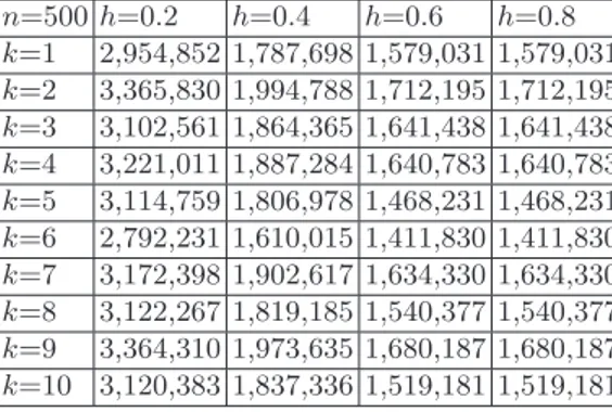
period of running without improving objective function [13]. To verify the effectiveness of the proposed algorithm, the problem sets are taken from [1,13]. The numbers of jobsnare set to 50, 100, 200, 500 and 1000, and four restrictive factors h = 0.2, 0.4, 0.6, and 0.8 are used to determine the common due date defined asd=⌊hPi⌋. For each combination ofnandh, ten problems represented thek−th instance of a combination are used for testing. Tables 4.1 to 4.5 tabulate all simulation results for the proposed algorithm.

Table 4.1: Simulation results ofn_{=50 for the proposed algorithm.} n₌₅₀h_=0.2 h_=0.4 h_=0.6 h_=0.8

k_{=1 40,697 23,792 17,969 17,934} k_{=2 30,613 17,907 14,050 14,040} k_{=3 34,425 20,500 16,497 16,497} k_{=4 27,755 16,657 14,080 14,080} k_{=5 32,307 18,007 14,605 14,605} k_{=6 34,969 20,385 14,251 14,066} k_{=7 43,134 23,038 17,616 17,616} k_{=8 43,839 24,888 21,329 21,329} k_{=9 34,228 19,984 14,202 13,942} k_{=10 32,958 19,167 14,366 14,363}

Table 4.2: Simulation results ofn_{=100 for the proposed algorithm.} n=100 h=0.2 h=0.4 h=0.6 h=0.8

k=1 145,516 85,884 72,017 72,017

k=2 124,916 72,982 59,230 59,230

k_{=3 129,800 79,598 68,537 68,537} k_{=4 129,584 79,405 68,759 68,759} k_{=5 124,351 71,275 55,286 55,103} k_{=6 139,188 77,778 62,398 62,398} k_{=7 135,026 78,244 62,197 62,197} k_{=8 160,147 94,365 80,708 80,708} k_{=9 116,522 69,457 58,727 58,727} k_{=10 118,911 71,850 61,361 61,361}

To show the superiority of the proposed algorithm, the percentage im-provement of the obtained values (FOB_{) for the proposed algorithm and}

var-ious approaches were compared with regard to the benchmarks, provided by Biskup and Feldman (FBF_{), which can be calculated as follows [1, 13]:}

Improvement rate (IR) =F

BF _−FOB

Table 4.3: Simulation results ofn_{=200 for the proposed algorithm.} n=200 h=0.2 h=0.4 h=0.6 h=0.8

k=1 498,653 295,684 254,259 254,259

k_{=2 541,180 319,199 266,002 266,002} k_{=3 488,665 293,886 254,476 254,476} k_{=4 586,257 353,034 297,109 297,109} k_{=5 513,217 304,662 260,278 260,278} k_{=6 478,019 279,920 235,702 235,702} k_{=7 454,757 275,017 246,307 246,307} k_{=8 494,276 279,172 225,215 225,215} k_{=9 529,275 310,400 254,637 254,637} k_{=10 538,332 323,077 268,353 268,353}

Table 4.4: Simulation results ofn_{=500 for the proposed algorithm.}

n₌₅₀₀ h_=0.2 h_=0.4 h_=0.6 h_=0.8

k_{=1 2,954,852 1,787,698 1,579,031 1,579,031} k_{=2 3,365,830 1,994,788 1,712,195 1,712,195} k_{=3 3,102,561 1,864,365 1,641,438 1,641,438}

k=4 3,221,011 1,887,284 1,640,783 1,640,783

k=5 3,114,759 1,806,978 1,468,231 1,468,231

k=6 2,792,231 1,610,015 1,411,830 1,411,830

k=7 3,172,398 1,902,617 1,634,330 1,634,330

k_{=8 3,122,267 1,819,185 1,540,377 1,540,377} k_{=9 3,364,310 1,973,635 1,680,187 1,680,187} k_{=10 3,120,383 1,837,336 1,519,181 1,519,181}

Table 4.5: Simulation results ofn_{=1000 for the proposed algorithm.} n₌₁₀₀₀ h_=0.2 h_=0.4 h_=0.6 h_=0.8

k_{=1 14,054,929 8,110,906 6,410,875 6,410,875} k_{=2 12,295,998 7,271,371 6,110,091 6,110,091} k_{=3 11,967,290 6,986,816 5,983,303 5,983,303} k_{=4 11,796,599 7,024,050 6,085,846 6,085,849} k_{=5 12,449,588 7,364,810 6,341,477 6,341,477} k_{=6 11,644,121 6,927,585 6,078,373 6,078,375} k_{=7 13,277,006 7,861,297 6,574,297 6,574,297} k_{=8 12,274,736 7,222,137 6,067,312 6,067,312}

k=9 11,757,063 7,058,786 6,185,321 6,185,321

100 Lee, Lin and Ying

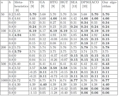
The averaged improvement rate of the proposed algorithm and various approaches over the benchmarks are shown in Table 4.6. In Table 4.6, each cell represents the averaged value of ten instances (k= 1,2, . . . ,10), and the best results in the literature are reported in bold. It shows that the proposed algorithm has the best performance among these compared approaches except forn=200 andh=0.4. We noted that the proposed algorithm is also superior to ACO as shown in Table 4.6.

Table 4.6: The averaged improvement rate of the proposed algorithm and various approaches.

n h

Meta-heuristics [6]

TS [9]

GA [9]

HTG [9]

HGT [9]

SEA [13]

DPSO [33]

ACO Our algo-rithm

50 0.2 5.65 5.70 _5.68 5.70 5.70 5.58 5.68 5.70 5.70

0.4 4.64 4.66 4.60 4.66 4.66 4.42 4.66 4.66 4.66

0.6 0 0.32 0.31 0.27 0.31 0.31 0.34 0.33 0.34

0.8 0 0.24 0.19 0.23 0.23 0.24 0.24 0.24 0.24

100 0.2 6.18 6.19 6.17 6.19 6.19 6.12 6.19 6.19 6.19

0.44.94 4.93 4.91 4.93 4.93 4.85 4.94 4.92 4.94

0.6 0 0.01 0.12 -0.08 -0.04 0.14 0.15 0.15 0.15

0.8 0 0.15 0.12 0.08 0.11 0.17 0.18 0.17 0.18

200 0.2 5.73 5.76 5.74 5.76 5.76 5.75 5.78 5.76 5.78

0.43.79 3.74 3.75 3.75 3.75 3.72 3.74 3.75 3.75

0.6 0 0.01 0.13 -0.37 -0.07 0.15 0.15 0.15 0.15

0.8 0 0.04 0.14 -0.26 -0.07 0.15 0.15 0.15 0.15

500 0.2 6.40 6.41 6.41 6.41 6.41 6.42 6.42 6.42 6.43

0.4 3.52 3.57 3.58 3.58 3.58 3.56 3.56 3.57 3.58

0.6 0 -0.25 0.11 -0.73 -0.15 0.11 0.11 0.11 0.11

0.8 0 -0.21 0.11 -0.73 -0.13 0.11 0.11 0.11 0.11

1000 0.2 6.72 6.73 6.75 6.74 6.74 6.77 6.76 6.76 6.77

0.4 4.30 4.39 4.40 4.39 4.39 4.39 4.38 4.38 4.40

0.6 0 -1.01 0.05 -1.28 -0.42 0.05 0.06 0.06 0.06

0.8 0 -1.13 0.05 -1.28 -0.40 0.05 0.06 0.06 0.06

4.6 Conclusions

4 ACO with Heuristics for Scheduling on a Single Machine 101

of heuristic information. Furthermore, heuristics are embedded into the pro-posed algorithm to ameliorate its search performance. We use the benchmarks, provided by Biskup and Feldman, to test the performance of the proposed al-gorithm. From simulation results, it indicates that the proposed algorithm outperforms original ACO and other approaches.

References

1. Biskup, D. and Feldmann, M. (2001) Benchmarks for scheduling on a single machine against restrictive and unrestrictive common due dates, Computers and Operations Research: 28(8) 787-801.

2. Garey, M. and Johnson, D. (1979). Computers and Intractability: A Guide to the Theory of NP Completeness, W. H. Freeman and Company, San Francisco, California.

3. Bose, R. (2002) Information theory, coding, and cryptography, McGraw Hill. 4. Gordon, V., Proth, J.-M. and Chu, C. (2002) A survey of the state-of-art of

common due date assignment and scheduling research, European Journal of Operational Research: 139(1) 1-25.

5. Gupta, J. N. D., Lauff, V. and Wernerm F. (2004) Two-machine flow shop problems with nonregular criteria, Journal of Mathematical Modelling and Algorithms: 3 123-151.

6. Feldmann, M. and Biskup D. (2003) Single-machine scheduling for minimizing earliness and tardiness penalties by meta-heuristic approaches, Computers and Industrial Engineering: 44(2) 307-323.

7. James, R. J. W. (1997) Using tabu search to solve the common due date early/tardy machine scheduling problem, Computers and Operations Research: 24(3) 199-208.

8. Hall, N. G., Kubiak, W. and Sethi, S. P. (1991) Earliness-tardiness scheduling problem, II: deviation of completion times about a restrictive common due date, Operations Research: 39(5) 847-856.

9. Hino, C. M., Ronconi, D. P., and Mendes, A. B. (2005) Minimizing earliness and tardiness penalties in a single-machine problem with a common due date, European Journal of Operational Research: 160(1) 190-201.

10. Hoogeveen, J. A. and Velde Van De S. L. (1991) Scheduling around a small common due date, European Journal and Operational Research: 55(2) 237-242. 11. Liaw, C.-F. (1999) A Branch-and-Bound Algorithm for the Single Machine Earliness and Tardiness Scheduling Problem, Computers and Operations Re-search: 26 679-693.

12. Mondal, S. A. and Sen, A. K. (2001) Single machine weighted earliness– tardiness penalty problem with a common due date, Computers and Oper-ations Research: 28 649-669.

13. Lin, S.-W., Chou, S.-Y., and Ying, K.-C. (2007) A sequential exchange ap-proach for minimizing earliness-tardiness penalties of single-machine schedul-ing with a common due date, European Journal of Operational Search: 177 1294-1301.

102 Lee, Lin and Ying

15. Lee, Z.-J., Lee, C.-Y. (2005) A Hybrid Search Algorithm with Heuristics for Resource Allocation Problem, Information sciences: 173 155-167.

16. Mittenthal, J., M. Raghavachari, and A. I. Rana. (1993) A hybrid simulated annealing approach for single machine scheduling problems with non-regular penalty functions, Computers and Operations Research: 20 103-111.

17. Lee, C. Y. and Kim, S. J. (1995) Parallel genetic algorithms for the earliness-tardiness job scheduling problem with general penalty weights, Computers and Industrial Engineering: 28(2) 231-243.

18. Liu, M. and Wu, M. (2006) Genetic algorithm for the optimal common due date assignment and the optimal policy in parallel machine earliness/tardiness scheduling problems, Robotics and Computer-Integrated Manufacturing: 22 279-287.

19. Jaynes, E. T. (1982) On the rationale of the maximum entropy methods. Pro-ceedings of the IEEE: 70(9) 939-952.

20. Kahlbacher, H. G. (1993) Scheduling with monotonous earliness and tardiness penalties, European Journal of Operational Research: 64(2) 258-277.

21. Raghavachari, M. (1988) Scheduling problems with non-regular penalty func-tions: a review, Operations Research: 25 144-164.

22. Szwarc, W. (1989) Single-machine scheduling to minimize absolute deviation of completion times from a common due date, Naval Research Logistics: 36 663-673.

23. Smith, W. E. (1956) Various optimizers for single-stage production, Naval Re-search Logistics Quarterly: 3 59-66.

24. Dorigo M. and St¨utzle T. (2004). Ant Colony Optimization: The MIT Press. 25. Lee, C.-Y., Lee, Z.-J. and Su, S.-F. (2005) Ant Colonies With Cooperative

Process Applied To Resource Allocation Problem, Journal of the Chinese In-stitute of Engineers: 28 879-885.

26. Lee, Z.-J., Lee, C.-Y. and Su, S.-F. (2002) An Immunity Based Ant Colony Optimization Algorithm for Solving Weapon-Target Assignment Problem, Ap-plied Soft Computing 2(1) 39-47.

27. Lee, Z.-J. and Lee, W.-L. (2003) A Hybrid Search Algorithm of Ant Colony Optimization and Genetic Algorithm Applied to Weapon-Target Assignment Problems, Lecture Notes in Computer Science 2690: 278-285.

28. Bauer, A. et al. (1999) An ant colony optimization approach for the single machine total tardiness problem, Proceedings of the 1999 Congress on Evolu-tionary Computation: 2 1445-1450.

29. Varela, G. N. and Sinclair, M. C. (1999) Ant colony optimization for virtual wavelength path routing and wavelength allocation, Proceedings of the 1999 Congress on Evolutionary Computation: 3 1809-1816.

30. Dicaro, G. and Dorigo, M. (1998) Mobile agents for adaptive routing, Proceed-ings of the Thirty-First Hawaii International Conference on System Sciences: 7 74-83.

31. Yu, I. K., Chou, C. S. and Song,Y. H. (1998) Application of the ant colony search algorithm to short-term generation scheduling problem of thermal units, Proceedings of the 1998 International Conference on Power System Technology: 1 552-556.

4 ACO with Heuristics for Scheduling on a Single Machine 103