A MULTICRITERIA PERMUTATION FLOWSHOP SCHEDULING PROBLEM WITH SETUP TIMES

(1)

A MULTICRITERIA PERMUTATION

FLOWSHOP SCHEDULING PROBLEM

WITH SETUP TIMES

M.Saravanan#1, S.Joseph Dominic Vijayakumar#2, R.Srinivasan

*

#3 1

Principal, Sri Subramanya College of Engineering & Technology, Palani, India. 2

Assistant Professor, 3 Associate Professor, RVS College of Engineering & Technology, Dinidgul, India 1

drmsaravanan@yahoo.com, 2joedominic_s@yahoo.co.in, 3

Abstract: The permutation flow shop scheduling problem has been completely concentrated on in late

decades, both from single objective and additionally from multi-objective points of view. To the best of our information, little has been carried out with respect to the multi-objective flow shop with sequence dependent setup times are acknowledged. As setup times and multi-criteria problems are significant in industry, we must concentrate on this area. We propose a simple and powerful meta-heuristic algorithm as artificial immune system for the sequence dependent setup time’s flow shop problem with several criteria. The objective functions are framed to simultaneously minimize the makespan time, tardiness time, earliness time and total completion time. The proposed approach is in conjunction with the constructive heuristic of Nawaz et al. evaluated using benchmark problems taken from Taillard and compared with the prevailing Simulated annealing approach and B-Grasp approach. Computational experiments indicate that the proposed algorithm is better than the SA approach and B-Grasp approach in all cases and can be very well applied to find better schedule.

sriparam_2000@yahoo.com

Keywords: Permutation flow shop scheduling, Makespan, Tardiness, Earliness, Total completion time,

Simulated annealing algorithm, B-Grasp approach, Artificial Immune System algorithm. I. INTRODUCTION

Scheduling is a standout amongst the most essential concerns in operation research. As a typical manufacturing and scheduling problem with strong industrial background, flow shop scheduling with limited buffers has offered wide consideration both in academic and engineering fields. Flow shop scheduling problem, or FSP, is a class of group shop scheduling problems in which the operations of each job must be processed on machines 1, 2, …, m in this same order. A special case of FSP is permutation flow shop scheduling problem, in which the processing order of the jobs on the machines is the same for each machine. Early research on flow shop problems was primarily dependent upon the Johnson's approach, which gives a proper strategy to place an optimal solution with two or three machines with specific attributes [1, 2]. Johnson described an exact approach to minimize makespan for the n-jobs and 2-machines ﬂow shop scheduling problem. The point when the ﬂow shop scheduling problem broadens as including more jobs and machines, it turns into a combinatorial optimization problem. It is clear that combinatorial optimization problems are in NP-hard problem class, and near optimal solution strategies are favoured for such problems.

Another area of research in the scheduling includes the multi-criteria problem. The majority of examination on scheduling problems addresses just a single criterion while the majority of real-life problems require the decision maker to think about more than a single criterion before arriving at a decision. Multiple objectives make the flow shop show more complicated, however closer to real application. [3].In the case of multi-objective FSP, the completion of getting non-dominated results needs to think about the evaluation of a few unique objectives. Therefore, MFSP is more impulsive than single goal FSP and needs to expend more perverse computational time. At present, a large portion of the literary works kept tabs on the feasibility of the algorithm and ignored computational productivity.

The criteria scheduling problems are classified into three classes. In the first class, one of the multi-criteria is acknowledged as the objective to be optimized while the other is recognized as a constraint. In the second one, both criteria are acknowledged similarly important and the problem includes discovering effective schedules. In the third one, both criteria are weighted contrastingly and an objective function as the sum of weighted functions is defined. The problem recognized in this paper has a place with the third class.

(2)

conceivable to ignore them. Scheduling problems including setup times might be divided into two classes, the

ﬁrst class is sequence independent and the second is dependent setup times. Setup is dependent, if its duration depends on both the current and the immediate preceding job and is sequence-independent if its duration depends only on the current job to be processed [4–10].

Sequence-dependent setup times are typically found in the situation where the facility is a multipurpose machine. A few samples of sequence-dependent setups include (i) manufacturing of chemical compounds, where the degree of the cleaning depends on both the chemical most recently processed and the chemical about to be processed and (ii) in the printing industry, the cleaning and setting of the presses for processing the next job depends on its difference from the ink colour, paper size and types used in the earlier job. The case of sequence-dependent setups could be found in various other industrial systems, which include the stamping operation in plastic manufacturing, die changing a metal processing shop, and roll slitting in the paper industry [4]. A recent survey of scheduling research involving setup times is given by [4 -7].

The makespan criterion is a production-oriented performance measure. The majority of the scheduling literature has concentrated bi-criteria problems such as makespan and flow time and are related to productivity and facility utilization [11-14]. The main second criterion is the minimization of the total completion time. The performance measure of total completion time is very important as it is directly related to the cost of inventory. In the modern manufacturing environment, customer satisfaction is an important issue and henceforth on-time delivery turns into an important factor to get by in a competitive market. In this perspective scheduling is to be successful not just in the part of productivity and facility utilization additionally to meet the customer expectations. The job not finished till its due date can result in unhappiness the customer. Consequently due date related measures must be incorporated in the scheduling issue. On the other hand, if work is finished prior than the due date, an inventory expense is charged till the due date. To meet these two objectives, it is important that all the jobs should be finished on their allotted due dates as careful as could be expected under the circumstances [15]. Few of the researchers consider the due date related criteria and model the problem as tri-criteria problem [16 – 20].

Artificial immune system is a current and buoyant meta-heuristic algorithm for combinatorial optimization problems. Some researchers have focused on applying AIS to various scheduling problems like flow shop scheduling problem [21], the job shop scheduling problem [22, 23, 24], the hybrid flow scheduling problem [25] and the multiprocessor scheduling problem [26, 27]. In view of the fact that, Earliness/ Tardiness (E/T) is an important determination in due date associated problems. In this paper, a multi-criteria scheduling problem with separate setup times on permutation flow shop is taken for consideration. The objective function of the problem is to minimize the weighted sum of total completion time, makespan, maximum tardiness and maximum earliness. To the best of our knowledge this is the first study that addresses AIS algorithm to minimize the above said objective function.

II. PROBLEM DESCRIPTION

The objective of this work is to determine the optimal schedule that minimizes four performance measures such as minimizing weighted sum of total completion time, makespan, tardiness and earliness. The makespan (Cmax), defined as max (C1……. Cn) is equivalent to the completion time of the last job to leave the system. Total tardiness (Tj) is a due date related performance measure and it is considered as summation of tardiness of individual jobs, where Tj= Cj – dj. Total earliness (Ej) is also a due date related performance measure but reflects early delivery of jobs and it is considered as summation of earliness of individual jobs, where, Ej= Cj – dj

Where, λ

and ∑C is the total completion time. Therefore, the formulation of the multi-criteria objective function is framed as

��1��+ �2� ��

�=1

+ �₃� �_� �

�=1

+ �₄� � �

�=1

��. 1

1+ λ2+ λ3+λ4

Let

=1.

i Machine j Job

m Number of machines n Number of jobs Cj

d

Completion time of job j

j

λ

Due date of job j

1 Weight for the Makespan, 0 ≤ λ1

λ

≤ 1

(3)

λ3 Weight for the maximum earliness, 0 ≤ λ3

λ

≤ 1

4 Weight for the total completion time, 0 ≤ λ4

III. SIMULATED ANNEALING APPROACH

≤ 1

Simulated annealing approach (SAA) is so named due to its analogy to the process of physical annealing with solids, in which a crystalline solid is warmed and then permitted to cool gradually until it attains its most normal possible crystal lattice configuration (i.e., its minimum lattice energy state), and along these lines is free of crystal defects. Assuming that the cooling schedule is sufficiently moderate, the final configuration brings about a solid with such superior structural integrity. Simulated annealing establishes the connection between this kind of thermodynamic behaviour and the search for global minima for a discrete optimization problem. Furthermore, it gives an algorithmic intends to exploiting such a connection. Recreated annealing is introduced to combinational optimization by Kirkpatrick [28] in 1982.

Simulated annealing is a neighbourhood searching methodology intended to obtain a global ideal solution for combinatorial optimization problems. It begins with an initial solution and iteratively moves towards the other existing solutions, while remembering the best solution discovered in this way. In order to diminish the probability of getting trapped in nearby optima, simulated annealing acknowledges the moves even around the inferior neighbouring solutions under the control of randomized scheme. More accurately, if a move from current solution S to another inferior neighbouring solution S* brings about a change ΔE = f(s')-f(s) in the objective ΔE function value, the move is still acknowledged if R <exp(-ΔE/T)

IV. B–GRASP APPROACH

where T is a control parameter, called temperature, and R is an uniform random number between interval (0, 1). Initially, the temperature T is sufficiently high permitting numerous deteriorative moves to be acknowledged, and then it is brought down at a low speed of rate to the point which the inferior moves are more or less rejected. This algorithm examines successfully and steadily the probable neighbors, in each temperature, in order to achieve the best result.

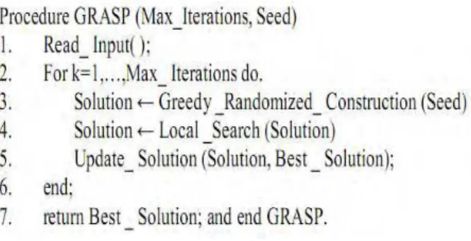
The GRASP (Greedy Randomized Adaptive Search Procedure) meta-heuristic [29, 30] is a multi-start or iterative process. Basically it consists of two phases: construction and local search. The construction phase fabricates a feasible solution, whose neighbourhood is researched until a local minimum is found throughout the local search phase. The best general solution is kept as the result. A far reaching review of the literature is given in [31]. The pseudo-code for grasp Figure 1, outlines the main blocks of a GRASP methodology for minimization, in which Max Iterations are performed and Seed is utilized as the initial seed for the pseudo random number generator.

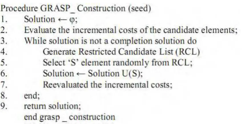
Figure 2, illustrates the construction phase with its pseudo-code. Each iteration of this phase let the set of candidate elements be formed by all elements that can be incorporated to the partial solution under construction without destroying feasibility. The selection of the next element for incorporation is determined by the evaluation of all candidate elements according to a greedy evaluation function.

Fig 1. Pseudo – code for GRASP

(4)

Fig 2. Pseudo –code of GRASP Construction phase

The solutions created by a greedy randomized construction are not so much optimal, even concerning basic neighborhoods. The local search stage generally enhances the constructed solution. A local search algorithm works in an iterative fashion by successively replacing the current solution by a better solution in the neighborhood of the current solution. It ends when no better solution is found in the neighborhood. The pseudo-code of a fundamental local search algorithm is beginning of the solution developed in the first stage and utilizing a neighborhood. The effectiveness of a local search procedure based on several aspects, such as the neighborhood structure, the neighborhood search technique, the fast evaluation of the cost function of the neighbors, and the starting solution itself. The construction phase assumes an extremely essential part regarding this last aspect, building high-quality starting solutions for the local search. Basic neighborhoods are normally utilized. The neighborhood search may be done by either best improving or a first-improving strategy. On account of the best improving technique, all neighbors are explored and the current solution is replaced by the best neighbor. In the case of a first-improving strategy, the current solution moves to the first neighbor whose cost function value is smaller than that of the current solution. Generally, both methodologies lead to the same final solution, the first-improving strategy is used having smaller computational time. We also found that premature convergence to a non-global local minimum is more likely to occur with a best-improving strategy.

V. ARTIFICIAL IMMUNE SYSTEM

Artificial immune system (AIS) is a meta-heuristic approach based on the principle of the biological immune system. Artificial immune systems applications include the following areas: clustering and classification [33], anomaly detection [34], optimization [35], control [36], computer security, learning, bioinformatics, image processing, robotics, virus scanning and web mining [37], and scheduling [38]. Clonal selection is the base of the immune algorithms. The clonal selection principle uses the immune system to express the basic features of an immune response to antigens. The idea is that only cells that recognize antigens proliferate should be selected. The process of proliferation is called clonal expansion. Then the selected cells are subjected to an Affinity maturation process which develops its affinity to selective antigens. In the field of optimization, the first algorithm proposed by clonal selection called CLONALG.

The first algorithm was proposed by clonal selection called CLONALG and used for optimization. Other versions of the clonal selection algorithm have been designed to improve the performance of CLONALG. This section describes the proposed method that has been utilized to solve the two-stage multi-machine assembly scheduling problem. In the next subsections, we start by identify the representation of the solution, the mechanisms used to generate the initial solution, and how AIS has been adapted to improve the initial solutions.

The antibody (candidate solution) is encoded by a string of integers. The string implies the order of the jobs to be processed. Cell indexes of the string represent the order of the job sequence to be processed and each string value indicates the job location.

In the initialization stage, the algorithm parameters such as the size of the population, the number of iterations and stopping criteria are considered. The initial population (P) is nothing but is randomly generated number of solutions (antibodies). The objective value (fitness function) for each antibody is calculated.

A. Clonal Selection

Each antibody will be cloned in the population is proportional to its affinity to generate the population (PC). The affinity of each antibody can be calculated by equation 2.

��=�1_�_{��}_{��}� ��. 2

(5)

calculate the number of clones to be generated for each antibody. B. Mutation

Each clone in the population (PC) is mutated to generate a new another population (Pm). It can be done by swapping (pairwise, inverse) two random job cells of the clone. The probability of applying the mutation operator is calculated by using the equation 3.

∝ = �−�� . 3

Where, α is the probability of applying a mutation mechanism.

After the mutation process the population (pm) is combined with the initial population (P) to generate another population (Px). The antibodies in the new population (Pn) are listed in descending order based on their affinity values and select the antibodies having higher affinity values to generate new population (Pn). Then the lowest L antibodies in the new population (Px) are replaced and same number of L antibodies are randomly generated. The pseudo code for the proposed AIS based algorithm is given in figure 3.

Fig 3. Pseudo – code of AIS algorithm

VI. COMPUTATIONAL RESULTS AND COMPARISONS

In this section, the results of computational tests associated with the AIS algorithm are presented. The coding of the proposed algorithm is programmed in JAVA and implemented on a personal computer with Dual Core and 2GB RAM.

To test the performance of the AIS, benchmark problems proposed by Taillard [39] are selected. Six hundred problem instances with the number of machines ranging from 5 to 20, number of jobs ranging from 20 to 200 and Weightage factor ranges from (0.1, 0.1, 0.1,0.7), (0.1,0.1,0.7,0.1), (0.1,0.7,0.1,0.1), (0.7,0.1,0.1,0.1) and (0.25,0.25,0.25,0.25) have been generated. Twelve different sized benchmark problems (20 × 5, 20 × 10, 20 × 20, 50 × 5, 50 × 10, 50 ×20, 100 × 5, 100 × 10, 100 × 20, 200 × 5, 200 × 10, 200 × 20) each with 10 different instances were considered. The jobs due dates are randomly generated in the range from equation 4.

��= ��+� ��+� (� −1) �

�=1

�� . 4

Where��_��, represents the average setup time, p_jis the average processing time of job ‘j’ and n indicates the

number of jobs to be processed and ‘u’ is a random number between zero and one. The average setup time of a job is double the mean processing times of job.

The Relative percentage deviation (RPD) is taken as a performance measure for comparison and given in equation 5, [40]. The performance of AIS is compared with B-GRASP and SAA.

��= (100∗(�� − ��)

�� . (5)

(6)

TABLE I

Relative Performance Deviation (sec) for Weightage Factor (0.1, 0.1, 0.1, 0.7)

AIS B-GRASP CRH

n M AVG MAX AVG MAX AVG MAX

20

5 0.078290695 0.782906946 0.59475155 1.008802884 3.959188757 1.329245599

10 0.147823349 1.141842407 0.70108581 1.760765128 3.359564732 5.752288158

20 0.399833377 1.660653804 0.35017615 1.051046958 2.833578654 4.657712545

50

5 0.042354689 0.658985646 0.68254236 0.25365657 4.860588877 9.104824294

10 0.072543216 1.124568979 0.985426125 0.356985656 1.742419721 3.386115434

20 0.106212731 0.995608361 1.22154879 0.568956324 0.966059586 2.8513141

100

5 0.08562354 1.25456989 1.769831696 2.29656147 1.387884207 7.115493099

10 0.171861367 0.783053358 1.599837699 3.154100548 2.419708719 1.336521236

20 1.048879849 2.022179155 3.33902483 2.166198137 3.685691625 1.747215614

200

5 1.112546879 0.655689786 1.965234724 0.698562312 2.542653256 1.325456988

10 1.68545897 0.985621547 2.356245873 0.985645659 2.985645236 1.451256321

20 1.98564875 0.995689563 3.754286957 1.123565659 4.213564876 1.658985623

n = number of jobs; m= number of machines; Relative Performance Deviation in terms of seconds

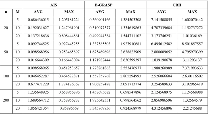
TABLEII

20

5 0.686436015 1.205181224 0.360901166 1.384503308 7.141508055 1.602070442

10 0.192031627 1.247961901 0.510077377 1.334619863 4.707339684 1.152737272

20 0.137218636 0.808444861 0.499944384 1.544711102 3.173746251 1.01036169

50

5 0.092744525 0.927445255 1.337585503 1.927910681 6.495612582 8.501857557

10 0.098568956 0.253465897 1.675469698 2.638823909 2.800609652 4.795970399

20 0.016644309 0.166443094 1.171982444 2.630599397 1.839190678 3.11293137

100

5 0.098568965 0.451253657 1.778261863 2.553476977 1.988260989 7.371993633

10 0.046452287 0.464522871 1.557857768 2.805294993 2.526066604 2.630116502

20 0.677471229 1.774126362 1.906257478 3.091713774 3.254589633 3.192965419

200

5 1.235648925 0.658956896 1.458695682 0.698547896 2.124568975 1.124568988

10 1.689564712 0.758956237 1.985642351 0.798564562 2.856986596 1.32564579

(7)

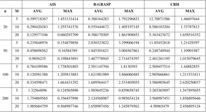
TABLE III

20

5 0.399718367 1.453131414 0.388164283 1.792296823 12.70071586 1.46697644

10 0.290420283 1.255741576 0.555444672 1.405197145 8.586103204 1.33787813

20 0.129577106 0.660293709 0.388170305 1.861908852 5.363423672 1.658516352

50

5 0.235648976 0.154879856 2.030323822 3.299006194 11.85452818 1.21429397

10 0.458698562 0.16584789 1.845301621 3.004567861 6.248740944 1.10901987

20 0.9856235 0.198843891 1.467778945 2.714474397 2.401261195 1.015079645

100

5 0.784109586 1.738501803 2.501145704 1.8130393 2.569457514 1.44882855

10 0.120581388 1.205813883 1.621981989 3.866060485 2.985666861 1.211533411

20 0.334598471 1.661631292 1.689564417 2.533405055 3.586985645 2.620250037

200

5 1.32564896 0.124565896 1.985645236 0.859658745 3.265365897 1.547895655

10 1.754869565 0.356457896 2.124568987 0.985654124 3.568987451 1.856895646

20 1.985684759 0.568987746 2.658987456 1.245879562 4.58965479 2.456895124

TABLE IV

20

5 0.178903063 0.723961136 0.353993284 1.027292364 3.205708105 6.052747595

10 0.483395996 1.113051986 0.360148567 1.746153371 2.406922637 4.361188764

20 0.934324637 1.364001102 0.446556626 1.99486714 3.576508031 3.06337085

50

5 0.985658746 0.125478954 1.304290461 2.042155899 2.009618886 2.62894933

10 0.427072143 1.146731255 1.351935934 2.628251011 1.558693557 4.019128508

20 0.507107379 1.686459289 1.494738366 2.848096781 1.886976658 2.799980536

100

5 0.856985648 0.214587964 1.537918713 2.216875729 4.146027791 7.160247654

10 0.01466572 0.146657202 1.214187841 2.04235765 1.102835726 2.245080513

20 1.164854471 2.160319931 2.582903157 3.191678894 1.035447855 0.354478549

200

5 1.456985623 0.56895479 1.589685655 0.874562315 2.214568963 0.98956899

10 1.89568749 0.658974562 1.985658976 0.985658956 3.124587963 1.256547896

(8)

TABLE V

20

5 0.363702124 1.167571327 0.300743755 1.311346202 5.203335614 7.051077838

10 0.166357893 0.805938965 0.542858759 2.271840856 3.339526911 6.479206319

20 0.498007931 1.385381717 0.112905677 0.891805687 3.067941635 4.81357058

50

5 0.014025237 0.140252366 1.445322017 2.786282992 5.964068996 8.083665875

10 0.785658957 0.39481007 0.923394275 2.483863656 6.32212336 1.75236302

20 0.116893261 0.856304431 1.170184132 2.372402429 1.212474855 3.303655244

100

5 0.213456796 0.10214563 1.946446383 3.071754264 4.905217754 7.571290349

10 0.019801666 0.198016659 1.997748756 3.818463722 1.301435214 3.210687597

20 0.630301093 1.301504919 2.126109177 2.878742944 1.058406956 1.30180075

200

5 1.356987895 0.854758966 1.985698562 2.5246589 2.568974563 1.124578966

10 1.789652365 0.98564759 2.124568979 1.021457896 2.98563266 1.456895652

20 1.989856322 1.124574125 2.658974561 1.214587965 3.456897564 1.98564759

(9)

Fig5. Average percentage error versus number of jobs for (0.1, 0.1, 0.7, 0.1)

(10)

VII. CONCLUSION

(11)

REFERENCES

[1] Johnson, S.M, “Optimal two- and three-stage production schedules with setup times included,” Naval Research Logistics Quarterly, (1), 61–68, 1954.

[2] Kamburowski, J, “The nature of simplicity of Johnson’s algorithm,” Omega – International Journal of Management Science, (25), 581–584, 1997.

[3] Yagmahan B, Yenisey MM., “A multi-objective ant colony system algorithm for flow shop scheduling problem,” Expert Syst. Appl. 37, 1361–1368, 2010.

[4] Wen – Hwa Yang, “Survey of scheduling research involving setup times,” International Journal of Systems Scien

[5] T.C.E.Cheng, J.N.D.Gupta, and G.Wang, “A review of ﬂowshop scheduling research with setup times,” Product operations Management, 9 (3), 262–282, 2000.

[6] A.Allahverdi, J.N.D.Gupta, and T.Aldowaisan, “A review of scheduling research involving setup considerations,” Omega, 27, 219– 239, 1999.

[7] A.Allahverdi, C.T. Ng, T.C.E. Cheng, and M.Y. Kovalyov, “A survey of scheduling problems with setup times or costs,” European Journal f Operational Research, 187(3), 985– 1032, 2008.

[8] T.Eren, E.Guner, “A bicriteria ﬂowshop scheduling problem with setup times,” Applied Mathematics and Computation, 183 (2), 2006. [9] T.Eren, “A multicriteria scheduling with sequence-dependent setup times,” Applied Mathematical Sciences,1(58), 2883–2894, 2007. [10] T. Eren, “The solution approaches for multicriteria ﬂowshop scheduling problems,” Ph.D. thesis, Gazi University Institute of Science

and Technology Ankara, Turkey, 2004.

[11] Shih-Wei Lin, Kuo-Ching Ying,

[12] T. Pasupathy, Chandrasekharan Rajendran and R.K. Suresh, “A multi-objective genetic algorithm for scheduling in flow shops to

minimize makespan and total flow time,” International Journal of Advanced Manufacturing Technology, Springer-Verlag London Ltd, 27, 804-815, 2006.

[13] D. Ravindran, A.NoorulHaq, S.J.Selvakumar and R. Sivaraman, “Flow shop scheduling with multiple objective of minimizing makespan and total flow time,” International Journal of Advanced Manufacturing Technology, 25, 1007–1012, 2005.

[14] B. Yagmahan B, MM. Yenisey, “A multi-objective ant colony system algorithm for flow shop scheduling problem,” Expert Syst.Appl. 37, 1361– 1368, 2010.

[15] C.S.Sung, J.I. Min, “Theory and methodology scheduling in a two machine flow shop with batch processing machine(s) for earliness measure under a common due date,” European Journal of Operational Research, 131, 95-106, 2001.

[16] C.Rajendran, “Theory and methodology heuristics for scheduling in flow shop with multiple objectives,” European Journal of Operation Research, 82 (3), 540 −555, 1995.

[17] Yagmahan, B. and Yenisey, M.M., “Ant colony optimization for multi-objective flow shop scheduling problem,” Computers and Industrial Engineering, 54(3), 411-420, 2008.

[18] S.G.Ponnambalam, H.Jagannathan, M.Kataria, and A.Gadicherla, “A TSP-GA multi- objective algorithm for flow shop scheduling,” International Journal of Advanced Manufacturing Technology, 23,909–915, 2004.

[19] Sha DY, Lin HH, “A particle swarm optimization for multi-objective flow shop scheduling,” International Journal of Advanced Manufacturing Technology, 45,749–758, 2009.

[20] T. Eren, E. Guner, “The tri criteria flow shop scheduling problem”, International Journal of Advanced Manufacturing Technology,36, 1210–1220, 2008.

[21] O.Engin, A. Doyen, “A new approach to solve flow shop scheduling problems by artificial immune systems,” Journal of the Dogus University, 8, 1, pp.12–27, 2007.

[22] C.A.C. Coello, D.C. Rivera, and N.C. Cortes., Use of an artificial immune system for job shop scheduling, artificial immune systems, proceedings Lecture notes in computer science, 2787, pp.1–10, 2003.

[23] H.W. Ge, L. Sun, and Y.C. Liang,., Solving job shop scheduling problems by a novel artificial immune system, Lecture Notes in Artificial Intelligence,” 3809, pp. 839–842, 2005.

[24] M.Chandrasekaran, P. Asokan, S. Kumanan, T.Balamurugan, and S. Nickolas, “Solving job shop scheduling problems using artificial immune system,” International Journal of Advanced Manufacturing Technology, 31, pp. 580–593, 2006.

[25] O.Engin, A.Doyen, “A new approach to solve hybrid flow shop scheduling problems by artificial immune system,” Future Generation Computer Systems, 20, 6, pp.1083–1095, 2004.

[26] A.Swecicka, F.Seredynski, and A.Y. Zomaya, “Multiprocessor scheduling and rescheduling with use of cellular automata and artificial immune system support,” IEEE Transactions on Parallel and Distributed Systems, 17, 3, pp. 253–263, 2006.

[27] G. Wojtyla, K. Rzadca, and F. Seredynski, Artificial immune systems applied to multiprocessor scheduling, parallel processing and applied mathematics, Lecture Notes in Computer Science, 3911, pp. 904–911, 2006.

[28] S.Kirkpatrik, “Optimization by simulated annealing, Science 220(4598), pp. 671–680, 1983.

[29] T.A.Feo, M.G.C.Resende, “A probabilistic heuristic for a computationally difficult set covering problem,” Operation Research Letters, 8, pp. 67-71.

[30] T.A.Feo, M.G.C.Resende, “Greedy randomized adaptive search procedures,” Journal of Global Optimization, 6, 109-133, 1995. [31] P.Festa, M.G.C.Resende, “GRASP: a annotated bibliography. in C.C.Riberiro and p. Hansen, Essays and Surveys in Meta-heuristics,”

Kluwer Academic Publishers, 325-367, 2002.

[32] J.P. Hart and A.W.Shogan, “Semi-greedy heuristics: an empirical study,” Operation Research Letters, 6, pp. 107-114, 1987.

[33] [34] [35] [36] [37] [38]

[39] E.Taillard, “Benchmark for basic scheduling problems,” European Journal of Operational Research, 64, pp. 278-285, 1993.