AUTHOR QUERY FORM
Journal:
ECOENG
Please e-mail or fax your responses and any corrections to:
E-mail:
[email protected]
Article Number:
1634
Fax:
+353 6170 9272
Dear Author,
Any queries or remarks that have arisen during the processing of your manuscript are listed below and highlighted by flags
in the proof. Please check your proof carefully and mark all corrections at the appropriate place in the proof (e.g., by using
on-screen annotation in the PDF file) or compile them in a separate list.
For correction or revision of any artwork, please consult
http://www.elsevier.com/artworkinstructions.
Articles in Special Issues:
Please ensure that the words ‘this issue’ are added (in the list and text) to any references to
other articles in this Special Issue.
Uncited references:
References that occur in the reference list but not in the text – please position each reference in the
text or delete it from the list.
Missing references:
References listed below were noted in the text but are missing from the reference list – please make
the list complete or remove the references from the text.
Location in
Query / remark
article
Please insert your reply or correction at the corresponding line in the proof
Q1
Please check corresponding author and fax number.
Q2
Please check the unit in ‘3.7 mg ha-1 year-1’.
Q3
Uncited references: This section comprises references that occur in the reference list but not in the body
of the text. Please position each reference in the text or, alternatively, delete it. Any reference not dealt
with will be retained in this section. Thank you.
Electronic file usage
Sometimes we are unable to process the electronic file of your article and/or artwork. If this is the case, we have proceeded
by:
Scanning (parts of) your article
Rekeying (parts of) your article
Scanning the artwork
UNCORRECTED PROOF
Ecological Engineeringxxx (2010) xxx–xxx1
Contents lists available atScienceDirect
Ecological Engineering
j o u r n a l h o m e p a g e :w w w . e l s e v i e r . c o m / l o c a t e / e c o l e n g
Carbon allocation dynamics one decade after afforestation with
Pinus radiata
D.
Don and
Betula alba
L. under two stand densities in NW Spain
1
2
E. Fernández-Nú ˜nez, A. Rigueiro-Rodríguez, M.R. Mosquera-Losada
∗3
Crop ProductionDepartment,Escuela PolitécnicaSuperior, Campus de Lugo,University of Santiago de Compostela,27002 Lugo, Spain 4
5
a r t i c l e
i n f o
67
Article history:
8
Received 9 September 2009 9
Received in revised form 19 January 2010 10
Accepted 21 March 2010 11
Available online xxx
12
Keywords:
13
Silvopastoral systems 14
Pine
15
Birch
16
Carbon
17
Production
18
Growth
19
a b s t r a c t
Silvopastoral systems can contribute to the mitigation of climate change by functioning as sinks for greenhouse gases better than exclusively agricultural systems. Tree species, density, and an adequate management of the pasture carrying capacity contribute to the capacity of carbon sequestration. In this study, the capacities for carbon sequestration in silvopastoral systems that were established with two different forest species (Pinus radiataD. Don andBetula albaL.) and at two distinct densities (833 and 2500 trees ha−1) were evaluated. Tree, litterfall, pasture and soil carbon storage determinations were
carried out to deliver carbon sequestration in the different pools within the first11years of a plantation establishment. The results show that the global capacity for carbon sequestration in silvopastoral systems with pine canopy was higher than with birch cover. Independently of the forest species, the capacity for carbon sequestration increased when the systems were established at higher plantation densities. There were found strong differences in the relative proportions of carbon in each component of the system (litterfall, tree, pasture and soil). The soil component was found to be most important in the case of the broadleaf forest established at low density. The establishment of a silvopastoral system enhanced soil carbon storage, since afforestation was carried out, which results in a more enduring storage capacity compared with treeless areas.
© 2010 Published by Elsevier B.V.
1. Introduction
20
Carbon sequestration by forests is an important environmental 21
issue since the KyotoProtocol(article 3.3) was adopted in 1997 22
(http://unfccc.int/resource/docs/convkp/kpeng.pdf). That resolu-23
tion included the removals by sinks that result directly from 24
human-induced land use changes and forestry activities to meet the 25
Kyoto carbon emissions commitments by the involved countries 26
in the determined periods from 1990 onwards (Mosquera-Losada 27
et al., 2009). These facts make reforestation and afforestation, as 28
well as deforestation, very important for the global carbon bal-29
ance accounting of different countries. Reforestation of agricultural 30
land will not only contribute to an increase in carbon sequestra-31
tion on a global scale; it will also increase the supply of lumber, 32
reducing the need for the logging of old-growth forests that, con-33
sequently, releases high amounts of stored carbon (Nair et al., 34
2008). 35
To verify compliance with the Kyoto Protocol, it is vital to 36
measure the carbon sequestration caused by land use changes 37
∗Corresponding author. Tel.:+34 600942437; fax:+34 982285926. Q1
E-mail address:[email protected](M.R. Mosquera-Losada).
from agricultural to forestland, as well as the management of 38
these lands. Reforestation of agricultural land has recently been 39 promoted in Europe and has resulted in the reforestation of 40 more than one million hectares throughout Europe between 41 1994 and 1999 (EC, 2005), a result of the implementation of 42 Regulation No. 2082/92 (EU, 1992). The establishment of agro- 43 forestry in forestlands were promoted through direct payments 44 in the last European Union Rural Development Council Regulation 45 1698/2005 (EU, 2005), making it necessary to evaluate the gains 46 and losses of carbon caused by changes in tree biomass, pasture 47 production, soil organic matter content and livestock greenhouse 48 carbon (GHC) emissions. This also highlights the importance of 49 evaluating the balance of different alternatives of forest manage- 50 ment in different environments, as described by Gordon et al. 51
(2005). 52
Forest carbon stocks are affected by the previous land use, 53 tree species, tree density and the interaction of all these vari- 54 ables with climate (Reynolds et al., 2007).). In an agroforestry 55 system, edaphic carbon is considered the most important store 56 from a quantitative perspective (Dixon, 1995). The capacity to 57 increase the sequestration of carbon in the soil will largely 58 depend on the tree species used in reforestation and their den- 59 sity. Carbon storage in a silvopastoral system is balanced by the 60
0925-8574/$ – see front matter© 2010 Published by Elsevier B.V.
UNCORRECTED PROOF
emissions of greenhouse gases (CH4 and N2O) produced by the 61
ruminants that feed on it. The amount of greenhouse gases, here 62
called GHG emitted by livestock depends on the stocking rate, 63
which depends on pasture production that is affected by tree 64
development after afforestation. Thus, these should also be eval-65
uated. 66
Agroforestry systems are not broadly extended within the 67
Atlantic area of the European Union, where the important growth 68
of trees could improve theEuropeanunion carbon sequestration. 69
Carbon sequestration studies carried out in the Atlantic region of 70
Europe are related to grasslands or crops but not to forestlands, 71
where aspects related to above and belowground carbon seques-72
tration should be evaluated. Moreover, comparisons between tree 73
species development and densities and their effect on livestock 74
GHG emissions as well as on carbon sequestration should be car-75
ried out as pasture production and the chemical composition, and 76
the quantity and rate of incorporation of carbon to soil from lit-77
terfall depends on tree species identity and density (Prescott et 78
al., 2000). Compared with exclusively forest systems, carbon in sil-79
vopastoral systems should be evaluated. Some estimates assert that 80
livestock production accounts for 18% of climate change, produces 81
9% of CO2 emissions, 37% of CH4 emissions, and 65% of the N2O 82
(Steinfeld et al., 2006). Moreover, long term studies should be car-83
ried out to quantify global carbon sequestration as tree canopy in 84
the Atlantic region is fast developed, which affects to the global 85
system biomass production (tree, pasture and therefore livestock), 86
the inputs of organic matter into the soil and therefore the global 87
carbon sequestration in the different pools of the agroforestry sys-88
tems. 89
This paper aims to evaluate the amount of carbon sequestration 90
in two silvopastoral systems that were established at two densities 91
ofPinus radiataD. Don (pine) orBetula albaL. (birch)during the11
92
years after trees were planted. 93
2. Materials and methods
94
2.1. Characteristics of the study site 95
The experiment was conducted in Castro Riberas de Lea 96
(province of Lugo, NW Spain) at a latitude of 43.01′N and a longi-97
tude of 7.40′W. The study area is situated 439mabove sea level. The 98
experiment was conducted in soil classified as an Umbrisol (FAO, 99
1998) with a sandy-loam texture (61.14% sand, 33.79% silt, 5.07% 100
clay) that was previously designated for agricultural use (potato 101
cultivation). The soil has an A horizon of 32 cm in depth, with some 102
parts exceeding 40 cm. Argilic horizons began at a mean depth of 103
58 cm. According to the soil FAOclassification system these soils are 104
Umbrisol, with some horizon development, the eluviation of clay-105
sized particles to deeper horizons. These acidic and seasonally wet 106
soils do not have accumulations of inorganic carbonates. The initial 107
water pH (1:2.5) was nearly neutral (6.8), indicating to us a good 108
availability of nutrients for plants (Porta-Casanellas et al., 2003). 109
The edaphic contents of organic matter and nitrogen were 8.03% 110
and 0.33%, respectively. Therefore, these would be considered ele-111
vated, though this is characteristic of soils used for cultivation in 112
Galicia (Calvo de Anta et al., 1992). Furthermore the soil C/N ratio 113
was 14.11, indicating a slow mineralisation rate and, consequently, 114
favouring soil organic matter accumulation. The zone in which the 115
experiment was conducted corresponds to what is considered an 116
Atlantic bioclimatic region (EEA, 2003). The annual precipitation 117
and the annual average temperature over the last 30 years were 118
1300 mm and 12.2◦C,respectively. Generally, moisture deficits that
119
limit vegetative growth have been recorded in July and August due 120
to drought. 121
2.2. Establishment, experimental design, and management 122
The experiment was initiated in 1995 and the results of the 123 study were obtained for the period between 1995 and 2005. At 124 the end of the winter of 1995, land ploughing was carried out. The 125 results reported in this article pertain to a study involving 24 treat- 126 ments. Some of the results have been previously reported in other 127 publications (Rigueiro-Rodríguez et al., 2000; Mosquera-Losada 128 et al., 2006; Fernández-Nú ˜nez et al., 2007). This article examines 129 the results obtained for4 ofthe treatments and3replicates (12 130 experimental units) that represent the typical forest management 131 practices used in this area. The experimental design was random 132 blocks with three replicates for each tree density. The treatments 133 consisted of the evaluation ofP.radiata(transplanted in soil from 134 paperpots) andB.alba(bare rooted) that were established at two 135 densities: (a)2500 trees ha−1, with a planting distance of 2m×2 m 136 and an area of 64 m2per replicate, and (b) 833trees ha−1, with a 137 planting distance of 3m×4 mand an area of 192 m2per replicate. 138 In each experimental unit, 25 trees were planted with an arrange- 139 ment 5×5 stems. After plantation, the plots were sown with a 140 mixture ofDactylis glomerataL. var. Saborto (25 kgha−1) +Trifolium 141 repensL. var. Ladino (4 kgha−1) +Trifolium pratenseL. var. Marino 142 (1 kgha−1). Fertiliser was not applied to replicate traditional refor- 143 estation practices for agricultural land in this area. A low pruning 144 (at 2-m height) was performed onP.radiataat the end of 2001 and 145 theB.albawas given a formational pruning with the objective of 146
producing quality timber. 147
2.3. Field samplings 148
2.3.1. Soil 149
In order to determine the soil C content, a random sample was 150 taken in January 2006 from each plot using a drill at a sampling 151 depth of 25 cm, where the most organic matter accumulates. Once 152 the samples were collected, they were taken to the laboratory, air- 153 dried and sieved through a 2 mm screen. After this preparation, we 154 determined the pH in water (1:2.5) and the total C content using the 155 Saverlandt method (Guitián-Ojea and Carballás-Fernández, 1976). 156
2.3.2. Trees 157
Tree diametermeasurements forP. radiataand B. albawere 158 collected during the last year of the study (December 2005). The 159 diameter of each inner plot tree was measured using a caliper at 160 1.30 m from the ground (diameter at breast height). Measurements 161 were taken from nine inner trees in each plot. The biomass contents 162 of the trees were determined via the implementation of allomet- 163 ric equations based on diameter (Table 1). These equations were 164 determined by the National Institute of Agricultural Research and 165 Technology and Food of Spain (Montero et al., 2005) in the region 166 of the present study with tree densities similar to the experiment 167 and have been used in the national carbon accounting system, asP. 168 radiatastands are exclusively placed in the Atlantic Biogeographic 169 Region of Spain, where the present study was developed. 170
2.3.3. Forest floor litter 171
The forest floor litter, hereafter litterfall, generated by the trees, 172 which then accumulates on the soil surface, must be taken into 173 account in estimates of a carbon cycle balance. The pine needle lit- 174 terfall was hand separated from the same samples used for pasture 175 production, as will be described in the next paragraph. No count 176 was taken of the fallen birch leaves in the plot since the count of 177 the birch leaves (being a deciduous species) was included in the 178 estimate of the aboveground biomass of the tree (Table 1). 179
UNCORRECTED PROOF
Table 1
Values of the parametersaandbfor the functionY=eSEE2/2
×ea×db, the adjusted coefficient of determination (R2), and the standard error of the estimation (SEE) for each of the species and each fraction of the biomass, where SEE: standard error of estimation;d: diameter (cm); BF:biomass of trunk; BR7: biomass of branches with a diameter greater than 7 cm; BR2–7: biomass of the branches with diameter between 2 and 7 cm; BR2: biomass of the branches of diameter less than 2 cm; BA: needle biomass; BH: leaf biomass and Br: root biomass. (Source:Montero et al., 2005.).
Function Y=eSEE2/2 ×ea×db
Parameters
Y a b Radj2 SEE
PinusradiataD. Don
BF 3.02878 2.56358 0.976 0.20008
BR7 10.5693 3.64861 0.710 0.52533
BR2-7 4.12515 2.1173 0.746 0.61540
BR2 3.53532 1.75877 0.669 0.61607
BA 5.03445 2.05803 0.739 0.60952
Br 2.78485 2.14449 0.939 0.30954
Betulaspp.
BF 2.09231 2.32560 0.970 0.161110
BR7 7.84245 3.25429 0.476 0.683245
BR2–7 2.70462 1.97187 0.871 0.297643
BR2 2.65716 1.64983 0.747 0.373270
BH 3.28444 1.59452 0.720 0.386253
Br 2.41805 2.01124 0.775 0.402970
2.3.4.1. Aboveground biomass. During the 11 years studied, in each 181
plot, the pasture was harvested using a hand harvester between 182
six of the nine most central trees to avoid the border effect. Thus, 183
areas of 24m2and 8 m2were sampled for 833 and2500 trees ha−1, 184
respectively. The samples were collected in May, June, July and 185
December, as is traditional for the area, when the pastures reached 186
about 20 cm. A sub-sample was taken, labelled and delivered to the 187
laboratory. Once in the laboratory, two samples (100 g each) were 188
taken to determine the relative proportions of the litterfall and 189
pasture components after hand separation. These samples were 190
oven-dried (72 h×60◦C) to quantify the contribution (kgDM ha−1) 191
of litterfall and pasture components to the carbon sequestration 192
model. From 2003 onwards, including the harvests from May and 193
June of the same year, pasture biomass was no longer measured 194
in those plots forested with pine at2500 trees ha−1because pas-195
ture production in these stands was nearly zero. The aboveground 196
component of the pine system was comprised primarily of litter-197
fall, since the tree canopies had become tangential. In these same 198
plots, pasture production was estimated by harvesting sampling 199
quadrats of 1m×1 min July and December. Once sub-sampled, 200
the remaining litterfall was not removed from the plot after 2003. 201
2.3.4.2. Belowground biomass. The carbon content of roots more 202
than 2 mm in diameter was determined by the allometric relation-203
ships described inTable 1. To determine the carbon content in roots 204
less than 2 mm in diameter (no distinction was made between 205
tree and grass roots), samples were taken during the fall of the 206
final year of the study at a depth of 15 cm (using a drill 5.1 cm in 207
diameter). Samples were then sieved (with a 2-mm mesh screen) 208
and pressure-washed with water. This sampling time was cho-209
sen because during this period, there are fewer living roots in the 210
soil due to summer drought and the following precipitation that 211
facilitates their incorporation into the soil. These values could rep-212
resent a basal level that would increase in periods (e.g. spring) more 213
conducive to the growth of the herbaceous component. Then, the 214
samples were air-dried and the root:shoot ratio of the pasture was 215
determined to estimate the root biomass present in the plots in 216
2005. 217
2.4. Carbon balance estimation 218
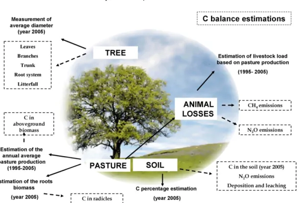
2.4.1. System description 219
To compare the carbon balance of the system, three main com- 220 ponents were considered:tree, soil and pasture(including animal 221 losses), as shown inFig. 1. The C stored in trees and soil was esti- 222 mated using data from 2005, while that of pasture was the average 223 of samples collected between 1995 and 2005. With the goal of 224 quantifying the potential GHG effect of the animals, we determined 225 an average annual pasture carrying capacity (PCC) that the system 226 could support based on actual annual pasture production in each 227
treatment (Steinfeld et al., 2006). 228
When calculating the potential GHG effect of livestock from 229 pasture production, the proportion of stable period/grazing period 230 must be taken into account according to the habitual pasture pro- 231 duction practices of the area (Mosquera and González, 1998), which 232 are determined by the seasonal interaction of precipitation and 233 temperature. Over the year, livestock is kept on pasture approx- 234 imately7months (April, May, June, July, 15 days in September, 235 October, November and 15 days in December) and stabled for 236 the remaining5months, during which the animals feed on grass 237 silage (approximately 150days year−1). The inclusion of the sta- 238 bling period in the global calculation of C is very important because 239 losses from the emission of N2O from livestock occur only during 240 this stabling period (IPCC, 1996). Of the various systems of manage- 241 ment proposed for the sheep that are raised for meat production 242 in Galicia (Zea-Salgueiro, 1992), those that are best adapted to the 243 conditions in our system are for sheep of the Galician breed of 35 kg 244
of live weight. 245
Silage area was taken into account to provide the same annual 246 basis C measurements for tree (which were growing up all the 247 year in the plots) and animals which were feed 210 days based 248
on grazing and 150 days on silage. 249
In order to calculate the annual stocking rate we sum up the 250 grazing area and the silage area. We deliver the number of animals 251 to be fed during the grazing period by taking into account the real 252 pasture production obtained under trees, afterwards, we calculate 253 the kilos of silage needed by these animals and, later, the number 254 of hectares needed to produce pasture to produce silage, and this 255
area is used to estimate annual stocking rate. 256
2.4.2. Estimation of pasture carrying capacity (PCC) 257
From the data of annual pasture production 258
(MgDM ha−1) and the forage necessary for sheep livestock 259 (1.74 kgDM sheep−1day−1) in a pasture (Flores et al., 1992), we 260 employedEq. (1)to estimate the pasture carrying capacity (PCC). 261
PCC (sheep ha−1)=P
C (1) 262
where PCC is the pasture carrying capacity; P is the annual pasture 263 production; and C forage requirements of grazing sheep for 210 264
days. 265
From the silage needs of 0.75 kgDM sheep−1day−1, as cited by 266 Flores et al. (1992), the known PCC, and the number of full days per 267 year that sheep are stabled (150 days), we determined the average 268
silage requirements usingEq. (2). 269
Total need of silage=0.75×PCC×150 (2) 270
UNCORRECTED PROOF
Fig. 1. Components of the system considered in order to evaluate the carbon balance in the study. The sampling period or year used to estimate the balance is shown between brackets.
Eq. (3).
278
Silage area= silage needed
silage production/ha (3)
279
After determining the pasture area needed for silage produc-280
tion to feed the flock that would be supported on our silvopastoral 281
system, we estimated the general system stocking rate (SRannual). 282
This metric captures the land area that is needed to maintain the 283
livestock annually and is calculated usingEq. (4).
284
SRannual=pasture areaPCC+silage area (4)
285
The pasture area was 1 ha because the calculation used to 286
determine the livestock sustained by pasture production in the 287
silvopastoral system was 1ha (Eq. (1)).
288
These figures were used to calculate the GHG emissions gener-289
ated by the livestock for each year. The global carbon balance was 290
determined using the average of those values. 291
2.4.3. Soil carbon estimation 292
2.4.3.1. Soil carbon storage. Once the actual percentage of edaphic 293
carbon was estimated in the laboratory, the content of carbon 294
in each of the treatments was calculated taking into account the 295
soil density (1.1Mg m−3) and the sample depth viaEq. (5).It was 296
found that soil density in the experiment did not significantly vary 297
between tree species or densities (Howlett, 2009). 298
C (Mg ha−1)=%C×soil volume×soil density
100 (5)
299
As most of the C was already on the soil before the plantation, 300
to estimate the C accumulated during those 11 years the difference 301
between the C in 2005 and that already in the system in 1995 was 302
calculated and divided by the years of the study(11).
303
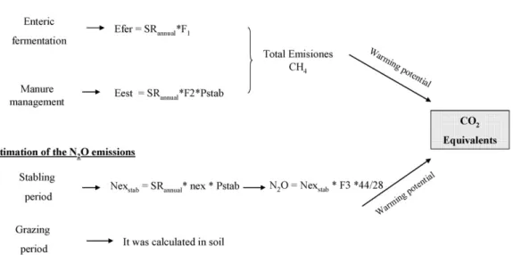
2.4.3.2. Soil carbon losses. Following the Guidelines of the IPCC 304
(1996), the direct and indirect N2O emissions were calculated for 305
the soil component in the different established systems (Fig. 2), 306 which were derived from the pasture carrying capacity of the sys- 307 tem previously calculated based on the actual pasture production. 308 To determine the equivalent CO2 amounts due to the N2O emis- 309 sions, the N2O emissions were multiplied by the warming potential 310 of N2O, which corresponds to a value of 310 based on theIPCC 311
report (1996). 312
(a) Directemissions of edaphic N2O 313
a.1Stabling period 314
The direct emissions of N2O resulting from the use of 315 manure as fertiliser were determined (Fig. 2). To do so, 316 we calculated the N excreted by the livestock (Nex) using 317 the previously calculated animal stocking rate and we then 318 determined the N in the manure used as fertiliser (Fe). Next, 319 an adjustment was made to the NH3 and NOxemissions 320 (Mosier et al., 1998; IPCC, 1996), excluding the manure pro- 321
duced during grazing. 322
a.2Grazing period 323
Estimates of N2O emissions during the grazing period 324 were calculated by using the N excreted by the live- 325 stock (Nex), using the pasture carrying capacity previously 326 calculated, and taking into account the emission factor 327 established by theIPCC (1996) for this type of land use 328
(Fig. 2). 329
(b) IndirectN2O emissions 330
UNCORRECTED PROOF
Fig. 2.Estimation of the N2O emissions (CO2equivalents) from the livestock for the soil, where NexT= total N excreted by the livestock (grazing + stabled); SRannual= stocking rate (sheep/ha); nex= nitrogen excreted from manure (20 kg N/animal unit/year (IPCC, 1996)); FE= N input from manure (kgN ha year−1);FracGRAZ= NexTfraction during grazing; FEGRAZ= emission factor (0.02 kgN2O-N/kg N);FracGASM= fraction of the total N excreted that is emitted as NOxor NH3(kgN/kg N = 0.2 kg NH3-N + NOx-N/kg N); FE1= emission factor (0.0125 kgN2O-N/kg of N input);NFER= N applied in the fertilisation treatments (NFER= 0); FracGASFS= fraction of the N applied in the fertiliser that is volatilized (when fertiliser is not applied then FracGASFS= 0); FracGASM= fraction of the total N excreted that isvolatilized (0.02 kg NH3-N + NOx/kgof N excreted by livestock); FE2= emission factor (0.01 kgN2O-N per kg NH3-N and NOx-N emitted); FracLIX= fraction of leached N (0.3 kgN/kg Nin manure); and FE3= emission factor (0.025 kg N2O-N per kg of N leaching and runoff). The values for the different factors in the formula are from theIPCC (1996)and correspond to the study area characteristics and the livestock considered (sheep).
by means of atmospheric deposition. This increases the pro-339
duction of N2O. Another portion is lost from the soil through 340
surface runoff and leaching, merging with surface and subter-341
ranean waters from which a proportion of this N is emitted as 342
N2O (Fig. 2). 343
2.4.4. Tree carbon estimation 344
Using the equation established byMontero et al. (2005)forP. 345
radiataandBetulaspp. (Table 1) and the data obtained from mea-346
suring the tree diameter at breast height, the aerial biomass of the 347
following components of the tree cover were determined: trunk, 348 thin and thick branches, leaves and roots(Eq. (6)). 349
Y=eSEE2/2×ea×db (6) 350
whereYis the biomass variable (biomass of trunk, biomass of the 351 branches with a diameter greater than 7 cm, biomass of branches 352 with a diameter within 2 cm and 7 cm, biomass of branches with a 353 diameter less than 2 cm, leaf and root biomass) anddis the diameter 354
at breast height (cm). 355
UNCORRECTED PROOF
Table 2
The pH and %C in soil (mean±standard error) at the time of establishment of the system and in the years 2000 and 2005 underPinus radiataandBetula albaat two densities
(2500 and 833 trees ha−1). Different letters indicate significant differences betweentreatments.ns: no significant difference.
Soil parameters Year Sig 2500 trees ha−1 833 trees ha−1
Pinusradiata Betula alba Pinus radiata Betula alba
pH Initial 6.8
2000 ns 5.4±0.12 5.4±0.15 5.1±0.00 5.8±0.00
2005 * 5.7±0.13b 5.9±0.14ab 6.3±0.32a 6.2±0.11a
%C Initial 4.6
2000 ** 5.84±0.45a 6.02±0.16a 4.39±0.54b 4.10±0.42b
2005 ns 5.30±0.99 6.22±0.67 4.75±0.35 5.21±0.15
MgC ha−1 Initial 126.50
2000 ** 160.74±12.45a 165.68±4.54a 120.68±14.91b 112.86±11.72b
2005 ns 145.80±27.21 171.00±18.34 130.69±9.68 143.41±4.30
*P< 0.07 for pH.
**P< 0.05 for C and MgC ha−1.
In Table 1, the values of SEE are shown, as well as the parameters 356
aandbthat were applied to calculate the biomass of each fraction. 357
Once this value was obtained, the C content for this biomass was 358
calculated by multiplying by an average value of 0.50 (Merino et 359
al., 2003; Montero et al., 2005). 360
2.4.5. Litterfall 361
The litterfall C content in the last year was obtained by mul-362
tiplying the litterfall biomass (MgDM ha−1) by a factor of 0.49 363
(Gómez-Rey and Calvo de Anta, 2002). 364
2.4.6. Pasture carbon estimation 365
From the data of pasture production (MgDM ha−1) obtained 366
for each of the treatments and in each year, the C content of 367
the herbaceous stratum was determined, distinguishing between 368
aboveground and belowground parts. 369
2.4.6.1. Aboveground. Above pasture C content could be divided 370
in two fractions: above and below 5 cm of aboveground pasture 371
height. C content determination of the 5 first cm of the pasture 372
aboveground fraction was not included in the model because this 373
is one of the sources of soil C, so it is already included in the system. 374
However, C content determination of aboveground pasture placed 375
above 5 cm from the soil was included because it will be mostly 376
storaged in the animal bodies, once excluding livestock GHG emis-377
sions, on an annual basis. The C content corresponding to the aerial 378
section of the herbaceous stratum was calculated on a yearly basis, 379
based upon the pasture production during the pasture season and 380
the need for silage. It was taken into account that when grass is 381
converted to silage, it suffers a 15% loss in weight (Mosquera and 382
González, 1998). Once the annual silage needed for the stabling 383 period was estimated with actual data obtained from the pasture 384 production that was attributed to the pasture season, we were able 385 to quantify the organic matter content in it(Eq. (7)).The percentage 386 of organic matter found in the pasture in Galicia is around 90.36% 387 (Flores et al., 1992), and the C content in a pasture will be 50% of 388
the organic matter (Montero et al., 2005). 389
OMpasture=(Mg DM pasture ha−1)×0.9036 (7) 390
2.4.6.2. Belowground.From the soil samples, and as in the pro- 391 cedure previously explained, we obtained a value of the ratio of 392
root/abovegroundbiomass in the pasture that was 32.37%. Then, 393 the root biomass was determined by applying this ratio to pasture 394 production (pasture production during pasture season + pasture 395 production during the stabling period). Once the root biomass was 396 determined, the C content was estimated to be 49.67% of that value 397
(Gordon et al., 2005). 398
2.4.7. Livestock 399
2.4.7.1. Estimation of livestock carbon losses. We estimated the CH4 400 and N2O emissions resulting from sheep livestock management, as 401 well as their equivalents in terms of CO2. The method used to esti- 402 mate this emission is described by theIPCC (1996). InFig. 3, the 403 equation and coefficients used in this study are shown, again, fol- 404 lowing the protocol of theIPCC (1996)and the guidelines indicated 405 for the regional estimation of carbon emissions established by the 406 government of the region in which the study was conducted (Xunta 407
de Galicia, 2004). 408
Table 3
Estimates of total N2O emission (direct and indirect) in Mgha−1from the soil during the 11 study years underPinus radiataandBetula albaat the2 stand densities (2500 and
833 trees ha−1).
Years 1995–2005 2500 trees ha−1 833 trees ha−1
Pinus radiata Betula alba Pinus radiata Betula alba
Direct
Stabling 5.44×10⁻³ 6.10×10⁻³ 5.85×10⁻³ 7.66×10⁻³
Pasturing 24.42×10⁻³ 27.38×10⁻³ 26.27×10⁻³ 34.41×10⁻³
Total 29.86×10⁻³ 33.48×10⁻³ 32.12×10⁻³ 42.07×10⁻³
Equiv CO2 9.25 10.38 9.96 13.04
Indirect
Deposition 0.43×10⁻³ 0.47×10⁻³ 0.46×10⁻³ 0.59×10⁻³
Leaching 15.54×10⁻³ 17.42×10⁻³ 16.72×10⁻³ 21.88×10⁻³
Total 15.97×10⁻³ 17.89×10⁻³ 17.18×10⁻³ 22.47×10⁻³
Equiv CO2 4.95 5.54 5.32 6.96
Total Equiv CO2 14.20 15.92 15.28 20.00
UNCORRECTED PROOF
Table 4
Tree measurements ofPinus radiataandBetula alba(mean±standard error) at two densities(2500 and 833 trees ha−1) and site index estimation at 20 years (Is). Different letters indicate significant differences between treatments (P< 0.001).
Year 2005 2500 trees ha−1 833 trees ha−1
Tree parameters Pinus radiata Betula alba Pinus radiata Betula alba
Basal diameter (cm) 15.0±0.49a 6.2±0.28b 16.8±0.87a 7.2±0.35b
(a) EstimatedCH4emissions 409
a.1Enteric fermentation estimates 410
To estimate enteric fermentation emissions, the pasture 411
carrying capacity (CG annual) and the average emissions 412
of CH4 per animal per year were taken into account. In 413
our case, with sheep, the value of the emission factor 414
is 5 kgCH4sheep−1year−1 (IPCC, 1996; Xunta de Galicia, 415
2004). 416
a.2Manure management emissions 417
To estimate manure management emissions, only the 5 418
months of stabling were taken into account. The animals 419
were stabled 41% of the days; thus, we multiply obtained 420
values by 0.41, which is the distribution percentage of the 421
use frequency in this type of manure management system. 422
Following the IPCC methodology, once the CH4emissions 423
from the livestock were obtained, the equivalent CO2was 424
determined taking into account the warming potential of 425
CH4, which has been established as 21 by theIPCC (1996). 426
(b) EstimatedN2O emissions from livestock 427
The N2O emissions result from both the stable and the pasture 428
periods (IPCC, 1996). 429
b.1 Stabling period 430
Emissions of N2O were calculated using the pasture car-431
rying capacity previously estimated for each treatment. 432
The quantity of excreted nitrogen (Nex) that resulted from 433
manure management was calculated by taking into account 434
the percentage of full days that livestock were stabled 435
throughout the year (41%). An emission factor was then 436
applied to this amount, which varies according to type of 437
livestock being considered, and is 20 kganimal−1year−1for 438
sheep (IPCC, 1996). Finally the CO2equivalents were deter-439
mined taking into account that the warming potential of 440
N2O is 310 (IPCC, 1996). 441
b.2 Pasturing period 442
This was calculated in the soil component (IPCC, 1996). 443
2.5. Statistical analyses 444
The pH, C in soil, tree diameter, tree height, and annual pasture 445
production variables were analysed by a factorial ANOVA, using 446
treatments and blocks as factors within each year. The significant 447
differences between means were determined using the LSD test 448
(SAS, 2001). 449
3. Results 450
3.1. Soil 451
During the course of the 11-year study, significant acidification 452 of the soils occurred. This is typical in the area due to high rainfall 453 and high levels of soil cation extraction from crops that bring acid- 454 ity in Galician soils. No significant differences were found between 455 treatments in relation to pH in the first5years of system produc- 456 tion (Table 2). However, 11 years later, there was a tendency for a 457 significant decrease in pH (P< 0.07), especially in the higher den- 458 sity plantations under pine species. On the other hand, the results 459 show a significant (P< 0.05) effect of treatments on the C con- 460 tent in the soil after5years of system development. A significant 461 increase in the soil C content (P <0.05) occurred in those systems 462 with the higher tree density (independent of species planted), an 463 effect which had disappeared at the 11-year mark (Table 2). From 464 the time that the system was established (126.50Mg C ha−1), inde- 465 pendent of the forest species used, an increase in the soil C content 466 was observed in 2005 over the level present at the time of planta- 467 tion establishment. This level of increase was greater in plots that 468 were established at higher tree densities (15% higher under pine 469
and 35% higher under birch). 470
3.1.1. Estimates of N2O emissions in the soil 471 For the 11 years of the study, the estimates of N2O emissions 472 for each of the different systems is shown inTable 3, as are the 473 equivalents in CO2emissions to the atmosphere. The results reflect 474 higher emission levels in those systems that were supporting a 475 higher pasture carrying capacity, i.e. those established under birch 476
cover, independent of the tree density. 477
3.2. Trees 478
The diameter reached byP.radiataduring the last year of the 479 study was significantly higher than that ofB.alba(Table 4). In regard 480 to diameter, the results show a similar tendency of tree density 481 on the development of each of the two forest species. Higher tree 482 densities favoured the lowest diameter, due to tree competition. 483
3.2.1. Tree carbon 484
In both forest species, the highest carbon accumulation occurred 485 in the aerial component (Table 5). In the conifer, high densities 486
Table 5
Total carbon in the tree biomass (Mg C ha−1) determined for the year 2005 by taking into account the average diameter obtained forPinus radiataandBetula albaat the two stand densities considered, where BF: trunk biomass; BR>7cm: biomass of branches greater than 7 cm; BR2–7cm: biomass of branches with diameters between 2–7cm; BR<2cm: biomass of branches less than 2 cm; BH: needles biomass (in pine) or leaf biomass (in birch); Br: root biomass.
Total carbon Caerial biomass (MgC ha−1) Root biomass (MgC ha−1)
Density d(cm) BF BR>7cm BR2–7cm BR<2cm BH Total aerial Br Total
Pinus radiata 2500 15.03 62.95 0.71 7.43 5.08 2.54 78.71 26.89 105.61
833 16.78 27.88 0.36 3.13 2.06 1.06 34.49 11.35 45.84
Betula alba 2500 6.25 10.07 0.00 2.95 1.76 0.85 15.63 4.67 20.30
UNCORRECTED PROOF
Table 6
Amount of carbon content in the aboveground part of the pasture (pasture + silage) in the establishedPinus radiatasystems for each year of the study (1995–2005),where PCC = pasture carrying capacity; SRannual= system stocking rate. Grazing and stabling period lasted 210 and 150 days per year. Food sheep requirements per day were 1.74kg
of pasture and 0.75 kg of silage. Silage production was 7096 kg DM silo per year. Letters in the pasture production column indicates significant differences between treatments within the same year.
Year Pasturingperiod Stabling period
Pasture production PCC Silage requirements Silage area SRannual Total herbaceous Average C
kg DM ha−1 sheep ha−1 kg DM silage ha−1 year−1 ha sheep ha−1 (Pasture + silage) (kg DMha−1) Mg C ha−1 (Mg C ha−1 year−1)
2500 trees ha−1Pinus radiata
1995 3450 9 1013 0.14 8 4463 2.02
1.46
1996 3770 10 1125 0.16 9 4895 2.21
1997 1280b 3 338 0.05 3 1618 0.73
1998 3230 9 1013 0.14 8 4243 1.92
1999 3230 9 1013 0.14 8 4243 1.92
2000 2720b 7 788 0.11 6 3508 1.58
2001 5720ab 16 1800 0.25 13 7520 3.40
2002 530b 1 113 0.02 1 643 0.29
2003 1070 3 338 0.05 3 1408 0.64
2004 1290 4 450 0.06 4 1740 0.79
2005 960b 3 338 0.05 3 1298 0.59
833 trees ha−1Pinus radiata
1995 5200 14 1575 0.22 11 6775 3.06
1.63
1996 3300 9 1013 0.14 8 4313 1.95
1997 3590ab 7 788 0.11 6 4378 1.53
1998 1640 4 450 0.06 4 2090 0.94
1999 1850 5 563 0.08 5 2413 1.09
2000 3280b 9 1013 0.14 8 4293 1.94
2001 5590ab 15 1688 0.24 12 7278 3.29
2002 2390a 6 675 0.10 5 3065 1.38
2003 2220 6 675 0.10 5 2895 1.31
2004 1640 4 450 0.06 4 2090 0.95
2005 970b 3 338 0.05 3 1308 0.59
2500 trees ha−1Betula alba
1995 3430 9 1013 0.14 8 4443 2.01
1.67
1996 2860 8 900 0.13 7 3760 1.70
1997 2010ab 5 563 0.08 5 2573 1.16
1998 3270 9 1013 0.14 8 4283 1.94
1999 2700 7 788 0.11 6 3488 1.57
2000 2050b 6 675 0.10 5 2725 1.23
2001 2910b 8 900 0.13 7 3810 1.72
2002 1310ab 4 450 0.06 4 1760 0.79
2003 2650 7 788 0.11 6 3438 1.55
2004 4060 11 1238 0.17 9 5298 2.39
2005 4110a 11 1238 0.17 9 5298 2.39
833 trees ha−1Betula alba
1995 4870 13 1463 0.21 11 6333 2.86
1.63
1996 3700 10 1125 0.16 9 4825 2.18
1997 3870a 11 1238 0.17 9 5108 2.31
1998 3090 8 900 0.13 7 3990 1.80
1999 3110 8 900 0.13 7 4010 1.81
2000 5330a 15 1688 0.24 12 7018 3.17
2001 7680a 21 2363 0.33 16 10043 4.54
2002 2020a 6 675 0.10 5 2695 1.22
2003 2750 7 788 0.11 6 3538 1.60
2004 1990 5 563 0.08 5 2553 1.15
2005 2440ab 7 788 0.11 6 3228 1.46
increase C fixation per unit surface area around 43% with respect 487
to the lower density plantations, and in the deciduous species, this 488
increase was 51%. The average C accumulation during the11-year
489
period in theP.radiatastand was 9.86Mg C ha−1year−1at a density 490
of2500 trees ha−1and 4.35 Mg C ha−1year−1with 833 stems ha−1. 491
In theB.albastand, it was 1.84 and 0.94Mg C ha−1year−1 for the 492 densities of2500 and 833 trees ha−1, respectively. If we compare 493 the effect of density on the two forest species, we see that at triple 494 the density, the carbon content in the aerial component of the 495 timber doubled; this increase was slightly higher in the pine. 496
Table 7
Amount of carbon content (Mgha−1) in the roots of the herbaceous component of the systems evaluated.
Year 2005 2500 trees ha−1 833 trees ha−1
Pinusradiata Betula alba Pinus radiata Betula alba
Pasture + silage (kg DMha−1) 1298 5298 1308 3228
Root (kg DM ha−1) 420 1715 423 1045
UNCORRECTED PROOF
Table 8
Estimates of the total emissions (Mgha−1) of methane (ECH
4) and oxides of nitrogen (EN2O) due to the manure management of livestock during the period between1995 and
2005, whereEfer: CH4emissions from enteric fermentation;Eest: CH4emissions from manure management; Nex: total N excreted by livestock during the 11 years of the study, andEquiv CO2: CO2equivalents (Mgha−1).
Years 1995–2005 2500 trees ha−1 833 trees ha−1
Pinus radiata Betula alba Pinus radiata Betula alba
ECH4
Efer 0.330 0.370 0.355 0.465
Eest 6.0×10⁻³ 6.7×10⁻³ 6.4×10⁻³ 8.4×10⁻³
Total 0.336 0.377 0.361 0.473
Equiv CO2(Mgha−1) 7.06 7.91 7.58 9.93
EN2O
Nex 0.541 0.607 0.582 0.762
N2O 17×10−3 19×10−3 18×10−3 24×10−3
Equiv CO2(Mg ha−1) 5.3 5.9 5.6 7.4
Total Equiv CO2(Mgha−1) 12.36 13.81 13.19 17.33
3.3. Litterfall 497
Litterfall content in the pine plots in 2005 was 6.25Mg ha−1 498
at a density of2500 trees ha−1and 4.26 Mg ha−1at 833 trees ha−1. 499
This resulted in an average C content of 3.06Mg C ha−1year−1 500
and 2.09 Mg C ha−1year−1 at the higher and lower densities, 501
respectively. Generally, as occurs with the aboveground biomass, 502
the capacity for needle accumulation in the soil incrementally 503
increases with stand density, which is attributed to the earlier 504
canopy closure in the higher density stands. Of the total fixed car-505
bon in the tree stratum, the percentage of carbon accumulation 506
accounted for by the fallen needles was 2.9% at a tree density of 507
2500 trees ha−1 and 4.5% at 833 trees ha−1. This indicates that, at 508
triple the density, the greater litterfall increased carbon storage by 509
approximately 55%. Therefore, as was found with carbon storage in 510
the living tree component, this C also doubled. 511
3.4. Pasture 512
3.4.1. Aboveground 513
The results show a significant effect of the applied treat-514
ments on pasture production in the years 1997, 2000, 2001, 515
2002, and 2005 (Table 6). The average production during the 516
course of the study at 2500 and 833 trees ha−1, respectively, 517
was 2.5 and 2.8Mg ha−1year−1 in the pine systems and 3.8 and 518
3.7 mgha−1year−1under birch. Furthermore, during the trial, the Q2
519
increasing light interception significantly reduced pasture produc-520
tion in the pine stands, whereas under the birch, pasture production 521
was more dependent from other climate parameters. On the other 522
hand, in 2001, as a result of the low pruning in the systems and 523
an unusually rainy summer, an increase in pasture production was 524
observed, independent of the tree density or forest species. 525
Table 6 shows the C content measured in the aboveground 526
herbaceous layer (pasture during grazing season + pasture for 527
silage) throughout 11 years (1995–2005).The amount of C accumu-528
lated during the 11 years of system growth resulted in an increase 529
of 1.46Mg C ha−1and 1.63 Mg C ha−1under pine cover at2500 and 530
833 trees ha−1, respectively. In the systems established under birch, 531
the estimates were 1.67Mg C ha−1and 2.19 Mg C ha−1for the lower 532
and higher densities, respectively. 533
3.4.2. Belowground 534
In 2005, the estimated amount of C in the fine roots was 535
0.21Mg C ha−1 under pine for both of the two plantation densi-536
ties. Under birch, we obtained estimates of 0.85Mg C ha−1 and 537
0.52 Mg C ha−1at 2500 and 833 trees ha−1, respectively (Table 7). 538
3.5. Estimation oflivestockcarbon losses 539
The estimate of the total CH4and N2O emissions from the live- 540 stock, as well as the equivalents in CO2, are reported inTable 8. 541 The emissions of CH4 and N2O on the part of the livestock were 542 greater in those systems that combined lower plantation densities 543 with deciduous tree coverage (although they were always less than 544 10Mg CO2ha−1) because these systems supported higher animal 545
stocking rates. 546
3.6. Balance of carbon 547
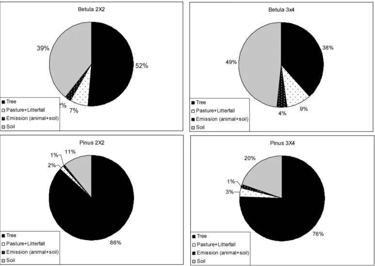
The final balance of the carbon cycle, calculated for the differ- 548 ent systems studied, is shown inFigs. 4 and 5, and the relative 549 proportion of each component (pasture, litterfall, animals, trees, 550 and soil) is given inFig. 6. If we compare the capacity for car- 551 bon sequestration at the end of the experiment (MgC ha−1year−1) 552 among the different components of the system, the tree shows the 553 highest level of C fixation, followed by soil, and finally, by pasture 554 (tree > soil > pasture). The exception occurs in the systems planted 555 with birch at low density, in which the C stored in the soil compo- 556 nent is higher than that of the tree (soil > tree > pasture) due to the 557
lower rate of tree growth. 558
Our estimates show a tendency, though not significant, of 559 a greater capacity to fix carbon in the systems with higher 560 plantation density (8.19Mg C ha−1year−1 in 2500 trees ha−1 and 561
6.75 Mg C ha−1year−1in 833 trees ha−1), especially in the case of 562 the pine. On the other hand, if we compare the two forest species, 563 the estimates reflect a clear tendency (P <0.05) of a greater car- 564 bon sequestration capacity in the silvopastoral systems planted 565 with pine (10.95 and 3.99Mg C ha−1year−1 forPinusand Betula, 566
respectively). 567
Fig. 6shows the relative proportion of the various system com- 568 ponents in relation to their carbon sequestration at the end of the 569 experiment. The relative contribution of each component to the 570 carbon balance at the end of the experiment changes within each 571 system. In the case of the birch, the contribution of carbon in the soil 572 to the total carbon in the system is greater than in the pine (P= 0.05; 573 44% compared to 15%). This becomes especially pronounced at the 574 lower stand density. In contrast, the relative contribution of the 575 tree component to the total system, excluding litterfall, is higher in 576 the pine than in the birch (81% of the total for the pine compared to 577 45% of the birch;P= 0.05). In all cases, livestock emissions remained 578 counterbalanced by the carbon accumulated in the pasture and in 579
the litterfall. 580
UNCORRECTED PROOF
Fig.4.
Carbon
balance
(Mg
Ch
a
−
1year
−
1)
for
those
systems
established
under
Pinus
radiata
D.
Don
at
plantation
densities
of
2500
and
833
trees
ha
−
UNCORRECTED PROOF
Fig.
5.
Carbon
balance
(Mg
Ch
a
−
1year
−
1)
for
those
systems
established
under
Betula
alba
L.
at
plantation
densities
of
2500
and
833
trees
ha
−
UNCORRECTED PROOF
Fig. 6.Relative contribution to C storage in tree, pasture + tree litterfall, animal and soil components in each system expressed after 11 years of experiment.
storage differ markedly. The results show a far superior contri-584
bution of carbon from the trees from the more densely planted 585
pines compared to all other treatments. Within the pine plan-586
tations, the stand density changes the percentage of C storage 587
capacity of all of the components, as occurs in the birch system 588
when the edaphic component is excluded. However, this contribu-589
tion does not vary between forest species at the same plantation 590
densities. 591
4. Discussion
592
Carbon sequestration in both soil and aboveground biomass 593
is one of the most important benefits of the afforestation of 594
agricultural lands (Maia et al., 2007; Nair et al., 2007). Carbon 595
sequestration in woody biomass is promoted as a practice to off-596
set increasing atmospheric CO2concentrations (Sauer et al., 2007). 597 However, extensive analyses of forest productivity for various 598 forest types and management practices have been primarily com- 599 pleted for tree aboveground biomass, usually without assessment 600
of the understory. 601
The C content has been found to be higher in conifer forests 602 due to the higher growth rate of this species compared to that of 603 birch (Bunker et al., 2005; Kirby and Potvin, 2007).P.radiatahas 604 a greater C sequestration in the biomass compared to birch at the 605 same plantation densities, by 21% at2500 trees ha−1and by 9.5% at 606
833trees ha−1, after 11 years. 607
The rate of carbon sequestration of the conifer plantations in 608 our study was less than that normally expected in silvopastoral 609 systems, like those of New Zealand, due not only to the lower tree 610 density (Chang and Mead,2003), but also to the higher site index 611
Table 9
Relative carbon allocation (estimated as MgC ha−1) to the storage pools of the different agroforestry systems. Different letters indicate significant differences between treatments in each of the components (P< 0.05).
% Carbon allocation
Pinus radiata Betula alba
2500 trees ha−1 833 trees ha−1 2500 trees ha−1 833 trees ha−1
Tree 41.58a 10.04bc 26.29ab 5.04c
Pasture + litterfall 7.92c 12.65ab 10.95bc 16.30a
UNCORRECTED PROOF
(better climatic conditions and soil fertility) and age of the stands 612
analysed in New Zealand (Lavery, 1986). In regard to the birch, 613
the carbon sequestration capacity we obtained is similar to that 614
found in the Nordic countries of Europe (Karlsson et al., 1998). 615
In our case, a decrease in forest productivity occurs due to sum-616
mer drought, whereas the Nordic countries experience a similar 617
decrease in productivity during the winter cold. 618
The sequestration of C when a tree component is present is 619
also impacted by the density of the established plantation. In this 620
study, the difference in C sequestration capacity increased by 28% 621
and 18% in pine and birch, respectively, at the higher density. 622
When establishing a silvopastoral or forest system in an agricul-623
tural zone with no competition between trees, there is a direct 624
relationship between the system’s capacity for C sequestration and 625
the plantation density. However, in the future, this capacity could 626
be limited as the competition among trees increases and limits 627
growth. 628
During the first years, pasture production in the systems was 629
similar for both plantation densities, resulting in no effect of tree 630
coverage on production. As a result of tree growth and, conse-631
quently, tree canopy, the microclimate conditions of the systems 632
change and influence pasture production. Differences in planta-633
tion densities and among distinct ecological patterns of pine and 634
birch are also known to influence pasture production (Sibbald et 635
al., 1991; Silva-Pando et al., 2002). Likewise, as the system devel-636
ops, the C sequestration capacity of the pasture diminishes, as the 637
biomass production is reduced when lower amounts of light are 638
able to reach the herbaceous layer. In our case, the amounts of 639
C sequestration recorded aboveground on pastures show that sil-640
vopastoral systems in which the parameters of tree cover (growth 641
rate, crown shape, deciduous leaves, needles) allow the pasture 642
to expand and maintain a high production rate over time have a 643
higher accumulation rate of carbon in this component. When com-644
paring pasture production under pine versus under birch, we find 645
that production under birch is higher due to the more light that 646
reaches the understory, the slower growth rate of the tree, and 647
the canopy shape. Therefore, these factors contribute to the higher 648
capacity for carbonabsorbedby the pasture component under birch 649
cover. 650
The reduction of C sequestration capacity in the pasture can 651
be compensated for by the C accumulation in tree litter on the 652
forest floor in the systems with pines planted at high densities 653
(Vesterdal et al., 2002). This result is consistent with our find-654
ings in those systems established under higher density stands 655
(2500 trees ha−1), where the decrease in pasture production that 656
occurred under pine cover, as well as the consequently lower C 657
content that accumulated, was partially compensated for by the 658
carbon accumulation in the litter layer of these systems. Ultimately, 659
there was a 25% reduction in C accumulation when compared to 660
the levels accumulated in pastures growing under birch (1.9 and 661
2.5Mg C ha−1year−1under pine and birch cover, respectively). The 662
results were nearly identical in the lower tree density systems 663
(833trees ha−1) in that the accumulation of carbon in the litter 664
under pine (2.03Mg C ha−1year−1) was also 25% lower than that 665
in the pasture component under birch (2.71Mg C ha−1year−1). The 666
presence of herbaceous pasture or litterfall in our system will have 667
varying effects on the rate of the carbon incorporation of these 668
residues into the soil. In forest systems, litterfall on the soil surface 669
is the primary organic input, but in many cropping and grassland 670
systems, the primary organic input is the decomposition of the 671
roots and senescent pasture material (Gale and Cambardella, 2000). 672
On the other hand, the higher pasture production occurring in 673
the birch systems could, in turn, provoke a larger production of GHG 674
from the livestock, and thereby, a greater pasture carrying capacity 675
than could otherwise be sustained. The C emitted by the animals 676
translates, in all of the treatments, into 40% of the carbon stored in 677 the herbaceous component. The reduced pasture carrying capacity 678 that could be sustained by the silvopastoral systems considered in 679 this study, in comparison with exclusively pastoral systems within 680 this zone (Mosquera and González, 1998), result in less estimated 681 emissions that are also compensated by the sequestration of C in 682 the other components of the system (tree and soil). This implies 683 that the C emissions on the part of the ruminants can be related 684 to the use of animal stocking rates that are neither adjusted to the 685 production capacity of the system, nor related to the elevated pas- 686 ture carrying capacity and animal production that occurs in systems 687 that are not based on pasture production. In other words, it is based 688 on stabling of the animals or intensive farming. 689 Soil is the final destination for the majority of carbon fixed 690 by photosynthesis in the Earth’s ecosystems, and can be a major 691 sink of atmospheric CO2(Lal, 2004). Furthermore, this soil carbon, 692 in many forest systems, can remain stored for hundreds of years 693 (Bouwman, 1990). Forest management, including a change in tree 694 species and density, has been accepted as a measure of mitigation 695 of atmospheric CO2in national greenhouse gas budgets (Vesterdal 696 et al., 2008). However, quantitative estimates of tree species effects 697 on soil C pools are still scarce (Vesterdal et al., 2008). Soil car- 698 bon sequestration in a silvopastoral system depends, among other 699 things, on(i)organic matter inputs from pasture and tree residues, 700
(ii)the litterfall quality and quantity from the tree and pasture, and 701
(iii)the mineralisation rate, which depends on soil chemical char- 702 acteristics, like the pH, and environmental factors, like temperature 703 and humidity, which are also affected by tree species. In our study, 704 establishing a forest on abandoned agricultural land with a nearly 705 neutral pH caused an increase in acidity in the soil 11 years after 706 planting (Mosquera-Losada et al., 2006). Low soil pH may inhibit lit- 707 ter decomposition and the incorporation of litter C into soil organic 708 carbon (Sauer et al., 2007). Thus, in our case, few differences were 709 detected between pine and birch in relation to soil carbon accumu- 710 lation after 11 years, but, both have higher final C storage than in the 711 initial conditions. However, SOC sequestration in deeper soil layers 712 could be more important underP. radiatathanB.albadue to bet- 713 ter coarse root development (Fontaine et al.,2007;Li et al., 2007). 714 Studies carried out in the same experiment in 2007 (Howlett, 2009) 715 revealed that around 25% of organic carbon were placed between 716 25 and 1 m of depth, which means that most of the SOC was in the 717 first 25 cm as foundJiménez et al. (2008)in dry tropical forests. No 718 significant differences on total SOM concentration between den- 719 sities or tree species were found in the 25–50, 50–75 and 75–100 720 soil depth layers (Howlett, 2009). Moreover, the proportion of fine 721 roots, main source of SOM in deeper soil layers were also very low 722
in this experiment (Howlett, 2009). 723
UNCORRECTED PROOF
viously managed for crop or forage production has the potential 742
to significantly alter soil properties (Paul et al., 2002). The distinct 743
rates of organic matter production that depend on the tree type 744
and density found in our case eventually influence soil organic car-745
bon (Lugo and Brown, 1993; Guo and Gifford, 2002). Each species 746
(broadleaf and conifer) has a different carbon allocation strategy 747
that results in a different pattern, rate, quality, and quantity of 748
organic carbon input to the soil (Lugo and Brown, 1993; Guo and 749
Gifford, 2002). In our case, systems established under birch tended 750
to demonstrate a greater rate of C accumulation and storage in the 751
soil compared to those established under pine at the higher den-752
sities, despite the notably inferior rate of forest production (Lal et 753
al., 1995). 754
Large differences were found in the annual system balance of 755
carbon sequestration in the studied systems being more important 756
for pines. There were also appreciable differences in the alloca-757
tion of carbon to the different components of the systems studied. 758
In any case, systems underdensely plantedconifers had a major 759
proportion of carbon in the tree, compared to broadleaf stand and 760
to lower density pine stand. Since differences in the global bal-761
ance of carbon were found, it is clear that carbon stored in this 762
system would remain shorter time in this area because, once the 763
timber is harvested, potentially 50% of the system’s carbon could 764
be extracted from this type of forestland. This would not occur in 765
the case oflow-densitytreatments in which the majority of car-766
bon is stored in the soil and is, consequently, more enduring. It 767
is important to note that this differential division of carbon will 768
cause differences in forest management decisions regarding car-769
bon balance. After a thinning, the reduction of stored carbon in a 770
high-density plantation of conifer would be directly affected by the 771
removal of those trees, and in the case of thelow-density planta-772
tion, by the effect that the removal of trees would have on the soil. 773
The highest production of pasture occurred under deciduous trees 774
at low density, which also had the highest accumulation of carbon 775
in the soil due to the fast integration of the leaf into the soil. This dif-776
ference was compensated for, however, by a higher accumulation 777
of carbon in the tree in the case of the higher density pine planta-778
tions as was described byPalma et al. (2006)which indicates that 779
the main difference in sequestration between an arable system and 780
an agroforestry system lies in the carbon immobilized in the tree 781
biomass. 782
In our region, agroforestry systems planted under deciduous 783
trees atlow-densityresult in the highest compatibility with ani-784
mal production, since the deciduous trees allow for higher pasture 785
production and, therefore, a higher annual profitability for the 786
landowner. Even though, global levels of carbon sequestration in 787
birch were lower than in pines, the storage of C was more linked 788
to the soil in the deciduouslow-densitytree plantations, which 789
results in a more enduring storage capacity. This has a notable 790
socio-economic impact if environmental, as opposed to low qual-791
ity wood production issues, are taken into account for afforestation 792
policies. 793
In conclusion,at the end of 11 years, the establishment of an 794
agroforestry system resulted in an increase in carbon sequestra-795
tion capacity. We found that tree density first and forest species 796
secondly had significant impacts on the differential capacity to 797
sequester carbon within the system. The largest stock of carbon 798
was found in the trees in all cases, with the exception of the birch 799
systems at the lower density. This resulted in a significant differ-800
ence in the amount of GHG emissions by the livestock if the pasture 801
carrying capacity was adjusted to pasture production, or in other 802
words, with extensive systems. 803
On the other hand, reforestation withlow-densitybirch rather 804
than pine would generate higher edaphic C sequestration rates, 805
while still allowing for reasonable pasture production.
Uncited reference Q3 806
Stephan et al. (2000). 807
Acknowledgements 808
This paper has been completed thanks to the financial assistance 809 of the Spanish Ministry and Xunta de Galicia. The authors would like 810 to thank Teresa López Pi ˜neiro, José Javier Santiago Freijanes, Div- 811 ina Vázquez Varela, Pablo Fernández Paradela and Mónica García 812 Fernández for their collaboration in the realisation of this study. 813
References 814
Bouwman, A.F., 1990. Exchange of greenhouse gases between terrestrial ecosystems 815 and the atmosphere. In: Bouwman, A.F. (Ed.), Soils and theGreen House Effect. 816
Wiley, Chischester, pp. 61–127. 817
Bunker, D.E., DeClerk, F., Bradford, J.C., Colwell, R.K., Perfecto, I., Phillips, O.L., 818 Sankaran, M., Naeem, S., 2005. Species loss and above-ground carbon storage 819 in a tropical forest. Science 310 (5750), 1029–1031. 820 Calvo de Anta, R., Macías, F., Riveiro Cruz, A., 1992. Aptitud agronómica de la 821 provincia de La Coru ˜na (cultivos, pino, roble, eucalipto y casta ˜no). University 822 of Santiago de Compostela, Spain (in Spanish). 823 Chang, S.X., Mead, D.J., 2003. Growth of radiate pine (Pinus radiataD. Don) as 824 influenced by understory species in a silvopastoral system in New Zealand. 825
Agroforest. Syst. 59, 43–51. 826
Dixon, R.K., 1995. Agroforestry systems: sources or sinks of greenhouse gases? Agro- 827
forest. Syst. 31, 99–116. 828
EC, 2005. Communication on the implementation of the EU Forestry Strat- 829
egy. In: Commission Staff Working Document (accessed 1.06.09.) 830 http://ec.europa.eu/agriculture/publi/reports/forestry/workdoc en.pdf. 831 EEA (European Environment Agency), 2003. Europe’s environment: the Third 832
Assessment. EEA, Copenhagen, http://reports.eea.europa.eu/environmental 833
assessment report 2003 10/en/kiev chapt 00.pdf. 834
EU, 1992. COUNCIL REGULATION (EEC) No 2080/92 of 30 June 1992 Institut- 835
ing a Community aidScheme for Forestry Measures in Agriculture (accessed 836
15.05.09.) http://www.legaltext.ee/text/en/T30207.htm. 837
EU, 2005. Council regulation (EC) n◦ 1698/2005 of Septembre 2005 on Sup- 838
port for Rural Development by the European Agricultural Fund for Rural 839 Development (EAFRD) (accessed 15.05.09.) http://eurlex.europa.eu/LexUriServ/ 840 LexUriServ.do?uri=OJ:L:2005:277:0001:0040:EN:PDF. 841 FAO-ISRIC-ISSS,1998. World Referente Base for Soil Resources. World Soil Resources 842
Reports 84. FAO, Rome. 843
Fernández-Nú ˜nez, E., Rigueiro-Rodríguez, A., Mosquera-Losada, M.R., 2007. Eco- 844 nomic valuation of different land use alternatives: forest, grassland and 845 silvopastoral systems. Grass. Sci.Eur. 12, 508–511. 846 Fontaine, F., Barot, S., Barré, P., Bdioui, N., Mary, B., Rumpel, C., 2007. Stability of 847 organic carbon in deep soil layers controlled by fresh carbon supply. Nature 848
450, 277–280. 849
Flores Clavete, G., Gónzalez Arráez, A., Díaz Nú ˜nez, M.,1992. Producción ovina sobre 850
praderas de zona costera de Galicia: efecto del sistema de pastoreo (rotacional 851 y continuo) y de tres niveles de intensidad de pastoreo sobre la producción de 852 pasto y producción animal. Xunta de Galicia, Spain (in Spanish). 853 Gale, W.J., Cambardella, C.A., 2000. Carbon dynamics of surface residue- and root- 854 derived organic matter under simulated no-till. Soil Sci. Soc. Am. J. 64, 190–195. 855 Gómez-Rey, M.X., Calvo de Anta, R., 2002. Datos para el desarrollo de una red 856 integrada de seguimiento de la calidad de suelos en Galicia (N.O. de Espa ˜na): Bal- 857 ances geoquímicas en suelos forestales (Pinus radiata). 1. Aportes de elementos 858 por deposición atmosférica y hojarasca. Edafología 9 (2), 81–196. 859 Gordon, A.M., Naresh, R.P.F., Thevathasan, V., 2005. How much carbon can be stored 860 in Canadian agroecosystems using a silvopastoral approach? In: Mosquera- 861 Losada, M.R., McAdam, J., Rigueiro-Rodríguez, A. (Eds.), Silvopastoralism and 862
Land Sustainable Management. CABInternational, Wallinford, pp. 210–219. 863 Guitián-Ojea, F., Carballás-Fernández, T., 1976. Técnicas de análisis de suelos. Pico 864
Sacro, Spain (in Spanish). 865
Guo, L.B., Cowie, A.L., Montagu, K.D., Gifford, R.M., 2007. Carbon and nitrogen stocks 866 in a native pasture and an adjacent 16-year-oldPinus radiataD. Don plantation 867 in Australia.Agric. Ecosyst.Environ. 124 (3–4), 205–218. 868 Guo, L.B., Gifford, R.M., 2002. Soil carbon stocks and land use change: a meta analysis. 869
Glob. Change Biol. 8 (2), 345–360. 870
Howlett, D., 2009. Environmental amelioration potential of silvopastoral agro- 871 forestry systems of Spain: soil carbon sequestration and phosphorus retention. 872 PhD Thesis. University ofFlorida, USA, p.178. 873 IPCC (IntergovernmentalPanel on Climate Change), 1996. Reporting Instructions 874 Guidelines for National Greenhouse Gas Inventory,vol. 2. Intergovernmental 875
Panel on Climate Change, http://www.ipcc.ch/about/index.htm. 876 Jiménez, J.J., Lal, R., Leblanc, H.A., Russo, R.O., Raut, Y., 2008. The soil C pool in different 877 agroecosystems derived from the dry tropical forest ofGuanacaste, Costa Rica. 878