Attribute-value inference using deep neural networks

(1)

University Institute of Lisbon

Department of Information Science and Technology

Attribute-Value Inference using

Deep Neural Networks

Kevin Almeida Ramos

A Dissertation presented in partial fulfillment of the Requirements

for the Degree of

Master in Computer Science and Business Management

Supervisor

Ricardo Daniel Santos Faro Marques Ribeiro, Assistant Professor,

Ph.D.

ISCTE-IUL

Supervisor

Sancho Moura Oliveira, Assistant Professor, Ph.D.

ISCTE-IUL

(2)

(3)

"We are prisoners of the present, in perpetual transition from an inaccessible past to an unknowable future."

(4)

(5)

Abstract

The population’s consumption patterns have changed over the last few years and e-commerce has been one of the main drivers. The consumer became very demand-ing and very knowledgeable about the product and the websites were adaptdemand-ing, providing more information and improving the filtering system by adding detailed descriptions of the products and their characteristics. Extracting different charac-teristics from thousands of products is a task with a very high cost. In this work, we created three datasets that were later used by our model with three layers, CNN-BiLSTM-CRF, to infer values of attributes of previously unknown products through the description of products. It inferred with 64% of macro average of f1-score, not being related to the state of the art due to the different context of the tests.

Keywords: Named Entity Recognition, Information Extraction, Neural Se-quence Labeling

(6)

(7)

Resumo

Os padrões de consumo da população alteraram-se nos últimos anos e o e-commerce foi um dos grandes responsáveis. O consumidor tornou-se muito exigente e bas-tante conhecedor do produto e os websites foram-se adaptando, disponibilizando mais informação e melhorando o sistema de filtragem, adicionando descrições de-talhadas dos produtos e as suas características. Extrair diferentes características de milhares de produtos é uma tarefa com um custo bastante elevado. Neste trabalho, criamos três conjuntos de dados que posteriormente foram usados pelo nosso modelo com três camadas, CNN-BiLSTM-CRF, para inferir valores de atrib-utos de prodatrib-utos anteriormente desconhecidos através da descrição dos prodatrib-utos. Inferiu com 64% de macro média de f1-score, não sendo relacionável com o estado de arte devido ao contexto dos testes serem distinto.

Palavras-chave: Reconhecimento do nome da entidade, Extração de Infor-mação, Etiquetagem Sequencial Neuronal

(8)

(9)

Acknowledgements

To my supervisors, Professor Ricardo Ribeiro and Professor Sancho Oliveira I would like to thank them for sharing their visions, knowledge and mentoring.

To the Instituto de Telecomunicações for the supply of all the necessary ma-terial.

To my friends and colleagues who helped me on this long journey, thank you for the good times.

To the family, and especially to my parents for all their tireless support, always supporting me to continue my academic education and to follow my dreams.

(10)

(11)

List of Tables

1.1 Mapping of chapters associated with the DSR methodology . . . 5

2.1 Example of POS Tags from Penn Treebank Project . . . 10

2.2 BIO Chunk Tag scheme. . . 11

3.1 A summary of public e-Commerce datasets. . . 24

3.2 A summary of neural sequence labeling models. . . 28

4.1 Custom Entity Tag with BIO tag scheme using Figure 4.7 as example 35 5.1 Datasets Structures . . . 43

5.2 Meaning of metrics . . . 45

5.3 Hyperparameters used in the model . . . 46

5.4 F1-score comparison of the different datasets. . . 47

5.5 Jewels dataset deduced from Fashion dataset. . . 48

5.6 HomeDecor dataset deduced from Fashion+ dataset. . . 48

5.7 Comparison between the gold label and the prediction - Jewels dataset deduced from Fashion. . . 49

5.8 Comparison between the gold label and the prediction - HomeDecor dataset deduced from Fashion+ . . . 50

(14)

(15)

List of Figures

1.1 Evolution and expectation of the number of e-Commerce users . . . 2

1.2 Design Science Research Process Model . . . 4

1.3 DSR Knowledge Contribution Framework . . . 5

2.1 Example of a filtering system of the Charme 24 . . . 8

2.2 Pipeline Architecture for an Information Extraction System . . . . 9

2.3 Example of tagger context works using n-gram . . . 10

2.4 Example of a "one-hot" vector structure . . . 13

2.5 Example of a word embedding structure with the floating-point val-ues represented . . . 13

2.6 CBOW and Skip-gram models of Word2Vec. . . 14

2.7 BERT model architecture. . . 15

2.8 Simple feed-forward neural network . . . 16

2.9 Standard Recurrent Neural Network single tanh layer . . . 16

2.10 Long Short-Term Memory architecture . . . 17

2.11 Example of CNN architecture. . . 18

2.12 Example of sparse connectivity. . . 19

2.13 Example of max pooling layer effect. . . 20

2.14 Linear chain-structured CRFs. . . 21

4.1 Pipeline of our approach. . . 29

4.2 Example of a product description from Jewels dataset. . . 31

4.3 Example of a product description from Fashion dataset. . . 32

4.4 Example of a product description from HomeDecor dataset. . . 32

4.5 Example of a product description extracted from product page . . . 33

4.6 Example of a attribute-values extracted from the product page . . . 34

4.7 Example of product description with custom entities tags. . . 35

4.8 Architecture of our neural network. . . 36

4.9 Character-level information encode into Convolutional Neural Net-work. . . 37

4.10 Architecture of Bidirectional Long-Short Term Memory. . . 38

4.11 Emission score from BiLSTM layer. . . 40

5.1 Distribution by product type of the Jewels dataset. . . 44

5.2 Distribution by product type of the Fashion dataset . . . 44

(16)

(17)

Acronyms

AVP Attribute-Value Pairs. 1–3, 24,25

BiLSTM Bidirectional LSTM. xii,2, 17, 26,27, 36, 38–41,53

CNN Convolutional Neural Network. xv, 2,18, 19, 26,27, 36, 41, 53

CRF Conditional Random Fields. xii, xv,2, 7,11, 20, 21,25–27, 36,39, 41, 53 DSR Design Science Research. 4

KB Knowledge Base. 25

LSTM Long Short-Term Memory. 16,17, 27, 38 NB Naive Bayes. 24,25

NER Named Entity Recognition. 11, 23,26

NLP Natural Language Processing. 2, 9, 14,21, 36

POS Part-of-Speech. 10

RNN Recurrent Neural Network. 15,16

(18)

(19)

Chapter 1 Introduction

Attribute-Value Extraction is a research area of high interest within the informa-tion retrieval and text mining community. Deconstructing the product descripinforma-tion inAttribute-Value Pairs (AVP) is the main goal of this work.

Marketplaces like Amazon1_{, eBay}2_{, AliExpress}3 _{as well as niche websites like}

Tiffany & Co.4 _{for jewelry products or FTD}5 _{that deals with flowers, have gained}

popularity. The flow of information, knowledge and rapid delivery has changed consumer consumption patterns.

According to a (Statista, 2019) study, between 2017 and 2019, there was a 13.16% growth in the number of users who prefer to shop online instead of going to the physical store, and between 2019 and 2023 they forecast a 17.60% increase (Figure 1.1).

Large retailers as well as niche stores index a large number of products in their respective scales, which allows for greater consumer choice but raises concerns due to the need to specify and create filtering tools to make it easier for users to search.

According to Baymard’s Product Listings & Filtering study, "sites with mediocre product list usability saw abandonment rates of 67-90%, (...)"(Baymard, 2019).

1_{https://www.amazon.com/} 2_{https://www.ebay.com} 3_{https://www.aliexpress.com} 4_{https://www.tiffany.com/} 5 https://www.ftd.com/

(20)

Figure 1.1: Evolution and expectation of the number of e-Commerce users (Statista, 2019).

Brands generally provide the title, description and images of products. Due to the amount of information in natural language provided by descriptions, the need for a mechanism capable of extracting the pairs of attributes and values has arisen.

1.1 Thesis Proposal

In the context of this dissertation project, the aim is to develop a model capable of inferencing AVP automatically from e-Commerce products description.

Developing a model for this purpose is particularly interesting because of the huge amount of data that e-Commerce companies have about consumer consump-tion patterns. Data is today a key piece in the strategies of these websites.

Natural Language Processing(NLP) plays a crucial role in text interpretation due to the text being in an unstructured format.

Our proposed approach usesConvolutional Neural Network (CNN) and neu-ral sequence labeling algorithms, in this case,Bidirectional LSTM(BiLSTM) and Conditional Random Fields(CRF), checking the generalization between datasets of different categories.

(21)

Chapter 1: Introduction

It is therefore important to find out how precisely the tagging of AVP can be classified in this context, as well as to understand to what extent the current limitations of the datasets may or may not make its applicability in a real context.

1.2 Research Questions and Objectives

This dissertation project aims to create a model capable of detection and tagging AVP from e-Commerce product description, obtaining results through training a neural networks model to capture the correspondence between the attribute and values.

The validation of the proposed model should be done through the performance metrics used to achieve the maximum F1-Score.

As so, the main objectives are the following:

• Improve a model of attribute value pairs extraction from product description based on small dataset.

• Test the generalization capability of a sequential labeling model from one dataset to another.

With the objectives established above, the major questions to be answered in this present work are:

1. Determine the most appropriated tagged attributes. 2. Determine the maximum F1-score.

3. Determine the maximum F1-score of generalization.

1.3 Methodological Approach

Scientific research requires rigor, quality of the proposal developed and be subject to debate and verification with the community.

(22)

There are quality standards that are relevant and applicable in certain areas of research, in this context the methodological proposal Design Science Research (DSR) was relevant (Kuechler and Petter, 2004).

"Research by (Kuechler and Petter, 2004) has provided evidence that..." there are two crucial activities to understand the problem and try to innovate infor-mation systems: "(1) the creation of new knowledge through design of novel or innovative artifacts (things or processes) and (2) the analysis of the artifact’s use and/or performance with reflection and abstraction (Kuechler and Petter, 2004, p. 13)".

In Figure 1.2, the cycle of the DSRprocess are represented, highlighting the five steps of the process: (1) Awareness of problem, (2) Suggestion, (3) Develop-ment, (4) Evaluation and (5) Conclusion. Throughout the dissertation, we will establish the parallelism between the work developed and the correspondence of the above mentioned processes.

Figure 1.2: Design Science Research Process Model (Kuechler and Petter,

2004)

Based on Figure 1.3, the expected output knowledge contribution of this project is adaptation. (i.e, "non-trivial or innovative adaptation of known knowl-edge/solutions for new problems (Kuechler and Petter, 2004, p.13)").

(23)

Chapter 1: Introduction

Figure 1.3: DSR Knowledge Contribution Framework (adapted from Gregor and Hevner, 2013)

1.4 Document Structure

In order to present an overview of the structure of the dissertation project and to meet the best practices against the selected research methodology (Section 1.3), a summary table was prepared where it is possible to observe the division as well as its description.

Chapter Design Science Research Phases 1- Introduction Problem Identification

2- Fundamental Concepts Identify and explain the fundamental con-cepts

3- Related Work Identify related work

4- Development Work Identification and describe the datasets used. Proposed Solution. Development of the proposed solution

5- Experimental Settings and Evaluation Explain test metrics. Extraction of re-sults. Evaluation

6- Conclusion and Future Work Summarizing the main findings of this work. Identify which are the remaining future challenges.

Table 1.1: Mapping of chapters against process steps associated with the DSR methodology

(24)

Based on the problem previously identified in Chapter 1, in Chapter 2 we present the fundamental concepts in order to understand the technology behind the attribute value pair extraction and neural sequence labeling models.

Mathematical algorithms as well as state-of-the-art approaches are provided inChapter 3.

Chapter 4 shows the work done and the technology used at each step.

Chapter 5then presents the experimental settings and evaluation: the datasets used, evaluation metrics, experimental settings and results.

Finally, Chapter 6concludes this document by summarizing the main conclu-sions of this work, highlighting possible directions for future research.

(25)

Chapter 2 Fundamental Concepts

As mentioned in chapter 1, extracting the attribute-value pairs manually is too costly and time-consuming. In order to make the task more efficient and effective, it is necessary to understand the concepts and architecture behind the extraction of the attribute-value pairs.

This chapter provides an overview of the product concept, attribute and at-tribute value. It also provides an introduction of natural language processing levels: tokenization, part-of-speech and named entities. An introduction about how the word embeddings works and the different existing types as well as neural network models and Conditional Random Fields (CRF).

2.1 Product, Attribute and Value Concept

Product is something that is made to be sold by retailers, it can be tangible or intangible.

Attribute is a characteristic of a product which make it distinct from other products. Attribute can also be representative of all products belonging to a list. Value of the attribute is associated to an object and the values that an at-tribute can have are determined by the type of the represented atat-tribute.

Values of product attributes can assume three types: string, boolean and numbers.

(26)

The development of e-Commerce websites has evolved over time and advanced product search through the search field or attribute filtering is already part of good development practice.

Nowadays, most retailers understand what business efficiency is about, they adapt and use data to their advantage, improving their recommendation systems, demand forecasting, assortment comparison and optimization.

Figure 2.1 shows the Charme 241 _{filtering system which presents some}

prod-uct characteristics but in this specific prodprod-ucts type denounces limitations in the filtering implementation, such as product color, stones and product finish.

Figure 2.1: Example of a filtering system of the Charme 24 - from https: //www.charme24.com/en.

Some features are more relevant in customer decision making than others, however, a good filtering system is important as feature on an e-Commerce website. InChapter 4, the structure is explained in detail, as well as the characteristics and values that can be obtained from the product description present in the dataset used in the development of this project.

2.2 Natural Language Processing Levels

We divide this section in three levels: tokenization(Section2.2.1), part-of-speech(Section2.2.2) and named entities(Section 2.2.3).

(27)

Chapter 2: Fundamental Concepts

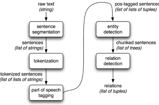
Figure 2.2 illustrates the pipeline architecture for a typical Information Ex-traction system.

Figure 2.2: Pipeline Architecture for an Information Extraction System(Bird

et al., 2009).

2.2.1 Tokenization

Tokenization is responsible for processing the text and transforming it into tokens. This process can also be known as lexer or tokenizer and is one of the first steps inNLP.

X =Casio Edifice Retrograde Chronograph Watch Men EFV-530GL-5AVUEF

where X is a product description and (x1, x2, x3, x4, x5, x6, x7) be a particular

tokenization Xt of X.

Below is a representation of the tokens from product description after using whitespace tokenization2_.

Xt= (x1, x2, x3, x4, ...) = (Casio, Edif ice, Retrograde, Cronograph, W atch, ...)

2_{The whitespace tokenizer breaks text into tokens whenever it encounters a whitespace}

(28)

2.2.2 Part-of-Speech

• Part-of-Speech (POS) Tagging is the process of assigning a token in

a corpus the corresponding part of a speech tag, based on its context and definition.

There are different techniques of POS tagging, the choice depends on the decision behind the algorithm to use for the problem in question.

Probabilistic methods are commonly used, where n-grams are specially im-portant because "picks the tag that is most likely in the given context" (Bird et al., 2009, p.204) using the previous ones to calculate.

In Figure 2.3, an example of how tagger context works using n-gram tagging.

Figure 2.3: Example of tagger context works using n-gram (Bird et al., 2009).

For this example below, we will be using the tagset of the The Penn Treebank of (Marcus et al., 1993) to show the importance of a correct meaning given to a word to determine its classification as a POS.

Tag Description

DT Determiner

IN Preposition or subordinating conjunction

JJ Adjective

NN Noun, singular or mass

NNP Proper noun, singular

NNPS Proper noun, plural

VBD Verb, past tense

VBZ Verb, 3rd person singular present

Table 2.1: Example of POS Tags from Penn Treebank Project.

Sentence 1: "The/DT earth/NN is/VBZ round/JJ"

Sentence 2: "Portugal/NNP won/VBD the/DT first/JJ/ round/NN of/IN UEFA/NNP Nations/NNPS League/NNP"

(29)

The word round is the same but the meaning is different. On the first one is a Adjective, in the second is a Noun.

2.2.3 Named Entities

Named entities is the task responsible for identifying all the noun phrases that correspond to a certain specific type (people, places, organization, dates and so on) that are mentioned in the string of text passed as input.

• Named Entity Recognition (NER) is the process of identify all named

entities. NER is a technique applied in many areas, such as question-answering, summarization, and machine translation. It is a widely used due to its effective approach that allows a reduction in search time, the algo-rithm directs its search according to the entities it finds (Nadeau and Sekine, 2007).

The appearance of characteristics previously unknown to the system is a hin-drance to their scalability.

Supervised, semi-supervised and unsupervised machine learning are the meth-ods used to recognize and tag named entities, standing out for the huge adoption of supervised and semi-supervised methods where Hidden Markov Model and Con-ditional Random Fields(CRF) have had a great performance in this type of tasks and recently for neural networks models that are the state-of-the-art (Zheng et al., 2018; Yadav et al., 2018; Dirie, 2017).

The adoption of the method involves the type of problem to be solved and based on the available dataset, however, the BIO Tagging Scheme is a chunk tag set method widely used in this type of tasks.

Tag Description

B Beginning of a chunk

I Inside of a chunk

O Outside of a chunk

(30)

In the example below we show how the system works, especially the UEFA Nations League where you can see the distinction between the beginning of the name of the organization UEFA/B-ORG and the remaining words that complete the name Nations/I-ORG League/I-ORG.

Sentence: "Portugal/B-GPE won/O the/O first/O round/O of/O UEFA/B-ORG Nations/I-UEFA/B-ORG League/I-UEFA/B-ORG"

In the previous example two named entities were recognized. Portugal was labeled as a country (GPE) and the UEFA Nations League was labeled as an organization (ORG).

Due to the fact that e-Commerce has specific named entities, we had to create custom named entities. In Section 4.1.3, the custom named entities are explained in detail, as well as the tags and values that can be obtained from the product description present in the datasets used in the development of this project.

2.3 Word Embeddings

"One-hot" encoding was the first attempt to represent text in vectors.

Each word is represented by a vector where its dimension is equal to the size of the vocabulary. A vector is composed of zeros and a single one at the position of the represented word.

The vocabulary [’cat’, ’mat’, ’on’, ’sat’, ’the’] represented in Figure 2.4, illus-trates the previous explanation.

In terms of scale and performance, this model proved to be quite weak due to the excessive amount of zeros and its inability to measure the similarity relation-ship between words.

Although there are slight changes in its representations, the structure that remains today is called word embeddings.

Word embeddings are a set of embeddings with dense vector representations that contain floating point values within each vector.

(31)

Figure 2.4: Example of a "one-hot" vector structure, from https://www. tensorflow.org/tutorials/text/word_embeddings.

The encoding in the vector is done in a way to represent the similarity relations between the words. The floating points are the weights of these relations and are automatically learned through the dataset used.

Their advantage comes from the capability of capturing the similarity of mean-ing of certain words, therefore the vector representation is close to capturmean-ing the relationship between them.

As illustrated in Figure 2.5, an embedding is represented by floating-point values.

Figure 2.5: Example of a word embedding structure with the floating-point val-ues represented, from https://www.tensorflow.org/tutorials/text/word_

embeddings.

Word embeddings techniques have evolved, and in a generalized way can be represented as two approaches: classics or contextual. (Camacho-Collados and Pilehvar, 2018)

(32)

Classic Word Embedding

The classic techniques are known to be static word embeddings because a word only has a single representation no matter the context in which it occurred.

Word representation in vector space also known as Word2Vec continues to be one of the most widely used approaches due to fact that can be represented in two model architectures: CBOW created by (Mikolov et al., 2013a) and Skip-gram created by (Mikolov et al., 2013b).

Figure 2.6 shows the two approaches of Word2Vec.

Figure 2.6: CBOW and Skip-gram models of Word2Vec. Adapted from (Camacho-Collados and Pilehvar, 2018).

FastText created by (Joulin et al., 2016) or Glove by (Pennington et al., 2014) are also some of the classic techniques that fails to capture the polysemy3_.

Typically, they perform a loop up, mapping a word to a vector.

Contextual Word Embedding

Recent techniques use language models to calculate the probability of the next word in a sequence of words using the context as a reference, thus creating contex-tualized word embeddings where it is possible to capture the semantics of words in different contexts, solving the problem of polysemy.

BERT presented by (Devlin et al., 2018) is the state of the art in NLP tasks and the fast fine tuning is its the major point. Figure 2.7, represents the architecture.

(33)

Figure 2.7: BERT model architecture. Adapted from https://ai. googleblog.com/2018/11/open-sourcing-bert-state-of-art-pre.html.

ELMO created by (Peters et al., 2018) or Flair Embeddings by (Akbik et al., 2018) has similarly to BERT the downside of being necessary a lot of computational power to perform this task.

2.4 Neural Networks

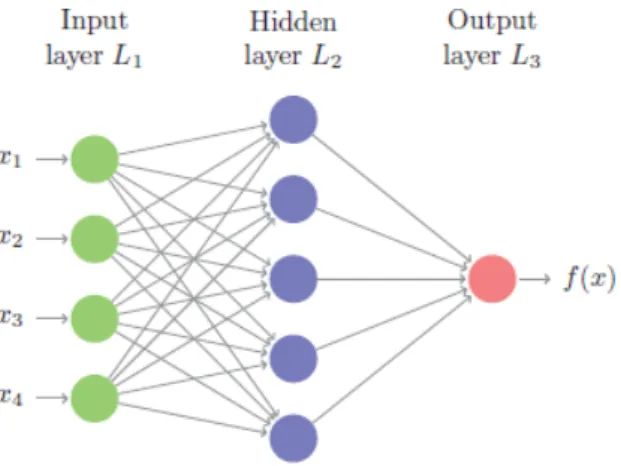
The basic architecture of a neural network is the feed-forward network, composed of several layers of neurons, where the leftmost layer in the network is called the input layer, the rightmost is the output layer and in the middle, we have the hidden layers. The design of the input and output layers in a network is often straightforward, which means that the output value of each neuron will be the input value of the next neuron, forming a single fully connected neural network (Figure 2.8).

The RNN are simply loops of feed-forward neural networks. In Figure 2.9, it is possible to observe a standard RNN. By decomposing a RNN, a chunk of the neural network is visible in the middle state, where xtis the input, tanh is the

activation function that defines the output given an input and ht is the output

value. A loop allows information to be passed from one step of the network to the next. In other words, a RNN is like a multiple copies of the same network, each passing a message to a successor.

(34)

Figure 2.8: Simple feed-forward neural network, adapted fromhttp://uc-r. github.io/feedforward_DNN

Figure 2.9: Standard Recurrent Neural Network single tanh layer, adapted from http://colah.github.io/posts/2015-08-Understanding-LSTMs/.

Considering the architecture, it is evidenced that RNN are related to se-quences and lists and hence the problem of Vanishing Gradient (VG).

The VG problem is related to the update of weights over backpropagation through time when modelling a long sequence of words, it is easily corrupted by multiplying small gradients over the sequence to the initial state. To overcome, this problem (Hochreiter and Schmidhuber, 1997) created a RNN variant called

Long Short-Term Memory(LSTM).

RNN are being overlooked by LSTM due to the high performance of their hidden state layers. It increases the complexity of the model but allows a more effective solution.

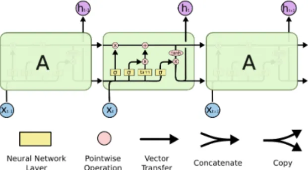
Figure 2.10 presents the LSTM architecture and how its cells works. One

determinant feature is the memory cell Ct and have the ability to influence the

storing or overwriting memories. The formula is defined in Equation 2.1.

(35)

Figure 2.10: Long Short-Term Memory architecture, adapted from http:// colah.github.io/posts/2015-08-Understanding-LSTMs/.

Each cell is composed by three important gates: forget ft, input itand output

gate ot. Those gates have a different role but they all block or pass information

based on its strength and importance, filtered by their own sets of weights. Forget gate layer has the responsibility to choose what information retain based on previous output layer ht−1and input of the current cell xt(Equation 2.2).

ft= σ(Wf · [ht−1, xt] + bf) (2.2)

The next step is the input gate layer where learns new inputs that are worth using and determines how much of the input to let into the cell state (Equation 2.3).

it= σ(Wi· [ht−1, xt] + bi)

ˇ

Ct= tanh(Wc· [ht−1, xt] + bc)

(2.3)

And the last gate are output layer where is decided what output value goes out and stored in the memory cell (Equation 2.4).

ot= σ(Wo· [ht−1, xt] + bo)

ht= ot∗ tanh(Ct)

(2.4)

Recent approaches are based on Bidirectional LSTM (BiLSTM). They are similar toLSTMs, but have advantage of accessing information in both directions. (i.e. by representing future steps, you can understand the context and eliminate ambiguity)

(36)

Also, we have theConvolutional Neural Network(CNN), which is a variation of the neural networks where the greats contributions are in the fields of computer vision and audio simply because convolution and pooling functions are used as activation functions (Figure 2.11).

Figure 2.11: Example of CNNarchitecture (Zhang and LeCun, 2015).

Sparse interactions, parameter sharing, and equivariant representations are important characteristics of convolution.

The interactions between the input and output units are quite different from traditional neural networks.

The convolution layer aims to reduce the complexity of the data entered by trying to find relevant characteristics, reducing the number of parameters and memory used allowing an increase in efficiency in the model. By limiting the num-ber of possible connections to the output, we are limiting the numnum-ber of possible parameters and indirectly the number of runtimes.

The size of the weights, also known as filter or kernel, is smaller than the input data purposely to be applied multiple times at different input points. Thus, it can scroll efficiently through the input data from left to right, top to bottom (Figure 2.12).

Equation 2.5 demonstrated the formula behind discrete convolution.

(f ∗ g)(i) =

m

X

j=1

g(j) · f (i − j) _(2.5)

Where g is the input and f is the kernel, also this formula can only be defined if we assume that g and f are defined in the integer i.

(37)

Figure 2.12: Example of sparse connectivity, convolution layer represented on top with three width kernel, in the bottom is represented a traditional matrix

multiplication, where are not sparse (Goodfellow et al., 2016).

If we use convolutions with more than one axis in the same time reference, need to use a two-dimensional kernel as represented at Equation 2.6.

(I ∗ K)(i, j) = X

m

X

n

I(m, n)K(i − m, j − n) _(2.6)

or Equation 2.7 because convolution are commutative.

(K ∗ I)(i, j) = X

m

X

n

I(i − m, j − n)K(m, n) _(2.7)

Where I is a two-dimensional image input and K is a two-dimensional kernel. As exhibited in Figure 2.13, pooling is very relevant in the composition of CNN since it allows us to give a fixed output value as well as the reduction of the dimensionality saving only the information considered useful and that stands out. It also has overfitting supervision as a characteristic and can assume the min polling layer or average polling layer, although the max polling layer is the most adopted.

(38)

Figure 2.13: Example of max pooling layer effect. Adapted from http:// cs231n.github.io/convolutional-networks/#pool.

2.5 Conditional Random Fields

Conditional Random Fields (CRF) originally proposed by (Lafferty et al., 2001) belongs to the group of discriminative classifiers, and they model the decision boundary between the different classes.

The discriminative models assume the following Equation 2.8, where Y and X are given directly from the training set.

P (Y |X) (2.8)

The model has learned the decision boundary that separates the data points by learning the conditional probability distribution. However, it needs to be effi-cient to predict a sequence computation like Equation 2.9.

ˆ

y = argmaxyP (Y |X) (2.9)

Like linear regression, the CRF also uses feature function to represent char-acteristics in data sequences.

The feature function is represented by Equation 2.10.

F (¯x, ¯y) =X

i

f (yi−1, yi, ¯x, i) _(2.10)

Where the ¯f function analyzes the entire ¯x sequence for the corresponding tags, ¯i is the current position where it is in the phrase. ¯y yi−1¯ represents the

(39)

previous positions in the tag sequence and ¯yi corresponds to the current position.

Areas such as part-of-speech tag or named entity recognition are very prolif-erating due to the need to predict the current word tag and its dependency on neighboring words and tags.

The model can assume several different graphs, our focus is on linear-chain CRF due to its structure and capability in NLP tasks.

Below is represented a linear-chain structure in the Figure 2.14and is formu-lated using Equation 2.11.

Figure 2.14: Linear chain-structuredCRFs (Wallach, 2004).

P (¯y|¯x; ¯w) = _P exp( ¯w · F (¯x, ¯y))

¯

y0_∈yexp( ¯w · F (¯x, ¯y0))

(2.11)

where the feature function described above is represented and the sum of all values over the yn _{have been normalized.}

(40)

(41)

Chapter 3 Related Work

This chapter discusses the research that has been conducted in the field of informa-tion extracinforma-tion from product for e-commerce applicainforma-tions. The chapter is divided into several sections, aiming to group the different approaches to the problem and to provide an overview of the algorithms and techniques used for each different approach.

3.1 Datasets for e-Commerce

Natural language processing tasks are quite complex, with many particularities that require large amounts of previously noted knowledge to facilitate the task. Datasets like CoNLL2003, presented by (Sang and De Meulder, 2003) or OntoNotes 5.0 by (Pradhan et al., 2013), are great drivers in the scientific advancement of

NER task.

(Uzuner et al., 2011) created I2B2 to challenge the scientific community to research and develop based on clinical records. The same happened when (Kim et al., 2003) created GENIA for the recognition of bio entities.

Researchers’ interest in e-commerce has grown. Although there are several re-searchers from large corporations such as Amazon, eBay, Walmart, Rakuten, they do not practice to disclose the datasets used, making it impossible to reproduce or use new approaches to previously proposed methods.

(42)

Table 3.1 shows a summary of the datasets, the type of attributes present, the volume of data and where they can be found.

# Dataset Name Attributes Included Sentences Available at 1 Victoria’s Secret

and Others

product name, price, brand name, de-scription, retailer, rating, style at-tributes, total and available sizes, color, ...

614,262 https://www.kaggle.com/PromptCloudHQ/

innerwear-data-from-victorias-secret-and-others# amazon_com.csv

2 Electronic Prod-ucts and Pricing Data

brand, category, merchant, name, prices, condition, source, ...

7,000 https://data.world/datafiniti/ electronic-products-and-pricing-data

3 Men’s Shoe Prices

brand, category, colors, description, features, ean, source, ...

10,000 https://data.world/datafiniti/mens-shoe-prices

4 Women’s Shoe Prices

brand, category, colors, description, features, ean, source, ...

10,000 https://data.world/datafiniti/womens-shoe-prices

5 Best Buy E-commerce NER dataset

brand, category, model name, screen size, ram, storage, price

941 https://www.kaggle.com/dataturks/ best-buy-ecommerce-ner-dataset

6 Amazon and Best Buy Elec-tronics

brand, category, colors, name, reviews text, reviews title, reviews rating, ...

7,000 https://data.world/datafiniti/ amazon-and-best-buy-electronics

7 Product details on Flipkart

url, name, category, description, brand, product specifications, ...

20,000 https://data.world/promptcloud/ product-details-on-flipkart-com

8 Fashion prod-ucts on Amazon

name, manufacturer, price, number of reviews, average review rating, cus-tomer review, category, description, product information, ...

22,000 https://data.world/promptcloud/ fashion-products-on-amazon-com

9 Abt-Buy name, description, price, manufacturer 2,173 https://dbs.uni-leipzig.de/research/projects/ object_matching/benchmark_datasets_for_entity_ resolution(Köpcke et al., 2010)

10 Amazon-GoogleProducts

name, description, price, manufacturer 4,589 https://dbs.uni-leipzig.de/research/projects/ object_matching/benchmark_datasets_for_entity_ resolution(Köpcke et al., 2010)

11 Walmart brand, upc, title, price, short descrip-tion, long descripdescrip-tion, dimensions, ...

2,554 http://pages.cs.wisc.edu/~anhai/data/corleone_ data/products/(Gokhale et al., 2014)

Table 3.1: A summary of public e-Commerce datasets.

Although there are several datasets previously shown by Table 3.1, most of them have missing values or bad catalog values.

Several researchers from large corporations such as eBay (Putthividhya and Hu, 2011), Walmart (More, 2016)(Zhang and LeCun, 2015) and Rakuten (Shinzato and Sekine, 2013) use huge datasets, different from those previously presented. They do not have the practice of disseminating the datasets, which makes their reproduction or new approaches to previously proposed methods impossible.

3.2 Attribute-Value Pairs Extraction

The AVP extraction is the problem of identifying the values for one or more attribute of any entity and many researchers have fallen into this field of investi-gation.

(Ghani et al., 2006) uses a supervised model to extract the AVP through

(43)

Chapter 3: Related Work

semi-supervised layer co-Expectation-maximization over the NB, making it pos-sible to scale the model using a limited set of labeled training data.

(Raju et al., 2009) presented an unsupervised approach to extract product attributes using ngrams to calculate the similarity between noun phrases that later is used by a clustering algorithm. Attributes are obtained through a ranking function. Although they also use ngrams, (Putthividhya and Hu, 2011) generate their training dataset via bootstrap from matching n-grams words, with dictionar-ies and posteriorly manually inspected to guarantee that they have no flaw. The result is a supervised named entity recognition pipeline that extracts attributes from product title.

(Kovelamudi et al., 2011) proposes a supervised system to extract the at-tributes of the products through the reviews made by the customers to them. To this end, they created a database of semantic relationships where they correlate the words highlighted in customer reviews and articles in Wikipedia or on the Internet. They use the support vector machine to train the model using the hand-crafted features previously highlighted. Despite using customer reviews, (Broß

and Ehrig, 2013) adopted an unsupervised approach were their system depends

on heuristic filtering to obtain candidates from customer reviews. Highlight that sentiment expressions are detected through a hand-crafted compound lexicon. All terms referring to the product or brands are removed through a stop word list previously created.

(Shinzato and Sekine, 2013) applies an unsupervised model to automatically create a Knowledge Base (KB) from product pages tables. Having already built aKB, they used it to create a new set of annotated data. The model chosen was the CRF and an AVP layer is used for each category. Similar to the previous approach, (Charron et al., 2016) used consumer patterns along with subtrees-based extraction and information listing to create the annotation of data-driven products. It is an end-to-end unsupervised architecture.

Having made a similar approach to (Shinzato and Sekine, 2013), (Bing et al., 2016) proposed to extract attribute value in an unsupervised way that was trained by a hidden CRF model. Their method uses latent Dirichlet allocation (Blei et al., 2003), deconstructing the sentence and finding the unknown concepts crucial to popular features, assigning to a domain.

(44)

3.3 Neural Sequence Labeling Models

NER is a close research area to our problem and has been widely addressed in scientific literature. While the first systems for recognizing names were based on pattern matching rules and pre-compiled lists of information, the research com-munity has since moved towards employing machine learning methods for creating such systems (Goyal et al., 2018).

Models used for predicting Named entities in text sequence faced the struc-tured prediction problem and can be broadly classified into supervised, semi-supervised and unsemi-supervised models.

The supervised learning requires a lot of annotated data and the costs of their creation contribute to choose alternative learning methods.

Semi-supervised is an alternative that needs a small labeled training set and a huge corpus of unlabeled data.

Unsupervised learning is the opposite of the supervised learning approach and is also an alternative. It works without any label data and its task is to find patterns in the unlabeled data. Below, we detailed some approaches.

(Huang et al., 2015) is a pioneer in the implementation of theBiLSTM-CRF model, where it represents each word of the sentence vectorially, and through a hand-craft rules system, the vector goes to the CRF layer. The hand-craft rules system is to handle spelling and context features like uni-grams, bi-grams and tri-grams.

(dos Santos and Guimarães, 2015) proposes a deep neural network that uses char embeddings and word embeddings jointly as input to the convolution layer. They framed their approach was a sequential classification problem. It also uses a dropout layer on BiLSTMoutput nodes to reduce model overfitting. The output as normalized after the Viterbi layer found the most probably tag for word. (Chiu

and Nichols, 2016) also used a hybrid model where CNN receives the junction

between character and word embedding. BiLSTM applies each iteration with

a linear layer and a softmax layer to calculate the log probabilities of each tag category. It also uses a lexicon with the BIOES tag as an annotation.

(45)

Chapter 3: Related Work

is responsible for outputting the correct tag by maximizing the matrix transition scores. Similarly, (More, 2016), (Rei, 2017), (Ma and Hovy, 2016) and (Yadav et al., 2018) propose an identical system where (More, 2016) use distant supervi-sion technique with a rule-based strategy to obtain the dataset. Also, normalize at the end to ensure the existence of unique value. (Rei, 2017) present aBiLSTM capable of multitasking and encouraged to discover new features and uncheck an "O" tag so as not to submit the template. Additionally, (Ma and Hovy, 2016) present a CNN layer similar to (Chiu and Nichols, 2016) except that the input data of the model presented by them are only character embeddings and these use a junction char + word embeddings. It also applies a dropout layer to the data input on CNN. (Yadav et al., 2018) shown a similar approach, but learns the structure and their n-gram suffix and prefix of each word.

(Dirie, 2017) proposed a similar approach to (Yadav et al., 2018), where he addresses character-level and word-level with BiLSTM and word-embedding trains him in an unsupervised way through skip-gram. In the last layer, it ap-plies aCRFMultiplex layer which allows an attribute-by-attribute tagging policy capturing previously unknown attributes more efficiently.

(Shen et al., 2017) aims to reduce the amount of tagged data required to train the model while maintaining its quality. For this, it uses deep learning along with active learning. In order not to overload the system with model retraining, it adds the new data along with the old one and updates the neuronal network weights to a lower number of epochs. The active learning layer select sentences that have been predicted with the lowest normalized size log probability. TheCNN-CNN -LSTM architecture works with a character-level convolutional encoder, another convolutional encoder for words, and the final layer is LSTM as a decoder tag.

(Zheng et al., 2018) frames the problem as a sequence tagging task where it uses a BiLSTM-CRF attention model. The tagging strategy adopted is similar to (Lample et al., 2016). It uses an active learning strategy using the flip method tag to drastically reduce the need for manually annotated data.

(46)

Authors Features Architecture Resume Structure Tagging

Embeddings Datasets Used (Huang

et al., 2015)

Yes BiLSTM output vector + hand-craft rules features vector connected to CRF

CRF (Collobert et al., 2011) pre-trained with 50-dimensions CoNLL2000 + CoNLL2003 (dos San-tos and Guimarães, 2015)

Yes char-level + word-level embeddings as input to CNN, minimize the negative log-likelihood with stochastic gradient descent

Sentence-level log-likelihood

pre-trained word embeddings Skip-gram + char-level embeddings ex-tracted with a CNN SPA CoNLL2002 + HAREM I (Chiu and Nichols, 2016)

Yes char + word embeddings as input to BiLSTM layer, BiLSTM output with dropout decoded by linear layer + log-softmax layer into log-probabilities for each tag category

(Collobert et al., 2011) pre-trained with 50-dimensions + char-level embeddings extraction with a CNN CoNLL2003 + OntoNotes 5.0/CoNLL2012 (Lample et al., 2016)

No char + word embeddings as input to BiLSTM layer, CRF receives the out-put vector to decode label sequence

CRF pre-trained word embeddings skip-n-gram + char-level embeddings extrac-tion with BiLSTM

CoNLL2002 + CoNLL2003 (Rei, 2017) No BiLSTM with additional language

modeling to predict sequence label us-ing softmax layer as output.

pre-trained word embeddings word2vec with 300-dimensions + trained word embeddings PubMed + PMC with 200-dimensions FCE + CoNLL2014 (Ma and Hovy, 2016)

No jointly char + word embeddings as in-put to BiLSTM layer, CRF receives the output vector to decode label sequence

CRF pre-trained word embeddings Glove with 100-dimensions + char-level em-beddings extracted with CNN

WSJ + CoNLL2003 (Yadav

et al., 2018)

Yes char-level embeddings as input to BiL-STM layer + BiLBiL-STM output vector with word-level embedding as input to BiLSTM + CRF input fedded by BiL-STM word-level output vector

CRF char-level embeddings extraction with BiLSTM + pre-trained word embed-dings Fasttext with 300-dimensions + pre-trained word embeddings Glove with 100-dimensions + pre-trained word embeddings PubMed with 300-dimensions CoNLL2002 + CoNLL2003 + DrugNER (MedLine + DrugBank) + I2B2 (Dirie, 2017)

No char-level embeddings as input to BiL-STM layer + BiLBiL-STM output vector with word-level embedding as input to BiLSTM + CRF Multiplex input fed-ded by BiLSTM word-level output vec-tor

CRF char-level embeddings extraction with BiLSTM + trained word embeddings Skip-gram

Rakuten

(Shen et al., 2017)

No CNN output vector as input jointly with word embedding into CNN + LSTM receives CNN output vector and decode label sequence through LSTM layer + active learning to help reduce reliance on tagged training data

char-level embeddings extraction with CNN + trained word embeddings word2vec OntoNotes 5.0 + CoNLL2003 (Zheng et al., 2018)

No BiLSTM-CRF with attention model + active learning using flip tag method

CRF pre-trained word embeddings Glove with 100-dimensions

Amazon

(47)

Chapter 4 Attribute-Value Pairs Extraction

Following the related work and taking into account the investigation methodol-ogy used, it follows the stage of developing a solution considering all the facts previously reported.

Figure 4.1shows the pipeline used in our model and all the steps required to develop it.

Figure 4.1: Pipeline of our approach.

In the following sections you will find the explanation of each step and the reason for the decisions taken.

(48)

4.1 Datasets

Due to the difficulty in getting an e-Commerce dataset that contained the infor-mation about the products (e.g. product title or product description) properly labeled with the part-of-speech or/and named entities tag, we felt the need to create a dataset from scratch.

The creation of the datasets belongs to the field of research Web Data Ex-traction where the structure of the HTML mark-up language present in the web pages was used as an advantage for the extraction.

Not being the focus of this project and after a brief literary review on the theme in question (Ferrara et al., 2014), we decided to use as a technique of information extraction a tree-based approach.

The DOM (Document Object Model) is the representation of the HTML pages in plain text, where the elements are represented through the HTML tags as well as the text present on each page. The tree structure is easily understood, with each HTML tag representing a node. These structures are called DOM Tree.

The technologies used in the development of this artifact to obtain the neces-sary data for the construction of the dataset was the java programming language, using the Selenium library1 to interact with the web page in an automated way. Apache POI2 was also used to create, write and modify the XLS/XLSX spread-sheets to save all information extracted.

Being our focus on the e-Commerce websites, where the product listings are structured dynamically, it is necessary to use the existing structural similarity in the DOM trees to extract efficiently and effectively without human iteration.

The product listings are represented in lists, where the iteration with the various products is done through an iterator. At each iteration, all the information about the attributes and values of each product is obtained through the tables. The change of page for a new listing is made when there are no more products in the current list.

1_{https://www.seleniumhq.org/download/} 2_{http://poi.apache.org/download.html}

(49)

Chapter 4: Attribute-Value Pairs Extraction

We created three new datasets, two belong to the fashion sector and the other is a junction of the sectors: home, furniture, appliances, sports, fitness and outdoors.

In order to ensure the confidentiality of the websites involved in this process, we will now call the dataset with limited data of Jewels (2214 products), the dataset that contains a large amount of products of Fashion (21775 products) and the dataset that is from a different sector than fashion of HomeDecor (250 products).

4.1.1 Datasets Structure

We decided to opt only for the inclusion of product descriptions because they already contain the information on the title and are an aggregator with more information that can be extracted.

We created three datasets with the concept of testing the generalization be-tween datasets of different categories and sizes without having been previously trained.

Jewels dataset is rather limited, contains only and exclusively 2214 products related to the jewelry industry where the descriptions are mostly structured ( Fig-ure 4.2).

Figure 4.2: Example of a product description from Jewels dataset.

In creating the Fashion dataset, we paid attention to the two important par-ticularities that we wanted to achieve. A very significant number of descriptions compared to Jewels dataset and the insertion of three new categories within the same sector to perform correlation tests.

(50)

Please note inFigure 4.3that the product descriptions of the Fashion dataset come from the brands themselves. It is notorious the difference in structuring compared to Jewels, where the raw text of the Fashion will be an added value for the diversification of the model.

Figure 4.3: Example of a product description from Fashion dataset.

The HomeDecor dataset was created with the perspective of being the most different from Jewels and Fashion and in its genesis is the concern of the diversity of the tests, with the vast majority of its 250 products being disparate and different from the fashion sector.

The descriptions of their products are unstructured and with fewer standards of the three datasets in question. Figure 4.4 visually demonstrates what we ex-plained above.

Figure 4.4: Example of a product description from HomeDecor dataset.

This dataset was conceived for inference task, where the main objective is to known new words and recognize those already known.

4.1.2 Annotation

After the extraction of the information and the creation of the dataset, it is now important to proceed with the labelling of the data taking into account the custom named entities.

Based on the related work, we adopt the distant supervision that will be explained below.

(51)

Chapter 4: Attribute-Value Pairs Extraction Distant Supervision Model

Due to limited human capacity and the high annotation costs of large datasets, researchers have felt the need to adopt new approaches and techniques for rapid, effective and low false-positive labeling.

We adopted the use of the distant supervision model after reading several identical projects(Dirie, 2017).

The distant supervision model starts with the existence of datasets or external sources of information(Mintz et al., 2009; Shinzato and Sekine, 2013; Wu and Weld, 2007) and uses them to complement the relationships needed to label the dataset, thus making it possible to have a large set of training data, guided in the annotation process.

Assuming that the sites where the information was extracted contained the correct information about the value attribute pairs in their tables, as shown in Figure 4.5 and Figure 4.6, we used our previously created csv file as a reliable external source to guide the annotation.

Figure 4.5: Example of a product description extracted from product page

For each previously extracted product description, a word-by-word annotation is made with the attribute values from the product table. Whenever the description word and attribute value are equal, the word is tagged with "B-*" and followed by the tag, indicating the beginning of this attribute. If the attribute value contains more than one word, this indicates that the next word in the description also has the same attribute. Since the previous word is of the same attribute, we use "I-*" as the prefix followed by the tag. All other words in the description that are not equal to any attribute values are labeled "O".

(52)

Figure 4.6: Example of a attribute-values extracted from the product page

4.1.3 Custom Entity Tagging

In Section 2.2.3, we introduce of the named entity recognition task where we described its importance in the recognition of entities as well as the possible an-notation schemes.

The labels appear as a facilitator in the task of recognizing entities present in the input text and the entities present in e-Commerce websites are quite different from the entities present on CoNLL-2003 (Tjong Kim Sang and De Meulder, 2003). The difference in contexts leads us to create our entities to correctly label the products.

As mentioned in Section2.2.3, the tag scheme is very important in the recog-nition of entities. According to (Reimers and Gurevych, 2017), BIO stands out and is the most recommended choice for tasks related to entities.

Table 4.1 shows an example of the BIO annotation scheme that we adopted

to encode the different entity tags, using the example of Figure 4.7.

(53)

Figure 4.7: Example of product description with custom entities tags.

Tag Label Meaning Example Given

B-B Beginning of a Brand Casio

I-B Inside of a Brand Edifice

B-G Beginning of a Gender men

B-PC Beginning of a Product Color brown

B-PC Beginning of a Product Color rose

I-PC Inside of a Product Color gold

B-PM Beginning of a Product Material leather

B-PT Beginning of a Product Type watch

B-WR Beginning of a Water Resistance 10

I-WR Inside of a Water Resistance ATM

I-WR Inside of a Water Resistance /

I-WR Inside of a Water Resistance 100

I-WR Inside of a Water Resistance M

Table 4.1: Custom Entity Tag with BIO tag scheme using Figure 4.7 as ex-ample

Quality Concerns

Tasks such as data tagging are undergoing this change due to the difficulty in arranging large datasets to train natural language models.

The issue of quantity for quality is well suited to the problem.

Our approach to the problem was initially via distant supervision and then we manually check the quality of the data for possible annotation errors.

(54)

4.2 Supervised Learning Model

After a brief general introduction and visualization of the general pipeline of the artifact (Figure 4.1), we will now discuss in detail the algorithms used as well as their main features.

We can see the structure of our model as being divided into three layers, where the first layer is CNN, the second is BiLSTM and the last is CRF.

We used a CNN-BiLSTM-CRF that is capable of transfer learning based on (Ma and Hovy, 2016) approach whereFigure 4.8 exhibits the interaction between the algorithms.

Figure 4.8: Architecture of our neural network (Ma and Hovy, 2016).

4.2.1 Convolutional Neural Network

After a brief introduction of the operation of the CNN algorithm in Section 2.4, where convolution and pooling concepts have been demonstrated and explained, we intend with this chapter to describe in detail how and why theCNNalgorithm is being used in NLPtasks and its relevance in the current state of the art.

(55)

Our approach contemplates a convolution and max pooling layer that tries to capture the spelling and morphological characteristics of words or words in the context of the sentence, thus allowing rare or misspelled words as well as prefixes and suffixes words to be recognized through the use of language models based only on the spelling of the word and its similar vectors (Gridach, 2017). This

character-level layer and can be LSTM-based or CNN-based. We choose a CNN-based

approach according to (Zhai et al., 2018, p.38), "the models using CNN-based character-level word embeddings have a computational performance advantage, increasing training time over word-based models by 25% while the LSTM-based character-level word embeddings more than double the required training time."

Figure 4.9 illustrates how the text is represented as a matrix where each row of the matrix corresponds to a character.

Figure 4.9: Character-level information encode into Convolutional Neural Net-work (Ma and Hovy, 2016)

The efficiency in terms of representation makes convolution filters achieve good representations automatically without having to represent the entire vocab-ulary. Thus, it can capture the features similarly to n-grams but representing it in a more compact way and without suffering from its limitations.

Word Embeddings

We have chosen not to use an unsupervised word embedding for the simple reason that unsupervised models are only adequate if the dataset used for training has an appropriate size.

(56)

The word embeddings chosen were trained using structural information from dependency graphs and according to (Komninos and Manandhar, 2016, p.1498), "the dependency-based word embedding largely improved the performance for semantic relation identification".

The character embeddings + word embeddings approach used by us after (Ma and Hovy, 2016) has empirically been shown that will bring better results to the final model.

Considering the points above, the concatenation between the embeddings gen-erated from character-level with word embeddings are the input of theBiLSTM layer.

4.2.2 Bidirectional LSTM

(

BiLSTM

)

BiLSTM is the extension of the LSTM referenced in Section 2.4. It uses past

information as well as future information to predict.

In other words, BiLSTM is a set of two layers of LSTM where one layer processes the information from left to right (forward) and the other layer, from right to left (backward).

Figure 4.10 shows the structure ofBiLSTM.

Figure 4.10: Architecture of Bidirectional Long-Short Term Memory. Adapted fromhttp://colah.github.io/posts/2015-09-NN-Types-FP/

(57)

4.2.3 Conditional Random Fields

(

CRF

)

After a brief introduction of the CRF equations in Section 2.5, where we present the feature function and the linear-chain CRF, we will now present the full ex-panded linear-chain CRF inEquation 4.1.

P (¯y, ¯x; w) = exp( P i P jwjfj(yi−1, yi, ¯x, i)) P y0_∈Y exp( P i P jwjfj(y 0 i−1, y0i, ¯x, i)) (4.1) whereP

i is the length of sequence x,

P

j is the sum over all feature function,

wj is the weight for given feature function and

P

y0_∈Y is the sum over all possible

tag sequence.

The previous equation is represented globally by the feature function fk by k,

where it makes the sums of all the features functions by the different n transition states existing in ¯y. Thus, the entire sequence is mapped in F (¯x, ¯_{y) ∈ R}d

The CRF is the last layer of the model and this makes it possible to add constraints to the final labels to ensure their validity.

The constraints are automatically applied and learned, based on the set passed during the training phase.

The CRFlayer receives an matrix (number of words in a sentence multiplied by the number of possible labels for each word) with the Pij results where jth is

the probability that the tag is the correct ith _{word in the sentence. For better}

understanding, Figure 4.11 represents the dynamics between the BiLSTM and

CRF layers, matrix with the probabilities and the CRF layer giving the output results that maximize the score function.

There is also a transition matrix that represents the probability of transition between tags. It allows us to get information about the veracity of the model, conclude unlikely transitions as well as outliers. An example is that transitions from I-* to B-* are never possible in practice and if the weights are found to be positive and high, it is a sign of incongruity in the model.

(58)

Figure 4.11: Emission score from BiLSTM layer. Adapted from https:// createmomo.github.io/2017/09/23/CRF_Layer_on_the_Top_of_BiLSTM_2/

The score function for predicting a sequence is given by the sum of the tran-sition between the current state tag and the next state tag, along with the prob-ability from BiLSTM of being the correct tag for the current word as shown in Equation 4.2. Pscore(y) = n X i=0 Tyi,yi+1+ n X i=1 Pi,yi (4.2)

which is then used in Equation 4.3 to find a single tag for each word so that the junction of all the single tags gives the highest value of the joint probability.

(59)

4.2.4 Summary

Our approach takes into account the approaches presented in the related work (Ma and Hovy, 2016; Dirie, 2017). The structure is CNN-BiLSTM-CRF where CNNdeals with the character-level that together with the word-embedding is the input of the BiLSTMlayer, that through its powerful ability to analyze sentence sequences has as output the matrix of probabilities of tags for each word. Also, CRF that together with the emission matrix received from BiLSTM, gives the tag sequence that maximizes the score function.

(60)

(61)

Chapter 5 Experimental Settings and

Evaluation

5.1 Experimental Settings

In this chapter we explain in detail the composition of the datasets, the metrics used to evaluate the model, and the components required to run the model.

As described in Section4.1, we created three datasets to test the generalization capability of the model.

Table 5.1 shows the structure of each dataset as well as the categories it contains and their size.

Dataset Categories Size

Jewels Jewelry 2214

Fashion Clothing, Shoes, Accessories & Jewelry 21775 HomeDecor Home, Furniture & Appliances + Sports & Outdoors 250

Table 5.1: Datasets Structures

For a better perception of the diversity between types of products within the dataset, we present the following figures.

Figure 5.1 and Figure 5.3 show that there is a lot of data disparity between certain types of products, however, it was made purposely to realize how the system interacts and reacts to this type of adversities.

(62)

Figure 5.1: Distribution by product type of the Jewels dataset

Figure 5.2: Distribution by product type of the Fashion dataset

Figure 5.3: Distribution by product type of the HomeDecor dataset

In this project we focus on only 6 classes and 11 labels. Note that inFigure 5.4 does not appear water resistant because this class only belongs to the Fashion dataset, as such, there would be no comparison term. We do not use the I-G tag because there is no genre with more than one word. Figure 5.4 shows the distribution between the various classes by the 3 dataset.

(63)

Chapter 5: Experimental Settings and Evaluation

Figure 5.4: Distribution of dataset tags

Through the image, we observe that the dataset Fashion and Fashion+ contain much more data and their distribution prevails in the classes B-PT and B-B.

Our tests will use the three most commonly used metrics: Precision, Recall and F1-Score. Table 5.2 represents the meaning of True Positive, False Positive, and False Negative in the context of entity recognition.

Metrics Meaning in this context Gold Label Predict Label

True Positive (TP) Token and predicted token are positive B-B B-B False Positive (FP) Token are negative but predicted token is positive O B-B False Negative (FN) Token are positive but predicted token is negative B-B O

Table 5.2: Meaning of metrics

True negative happens when the token and its prediction are both negative. In this case, tags being equal means they are well labeled and its fits True Positive, however, due to the high hit rate and the direct relationship with the input data, we chose not to sum it to make the results more realistic.

The precision formula is Equation 5.1, the recall is Equation 5.2 and the f1-score inEquation 5.3.

P recision = T P

(64)

Recall = T P

T P + F N (5.2)

F 1 − Score = 2 × P recision × Recall

P recision + Recall (5.3)

5.1.1 Experimental Setup

Our model was made in the python1 programming language in version 3.6 on

Ubuntu 18.042 _{operating system. We use keras 2.2.0}3 _{and tensorflow 1.8.0}4 _as

backend.

One of the initial problems felt was the incompatibility of library versions together with Ubuntu and CUDA drivers5_{, and it is really necessary to be aware}

of version compatibility when creating or reusing an existing model. We use one GeForce GTX 1080 Ti to run the model.

Model configuration hyperparameters are very important and have a real im-pact on model evaluation. In order to maximize performance, we use the best settings for sequential labeling tasks, according to (Reimers and Gurevych, 2017).

Table 5.3 shows a list of the hyperparameters used by model.

Parameter Selected Value

Dropout 0.25 Classifier CRF LSTM-Size 100 Optimizer Adam miniBatchSize 32 charEmbeddings CNN charEmbeddingsSize 30 charFilterSize 30 charFilterLength 3

Table 5.3: Hyperparameters used in the model

1 https://www.python.org/downloads/ 2_{https://ubuntu.com/download/desktop} 3_{https://pypi.org/project/Keras/2.2.0/} 4_{https://pypi.org/project/tensorflow/1.8.0/} 5_{https://developer.nvidia.com/cuda-92-download-archive}

Attribute-value inference using deep neural networks

University Institute of Lisbon

Department of Information Science and Technology