Estimating Bankruptcy Using Neural Networks Trained with Hidden Layer Learning Vector Quantization

Estimating Bankruptcy Using Neural Networks Trained

with Hidden Layer Learning Vector Quantization

João C. Neves* Armando Vieira **

*

Professor of Finance and Control, ISEG School of Economics and Management, Portugal Visiting Professor, HEC School of Management, France

**

ISEP – Dep. Física and Computational Physics Centre, Universidade de Coimbra, Portugal.

Abstract

The Hidden Layer Learning Vector Quantization (HLVQ), a recent algorithm for training

neural networks, is used to correct the output of traditional MultiLayer Preceptrons

(MLP) in estimating the probability of company bankruptcy. It is shown that this method

improves the results of traditional neural networks and outperforms substantially the

discriminant analysis in predicting one-year advance bankruptcy. We also studied the

effect of using unbalanced samples of healthy and bankrupted firms.

The database used was Diane, which contains financial accounts of French

firms. The sample is composed of all 583 industrial bankruptcies found in the database

with more than 35 employees, that occurred in the 1999-2000 period. For the

classification models we considered 30 financial ratios published by Coface1 available

from Diane database, and additionally the Beaver (1966) ratio of Cash Earnings to

Total Debt, the 5 ratios of Altman (1968) used in his Z-model and the size of the firms

measured by the logarithm of sales. Attention was given to variable selection, data

pre-processing and feature selection to reduce the dimensionality of the problem.

JEL Classification Numbers: G33; C45

Keywords: Bankruptcy Prediction; Neural Networks; Discriminant Analysis; Ratio Analysis

*

Corresponding author: João C. Neves, Rua Miguel Lupi 20, 1200-078 Lisboa, Portugal.

jcneves@iseg.utl.pt Tel: (351) 213925926; Fax: (351) 213922808.

Acknowledgments : The authors wish to acknowledge HEC School of Management and the financial

support granted by the Fundação para a Ciência e a Tecnologia (FCT) and the Programa POCTI.

1 _{Coface is a credit risk provider in France that offers the Conan-Holder bankruptcy score, a score based}

1. Introduction

Financial distress prediction is of extreme importance for banks, insurance firms,

creditors, and investors. The problem is stated as follows: given a set of parameters,

mainly of financial nature, which describes the situation of a company over a given

period, and eventually some macro-economic indicators, how can we predict if a

company may become bankrupt during the following year?

Since the work of Beaver (1967) and Altman (1968) there has been

considerable interest in using financial ratios for predicting financial distress in

companies. Using univariate analysis, Beaver concluded that Cash Earnings to Total

Debt was the best ratio for signalling bankruptcy and Altman (1968, 1977) pioneered

the use of multiple discriminant analysis in predicting bankruptcy. Since then,

discriminant analysis has become a standard approach for predicting financial distress.

However, it has been criticised due to its restrictive assumptions (Eisenbeis, 1977;

Altman and Eisenbeis, 1978; Scott, 1978; Karels and Prakash, 1987) as it requires a

linear separation between the distressed and healthy firms and the ratios are treated as

independent variables.

Non-linear models, such as the logit (Martin, 1977; Zavgren, 1985) and the

probit (Amemiya and Powell,1983), were used not only for classification but also for

estimating the probability of bankruptcy (McFaden 1976; Press and Wilson, 1978;

Ohlson, 1980 and Lo, 1986). However, these models also contain several limitations.

First the choice of the regression function is a strong bias that restricts the outcome.

Second, these methods are very sensitive to exceptions, which are very common in

bankruptcy prediction with atypical firms seriously compromising the predictions. Third,

most of the conclusions, like the confidence intervals, have an implicit Gaussian

distribution, which does not hold for many cases. Although these methods may achieve

Non-parametric models (Stein e Ziegler, 1984 and Srinivasan and Kim, 1987) or

linear programming (Gupta, Rao and Bagchi, 1990) have also been applied for

bankruptcy classification, while a more recent avenue of research is the use of neural

networks. Marose (1990), Barker (1990) and Berry and Trigueiros (1990) show that

neural network is a complementary tool for the credit risk classification problem. Udo

(1993) and Tsukuda and Baba (1994) show a higher overall efficiency of artificial

neural networks (ANN). However, they did not present any statistical test for the

predicted accuracy. Several authors (Coats and Fant, 1993; Wilson and Sharda, 1994;

Yang, 1999; Tan and Dihardjo, 2001) found that ANN is a promising and robust

technique that outperforms discriminant analysis in bankruptcy prediction. Results are

however not conclusive as Altman, Marco and Varetto (1994) conclude that neural

networks have lower generalization capability compared with traditional discriminant

analysis, even if they are more effective at the end of learning cycle. All authors agree

on the need for further research on new network topologies, training algorithms,

learning methods, and combining techniques to achieve higher predictive capabilities.

In this work we present a modification of a recent neural network method,

Hidden Layer Learning Vector Quantization (HLVQ), and analyze its efficiency against

traditional neural network methods and discriminant analysis models, using a sample of

French companies. This database is larger than most used in previous studies, which

is a factor for improving the results.

The next section describes artificial neural networks in general and Section 3

presents the HLVQ method and how it is used to correct the output of a multilayer

preceptron. Section 4 discusses the methods used for assessing the predictive

capabilities of neural network and introduces a modification of the performance

measure to evaluate the efficiency of early warning models proposed by Korobow and

Sthur (1985). This section also describes the methods and criteria used on the multiple

and HLVQ in particular, for the classification of the sample firms. Section 5 describes

the data used in the research, Section 6 presents the results, and finally Section 7

contains the conclusions.

2. Artificial Neural Networks

Artificial Neural Networks (ANN’s) are a set of algorithms inspired by the human brain’s

distributed architectures and parallel processing capabilities. ANN’s are essentially

multiple regression machines capable of learning directly from examples, requiring

almost no prior knowledge of the problem. Data classification can be considered a

regression problem, finding a function that maps an input into the corresponding class

that minimises the misclassification rate. ANN’s have intrinsic non-linear regression

capabilities that make them highly competitive on difficult classification problems

(Bishop, 1996).

The main advantage of ANN for the analyst is the reduction in unnecessary

specification of the functional relation between variables. They are

connectionist-learning machines where knowledge is imbedded in a set of weights connecting arrays

of simple processing nodes called neurons. While ANN requires little knowledge of the

problem, it is crucial to have large sets of “good quality” examples to properly train the

network, i.e., representative and error-free data.

Classification of high dimensional data is a difficult task for statistical techniques,

and for ANN as well, due to the well-known curse of dimensionality. The cause of this

problem is due to data sparseness as the dimensionality of search space increases. If,

for instance, a data point is characterized by 10 variables, each quantized in 10 states,

the number of possible configurations of the input state is 1010 and a large set of

training data will be necessary to cover this huge search space. Every time a new

is a pessimistic estimate as most variables are correlated and the regression functions

are smooth enough so that a reasonable estimate can be achieved from few points.

In general, training a network requires very large data samples, which may be

difficult to obtain for the bankruptcy problem. For the bankruptcy prediction problem it is

dubious to extract conclusions from a neural network trained with one or two hundred

observations, as was reported by some authors previous mentioned in the literature

review. As a rule of thumb the neural network should have a number of connection

weights not much higher than 1/10 of the sample size available for training. In this work

we use between 1 000 and 2 000 cases corresponding to 100 and 200 weights.

Learning can be either supervised or unsupervised. Although the former is always

preferable, sometimes the latter is used as a clustering algorithm to reduce the

complexity of the problem. In neural networks supervised learning is usually performed

by Multi-Layer Preceptrons (MLP) with a single hidden layer. The most common

method of training is back-propagation with a momentum term. Although other training

algorithms are available, in most situations the results are hardly distinguishable.

The error function used is the Sum of Square Error (SSE):

(

)

∑

−

=

n

n n

y

t

E

2

2

1

where are the target values (0 or 1) and the actual outputs of the network. The

unipolar activation function was used for the output.

n

t

y

n

Interpretation of the ANN output

Data classification is based on a winner-take-all strategy applying the following criteria

to the neural network output:

⎩

⎨

⎧

=

→

<

=

→

>

0

5

.

0

1

5

.

0

y

y

where 1 means a bankrupted and 0 a healthy firm.

There are two types of errors in classification problems. Type I error is the

number of cases classified as healthy when they are observed to be bankrupted (N10),

divided by the number of bankrupted companies (N1):

1 10

N

N

e

_I

=

.

(1)

Type II error is the number of companies classified as bankrupted when they

are observed to be healthy (N10), divided by the total number of healthy (N0):

0 01

N

N

e

_II

=

. (2)

If the output node has a sigmoid transfer function and the error function is the

sum of square errors, the output of the neural network can be directly assigned to a

membership probability (Bishop, 1996). Note however, that this interpretation is only

valid in the context of an infinite number of training data. In general the outputs of the

neural network cannot be used as a reliable estimator of the true class membership

probability, particularly when data is scarce.

3. HLVQ – Hidden Layer Vector Quantization

In classification problems, when categories are too similar, both Learning Vector

Quantization (LVQ) and Multi Layer Perceptrons (MLP) have weak performance

(Michie et al., 1994). The Hidden Layer Learning Vector Quantization (HLVQ) algorithm

was recently proposed to address this problem (Vieira and Barradas, 2003). In this

method LVQ is applied to the hidden layer of a MLP, thus combining the merits of both

approaches. HLVQ is particularly suitable for classification of high dimensional data.

The method is implemented in three steps. First, a specific MLP for the problem

extract code-vectors wci corresponding to each class ci in which data are to be

classified. These code-vectors are built using the outputs of the last hidden layer of the

trained MLP. Each example,

x

i, is classified as belonging to the class ck with the

smallest Euclidian distance to the respective code-vector:

) ( min w h x

k cj

j −

= (3)

where h is the output of the hidden layer and

⋅

denotes the usual Euclidian distance.

The third step consists of retraining the MLP with two important differences.

First the error correction is applied not to the output layer but directly to the last hidden

layer, thus ignoring from now on the output layer. The second difference is that the

error applied is a function of the difference between

h

(

x

)

and the code-vector,

w

ck, of

the respective class ck to which the input pattern x belongs. We used the generalized

error function:

(

)

∑

−

=

i

i k c

h

x

w

E

β

β

(

)

1

1

(4)

The parameter β may be set to small values to reduce the contribution of outliers.

After training a new set of code-vectors,

i c i c new

c w w

wi = +∆

(5)

is obtained according to the following training scheme:

)

)(

(

c_i

i

c

t

x

w

w

=

−

∆

α

if x ∈ class ci ,

0

=

∆

w

ci if x

∉class

ci

(6)

The parameterα (t) is the learning rate, which should decrease with iteration t to

process. The method stops when a minimum classification error is found on the test

set.

The distance of given example x to each class prototype is obtained by:

i

c i

h

x

w

d

=

(

)

−

(7)

HLVQ was applied with success in classification problems with high

dimensional data, like Rutherford BackScattering data analysis (Vieira and Barradas,

2003).

MLP output correction using HLVQ

One of the major drawbacks of MLP’s is their poor out-of-sample performance in

regions not covered by the training data, particularly frequent in high dimensional data.

In order to alleviate this situation we propose the following method to correct the MLP

output for out-of-sample or test set data.

Each example to be tested, xi, is included in the training set and the neural

network retrained. Since the real situation of the company is unknown, we first consider

it as class 0 (healthy) and determine the corresponding output y₀(xvi)= y₀i as well as

the respective distances to each class prototype obtained by HLVQ,

) ) ( , ) ( ( ) ,

( ₀0 ₀1 _{0 0 0 1}

0 c i c i c c i w x h w x h d d

dr = = r − r − (8)

Then the network is retrained considering now the test example as class 1

(bankrupted). The new output

y

1

(

x

i

)

=

y

1i

v

and the respective distances to the

prototypes are then obtained:

) ) ( , ) ( ( ) ,

( ₁0 ₁1 _{1 0 1 1}

1 c i c i c c i w x h w x h d d

The correct output is chosen following a heuristic rule:

if

i i

y

y = ₀ d₀c0 <d₀c1

if .

i i

y

y

=

_{1 1}c1 ₁c0

d

d

<

We call this method HLVQ-C. If the example is a clearly bankrupted or healthy

company the neural network output is a value close to 1 or to 0, respectively and in

both cases the correction applied after retraining is small. However, when the output is

close to 0.5 large corrections may occur. The most important corrections to the MLP

output correspond to companies with uncommon financial records for which the training

set contains few similar situations. Through a detailed analysis we found that the

majority of corrections are consistent with the most relevant ratios.

4. Assessment of predictive capabilities of ANN

The quality of a neural network is measured by its generalization capability and

robustness. To avoid the serious problem of over-fitting and validate the results of the

network on the out-of-sample data, several procedures were implemented.

Weight averaging

As training evolves, the network weights converge to a set of values that minimizes the

classification error. However, if data is insufficient to encompass the weights,

oscillations may occur and the training may stop in a local minimum. To circumvent this

problem, instead of using the final set of weights, we used the average of the last 5

best training epochs. This simple procedure proved to be effective to avoid errors on

the test set due to the presence of uncharacteristic cases, i.e., companies with a set of

Generalization

Generalization is a measure of the performance of the network on unobserved cases.

The generalization capability of a neural network is often estimated by separating the

dataset into two groups: a training set and a test set. The network is trained with data

from the training set and its performance tested on unused data from the test set.

Over-fitting is avoided by stopping the training upon reaching a minimum error on the test

set.

Although for large datasets this procedure is adequate, when data is scarce the

test set may not be representative. In these cases, the most adequate procedure to

evaluate the generalization capabilities of the network is to use ten fold cross

validation. This consists of dividing the dataset into ten sets (A1,..., A10), using nine of

them (A2 ,..., A10) for training and the remaining A1 for testing. When training is

completed the test error e1 is recorded, and the process is repeated: train with (A1,

A3,…,A10), test with A2 and record test error e2. After completion of the ten cycles, the

generalization error, or cross validation error, eCV, is calculated as the average of test

set errors:

10 /

10

1

∑

=

= i

i

CV e

e (10)

Note that the test set error is defined as:

0 1

10 01

N N

N N e_i

+ +

= (11)

This estimation of the generalization capabilities of the network is unbiased.

In highly dimensional data some variables have little or no discriminatory capabilities or

may be strongly correlated. These variables should not be included in order to reduce

the complexity of the problem and improve the generalization capabilities of the

network. To detect some of these variables we compute the sensitivity defined as:

∑

=

∆

−

∆

+

=

N j i j N j i j j j N i j i j j i

x

x

x

x

y

x

x

x

x

y

N

S

1

)

,...

,...,

,

(

)

,...

,...,

,

(

1

_{1 2 1 2}

ε

ε

(12)

where the sum is over each j point of the database j

xr , and

∆

ε

_i

=

0

.

1

σ

_i is the

perturbation introduced as 10% of the corresponding standard deviation. Variables with

small S are eliminated.

A similar quantity to measure the stability of the result when noise is added to

the output is the robustness, defined as:

δ

δ

)

(

)

(

−

+

=

y

x

t

y

x

t

R

(13)

where

y

(

x

t

)

is the output given the input x an a target t , and δ is a small quantity.

Benchmarking

In order to benchmark the predictive capabilities of our neural network model we

compare it with traditional neural networks and discriminant analysis.

The linear discriminant function was obtained applying a stepwise method using

a Wilk’s Lambda and F value of 3.84 for entry variables and 2.71 for their removal.

After the selection of variables we chose the five best discriminators and ran a Multiple

Discriminant Analysis (MDA) with a leave one out classification. We also used the

direct method with the 5 variables of the Altman (1968) Z-score model. We decided to

use only five of the eleven ratios selected by the stepwise method, as the remaining six

A typical problem of classification models in bankruptcy prediction is the

unbalanced number of distressed firms compared with healthy firms. The use of

balanced samples is common to overcome this problem. Wilson and Sharda (1994)

studied three samples with variable proportions of healthy / bankrupted cases: 50/50,

80/20 and 90/10. They concluded that neural networks outperformed discriminant

analysis in overall classification but did not analyze the effect of type I error and type II

error in the overall classification efficiency.

A type I error in credit analysis implies a loss of capital loans and interest

associated with a client that goes bust, when it was predicted to be healthy. Type II

error leads to a loss of business with an existing or potential healthy customer that was

classified as risky. Consequently, type I error may have higher costs for banks than

type II error, as supported by Altman et al. (1977) who found that costs of type I error

were 35 times higher for banks than error type II. This is not the same for other market

players. For example, Neves and Andrade (1999) found for the Portuguese Social

Security that the creation of a public earlier warning system, would have higher error

type II costs for the economy as a whole than error type I, which leaded to the abortion

of implementation of such a system. If a healthy company was classified and publicly

announced to be at risk of bankruptcy, it would give a wrong signal for the market, that

may induce a disruption in the economic relationships of the firm with its suppliers and

customers thus pushing the firm further into a financial distress situation. Unfortunately

misclassification costs are not sufficiently documented in the literature of financial

distress and they remain largely unknown. As a consequence, we cannot use this

perspective to analyze the efficiency of the classification models.

A common measure of the classification performance is the overall percentage

of observations correctly classified - Equation 11. However, this measure is not

adequate to evaluate the efficiency of classification since it blends the two types of

model classifies all firms as healthy, the overall classification would be 70%, despite

the fact that it was unable to identify one single bankruptcy.

We will use a Weighted Efficiency measure that takes into consideration the two

error types, independent of cost to the creditor, defined by:

BPC

BC

OC

WE

=

⋅

⋅

. (14)

The OC is the Overall Classification defined as

1 0

11 00

N N

N N OC

+ +

= (15)

where N0 is the total number healthy companies, N1 the total number bankrupt

companies, N00 is the number of healthy companies correctly classified and N11 the

number of distress companies correctly classified.

The BC is the Bankruptcy Classification, i.e. the percentage of bankrupted firms

correctly classified:

1 11

N N

BC= (16)

BPC is the Bankruptcy Prediction Classification defined as the number of

bankrupted firms to the total of predicted bankruptcies:

11 01

11

N N

N BPC

+

= (17)

where N01 is the number of healthy companies classified as bankrupt.

This is a modification of the measure of efficiency presented by Korobow and

Stuhr (1985) and is sensitive not only to the overall classification but also to errors of

type I and type II. For perfect classification all components are 1 and the efficiency is

Consider, for instance, a balanced database with type I error equal to type II and where

N01 is small. In this case N1 = N0 = N/2 and

N

11

=

N

00

=

x

, thus

N x N

x x

x N

x N

x

WE 2 2

2 /

2 2

= ⎟ ⎠ ⎞ ⎜ ⎝ ⎛ =

= ,

which is now a linear function of the error x/N.

5. Data and Sample

The sample was obtained from Diane, a database containing about 780,000 financial

statements of French companies and their foreign subsidiaries. The initial sample

consisted of financial ratios on 2,800 non-financial French companies, for the years of

1999 and 2000, with at least 35 employees. From these companies, 311 were declared

bankrupt in year 2000 and 272 presented a restructuring plan (“Plan de redressement”)

to the court for creditors approval. We decided not to distinguish these two categories

as both signal companies in financial distress. As a consequence the sample has 583

financial distressed firms, most of them small to medium size, from 35 to 400

employees.

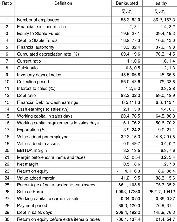
The inputs used in this study are presented in Table 1, consisting of 30 financial

ratios published by Coface1, which are available from Diane database.

(Table 1)

1 _{Coface is a credit risk provider in France that offers the Conan-Holder bankruptcy score, a score based}

Additionally we consider the ratio of Cash Earnings to Total Debt that Beaver (1966)

found to be the best single discriminator of bankruptcy, the 5 ratios used by Altman

(1968) in his Z-score model, which is a standard in bankruptcy, and the size, measured

by the logarithm of sales assuming that smaller firms may be more prone to bankruptcy

than larger firms.

For cases of negative equity, the return on equity could not be calculated and a

negative return of 150 percent was used instead.

As the number of healthier firms is higher than financially distressed, we

randomly excluded some healthier cases in order to get the following ratios of

bankrupted to healthy firms: 50/50, 36/64 and 28/72. It is known that lower ratios put

stronger bias towards healthy firms, deteriorating the generalization capabilities of the

network and increasing type II error.

Input selection

The number of inputs considered in this work is much larger than those used in

previous works, which usually employ no more than ten variables. Although some of

these inputs have small discriminatory capability in linear models, our neural network

method is capable of extracting information and improving the classification accuracy

without compromising generalization.

To select the inputs we used two procedures: elimination of highly correlated

ratios and ratios with small sensitivities, or with a wrong sign according to economic

analysis. We eliminated thirteen inputs (4, 6, 8, 9, 14, 16, 17, 22, 26, 27, 28, 29 and 30)

described in Table 1 and retained the remaining seventeen.

In many cases, some ratios present high variance from one year to another,

especially when firms are in financial distress. As a consequence, it is hard to predict

from a previous year, without overloading the neural network input with excessive

dimension, we decided to include one-year incremental absolute value of the following

ratios: Debt Ratio, Percentage of Value Added to Employees and the Margin Before

Extra Items and Taxes (or Ordinary Margin). Thus we end up with a complete set of 20

inputs.

All inputs were normalized in the usual way

k k k k x x

σ

µ

− = '

where µk is the mean and σk is the standard deviation of input element k.

6. Results

We tested several neural networks using from 5 to 20 hidden nodes. Although smaller

networks achieve slightly lower generalization errors, HLVQ-C performs better on a

hidden layer of a large size. Then, we chose a hidden layer of 15 neurons, a learning

rate of 0.1, and a momentum term of 0.25. For the HLVQ method we set β = 1.5.

Some firms in the database have a financial record that clearly contradicts their

actual financial status. For these evident cases, we decided to artificially invert their

output state. Companies with negative equity were always assigned to financial

distress category, independently of their originally category. Although this accounts for

less than 3% of bankruptcies some improvements were achieved on the training and

testing error.

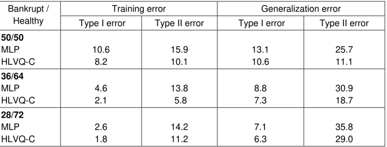
Table 2 shows the results obtained on balanced and unbalanced data sets for

the year 1999, approximately one year prior to the announcement of bankruptcy. The

training error is considerably smaller than the generalization error indicating that

training data is insufficient. As expected, type II error is higher than type I error since

indicates that it is not advisable to use unbalanced samples since type II error

increases considerably while type I error has only a slight improvement.

(Table 2)

In Table 3 we compare the weighted efficiency obtained by each of the four

methods. Balanced samples are more appropriate for all the classification methods

used while our method (HLVQ-C), clearly outperforms all others including discriminant

analysis and non-corrected MLP (traditional ANN) for all types of samples. Discriminant

analysis drops more in efficiency with unbalanced samples than neural networks.

HLVQ-C is the technique that shows lower loses.

(Table 3)

We repeated the analysis for 1998, which is approximately two years prior to

the bankruptcy announcement (Table 4). As expected all models show less predictive

power than one year prior to the financial distress announcement. Concerning the use

of unbalanced databases the same conclusions as 1999 apply.

(Table 4)

Again HLVQ-C performs much better than traditional neural networks – Table 5.

Moreover the difference between traditional neural networks and discriminant analysis

for balanced samples does not look significant.

(Table 5)

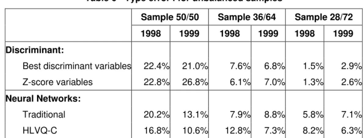
HLVQ-C also performs better for error I using balanced samples (Table 6). For

unbalanced samples, both neural networks have a better performance but present

worse type I errors. This indicates that they are less biased than discriminant analysis

(Table 6)

We also compared the efficiency of the Neural Network with the five ratios used in the

discriminant model (Debt Ratio, Logarithm of Sales, Value Added per Employee,

Cumulated Depreciation Ratio and Return on Assets), with a neural network of only 5

hidden nodes – Table 7. The generalization error, as expected, is slightly higher than

with the full 20 inputs. However, HLVQ-C was unable to correct efficiently these errors

since it does not have enough degrees of freedom.

(Table 7)

Sensitivity analysis from neural networks shows that the most significant ratios

for driving a company to financial distress (positive sensitivities) are: Debt Ratio,

Percentage of Value Added for Employees and one-year absolute variation of the Debt

Ratio. The most relevant ratios to characterize a healthy company (negative

sensitivities) are: Valued Added per Employee, Margin Before Extra Items and Taxes

and Cumulated Earnings to Assets.

7. Conclusions

We have applied neural networks to the problem of bankruptcy prediction using a new

technique to correct the generalization errors, called HLVQ-C. In contrast with

discriminant analysis and traditional neural networks, this technique allows the use of

larger set of inputs without compromising generalization.

A modified measure of classification efficiency used by Korobow and Stuhr

(1985) was introduced to evaluate the performance of the method. We found that

discriminant analysis and traditional MLP in detecting distressed companies both one

and two years prior to bankruptcy.

We also studied the effect of unbalanced samples and found that the best

performance is obtained with a balanced dataset containing the same number of

healthy and distressed companies. Unbalanced database should be avoided as type I

errors, which have higher costs for banks, may be too high.

These results could eventually be improved if we had the identification of the

industrial sector for each company, as some ratios may only be meaningful for some

sectors.

References

Altman, E.I., 1968. Financial Ratios, Discriminant Analysis and the Prediction of Corporate Bankruptcy. Journal of Finance, 23, 4, 589-609.

Altman, E.I., 1984a. A Further Empirical Investigation of the Bankruptcy Cost Question. Journal of Finance, September.

Altman, E.I., 1984b. The Success of Business Failure Prediction Models: An International Survey. Journal of Banking and Finance, 8, 171-198.

Altman, E.I., 1989. Measuring Corporate Bond Mortality and Performance. Journal of Finance, 44, 909-1022.

Altman, E.I., 1993. Corporate Financial Distress and Bankruptcy: A Complete Guide to

Predicting and Avoiding Distress and Profiting from Bankruptcy, 2nd Ed. John Wiley & Sons, New York.

Altman, E.I., Haldeman, R.G., Narayanan, P., 1977. Zeta Analysis. A new model to identify bankruptcy of corporations. Journal of Banking and Finance, 1, 29-54.

Altman, E.I., Marco, G., Varetto, F., 1994. Corporate Distress Diagnosis: Comparing using Linear Discriminant Analysis and Neural Networks (the Italian experience). Journal of Banking and Finance, 18, 505-529.

Amemiya, T., Powell, J. L., 1983. A comparison of the Logit Model and Normal Discriminant Analysis when Independent Variables are Binary, in: Karlin, Amemiya, Goodman (Eds), Studies in Econometric, Time Series, and Multivariate Statistics, 3-30, New-York.

Bardos, M., Zhu, W., 1997. Comparaison de l’Analyse Discriminante Linéaire et des Réseaux de Neurones, Application à la Détection de Défaillances d’Entreprises. Revue de Statistique Appliquée, XLV, 65-92.

Beaver, W.H., 1966. Financial Ratios as Predictors of Failures. Empirical Research in Accounting: Selected Studies, 1966, supplement to volume 5, Journal of Accounting Research, 71-102.

Bishop C. M., 1995. Neural Networks for Pattern Recognition. Oxford University Press, Oxford. Blum, M., 1974. Failing Company Discriminant Analysis. Journal of Accounting Research

Coats, P.K., Fant L.F., 1993. Recognising Financial Distress Patterns Using a Neural Network Tool. Financial Management (Autumn), 142-155.

Conan D., Holder, M., 1979. Variables explicatives de performance et contrôle de gestion dans les P. M. I. , Thèse d'Etat, CERG, Université Paris Dauphine.

Deakin, E.B., 1972. A Discriminant Analysis of Predictors of Financial Failure. Journal of Accounting Research (Spring), 167-179.

Edminster, R.O., 1972. An Empirical Test of Financial Ratio Analysis for Small Business Failure Prediction. Journal of Financial and Quantitative Analysis, (March), 1477-1493.

Huberty, C.J., 1984. Issues in the Use and Interpretation of Discriminant Analysis. Psychological Bulletin, Vol. 95, 156-171.

Jain, B., Nag B., 1997. Performance Evaluation of Neural Network Decision Models. Journal of Management Information Systems, Vol. 14, No. 2, (Fall), 201-216.

Klimasauskas, C.C., 1993, Applying Neural Networks, in: Trippi, R., Turban E., (Eds), Neural Networks in Finance and Investing, Probus Publishing Company, Chicago.

Korobow, L. , Stuhr, D., 1985. Performance of early warning models. Journal of Banking and Finance, 9, 267-273.

Lee, K.C., Han I., Known Y., 1996. Hybrid neural network models for bankruptcy predictions. Decision Support Systems 18, 63-72.

Lo, A.W., 1986, Logit versus Discriminant Analysis, A Specification Test and Application to Corporate Bankruptcies. Journal of Econometrics, 31, 151-178.

Martin, D., 1977. Early Warning of Bank Failure: A Logit Regression Approach. Journal of Banking and Finance, 1, 249-276.

McFaden, D., 1976. A Comment on Discriminant Analysis versus Logit Analysis. Annals of Economic and Social Measurement, 5, 511-524.

Michie, D., Spiegelhalter, D.J. and Taylor, C.C. 1994, Machine Learning, Neural and Statistical Classification. Ellis Horwood.

Neves, J.C, Andrade e Silva, J., 1998. Modelos de Análise do Risco de Incumprimento à Segurança Social. Centro de Estudos e Documentação Europeia/Fundação para a Ciência e Tecnologia, available at http://www.iseg.utl.pt/~jcneves/paper_relatorio_fct1.PDF

Ohlson, J.A., 1980. Financial Ratios and the Probability of Bankruptcy. Journal of Accounting Research, 18, 109-131.

Press, S.J. , Wilson, S., 1978. Choosing Between Logistic Regression and Discriminant Analysis. Journal of the American Statistical Association, 73, 699-705.

Shah, J.R., Murtaza, M. B., 2000. A Neural Network Based Clustering Procedure for Bankruptcy Prediction. American Business Review (June), 80-86.

Srinivasan, V., Kim, Y. H., 1987. Credit Granting: A comparative analysis of classifications procedures. The Journal of Finance, XLII, 665-683.

Stein, J., Ziegler W., 1984. The Prognosis and Surveillance of Risks from Commercial Credit Borrowers. Journal of Banking and Finance, 8, 249-268.

Taffler, R.J., 1982. Forecasting Company Failure in the U.K. Using Discriminant Analysis and Financial Ratio Data. Journal of Royal Statistical Society, (Series A), 342-358

Taffler R.J., 1984. Empirical Models for the Monitoring of UK Corporations. Journal of Banking and Finance, 8, 199-227.

Tan, K., 1991. Neural Network Models and the Prediction of Bank Bankruptcy, Omega International Journal of Management Science, Vol. 19, No. 5, 429-445.

Trippi, R.R., Turban, E., (eds), 1993. Neural Networks in Finance and Investing. Probus Publishing Company, Chicago.

Tsukuda, M., Baba S., 1994. Predicting Japanese Corporate Bankruptcy in Terms of Financial Data Using Neural Network. Computers Industrial Engineering, Vol. 27, N0. 1-4, 445-448. Udo, G., 1993. Neural Network Performance on the Bankruptcy Classification Problem.

Computers and Industrial Engineering, Vol. 25, No. 1-4, 377-380.

Varetto, F., 1998. Genetic Algorithms Applications in the Analysis of Insolvency Risk. Journal of Banking and Finance, 22, 1421-1439.

Vieira, A., Barradas N. P., 2003. A training algorithm for classification of high dimensional data. Neurocomputing, 50C, 461-472.

Vieira A., Castillo, P.A., Merelo, J.J., 2003. Comparison of HLVQ and GProp in the problem of bankruptcy prediction, in: J. Mira (Ed.) IWANN03 - International Workshop on Artificial Neural Networks, , LNCS 2687, Springer-Verlag pp. 655-662.

Table 1: Mean values and standard deviation of all indicators for bankrupt and healthy companies in the year of 1999

Bankrupted Healthy

Ratio Definition

i i

x

,

σ

x

_i

,

σ

_i

1 Number of employees 55.3, 82.0 86.2, 157.3

2 Financial equilibrium ratio 1.2, 2.1 1.4, 2.2

3 Equity to Stable Funds 19.9, 27.1 39.4, 19.3

4 Debt to Stable Funds 18.9, 77.3 10.8, 13.0

5 Financial autonomy 13.3, 32.4 37.6, 19.8

6 Cumulated depreciation rate (%) 69.4, 19.6 70.3, 14.5

7 Current ratio 1.1,0.6 1.6, 1.4

8 Quick ratio 0.8, 0.5 1.2, 1.3

9 Inventory days of sales 45.5, 66.8 45, 66.5

10 Collection period 56.0, 42.6 75, 32.8

11 Interest to sales (%) 1.2, 5.3 0.8, 2.8

12 Debt ratio 83.2, 32.3 59.0, 18.9

13 Financial Debt to Cash earnings 6.5,111.3 6.6, 119.1

14 Cash earnings to sales (%) 2.1, 13.0 4.4, 6.7

15 Working capital in sales days 20.4, 76.5 64.5, 86.3

16 Working capital requirements in sales days 16.1, 76.2 50.6, 70.2

17 Exportation (%) 3.9, 24.2 9.0, 21.1

18 Value added per employee 32.3, 15.3 44.6, 29.05

19 Value added to assets 0.5, 49.7 0.4, 0.2

20 EBITDA margin 3.3, 13.5 6.8, 7.6

21 Margin before extra items and taxes 0.3, 2.54 3.2, 3.4

22 Net margin 0.5, 18.6 1.2, 7.8

23 Return on equity -11.4, 116.3 8.9, 38.4

24 Value added margin 41.2, 19.5 38.3, 15.6

25 Percentage of value added to employees 86.1, 103.8 75.7, 35.2

26 Sales (kEuro) 9093, 17350 25217, 40412

27 Working capital to current assets 0.04, 0.53 0,36, 0.27

28 Payment period 89.0, 120.3 76.9, 31.4

29 Debt in sales days 208.4, 192.2 145.8, 76.3

Table 2: Results for a set of balanced and unbalanced data for the year of 1999. HLVQ-C means the output of the MLP are corrected by the method using HLVQ distances.

Training error Generalization error

Bankrupt /

Healthy _{Type I error Type II error Type I error Type II error}

50/50 MLP HLVQ-C 10.6 8.2 15.9 10.1 13.1 10.6 25.7 11.1 36/64 MLP HLVQ-C 4.6 2.1 13.8 5.8 8.8 7.3 30.9 18.7 28/72 MLP HLVQ-C 2.6 1.8 14.2 11.2 7.1 6.3 35.8 29.0

Table 3: Weighted efficiency for the year of 1999

Sample: 50/50 36/64 28/72

Discriminant:

Best discriminant variables 66.1% 60.2% 59.3%

Z-score variables 62.7% 52.1% 47.5%

Neural Networks:

MLP 71.4% 68.5% 65.0%

HLVQ-C 84.1% 78.9% 71.0%

Table 4: Weighted efficiency for the year of 1998

Sample: 50/50 36/64 28/72

Discriminant:

Best discriminant variables 66.4% 59.5% 47.3%

Z-score variables 61.1% 50.9% 32.0%

Neural Networks:

Traditional 67.7% 69.5% 60.1%

HLVQ-C 76.5% 74.3% 69.5%

Table 5 – Type error II for unbalanced samples

Sample 50/50 Sample 36/64 Sample 28/72

1998 1999 1998 1999 1998 1999

Discriminant:

Best discriminant variables 24.9% 26.4% 44.5% 44.6% 68.4% 51.5%

Z-score variables 31.6% 26.8% 57.1% 54.5% 83.2% 66.0%

Neural Networks:

Traditional 24.9% 25.7% 30.9% 30.9% 44.9% 35.8%

Table 6 - Type error I for unbalanced samples

Sample 50/50 Sample 36/64 Sample 28/72

1998 1999 1998 1999 1998 1999

Discriminant:

Best discriminant variables 22.4% 21.0% 7.6% 6.8% 1.5% 2.9%

Z-score variables 22.8% 26.8% 6.1% 7.0% 1.3% 2.6%

Neural Networks:

Traditional 20.2% 13.1% 7.9% 8.8% 5.8% 7.1%

HLVQ-C 16.8% 10.6% 12.8% 7.3% 8.2% 6.3%

Table 7: Neural Networks trained with the five inputs chosen by the discriminant analysis, in the year 1999 using the balanced database.

Training error Generalization error

Type I error Type II error Type I error Type II error MLP

HLVQ-C

15.6 10.5

20.1 14.3

17.1 14.8