CliPick: Project database of Pan-European simulated climate data for default model use

AGFORWARD (Grant Agreement N° 613520) is co-funded by the European Commission, Directorate General for Research & Innovation, within the 7th Framework Programme of RTD. The views and opinions expressed in this report

CliPick: Project Database of Pan-European

Simulated Climate Data for Default Model Use

Work-package 6: Field- and Farm-scale Evaluation of Innovations

Milestone Milestone 26 (6.1): CliPick: Project Database of Pan-European Simulated Climate Data for Default Model Use

Date of report 20 June 2014; updated 10 October 2015 Authors João H.N. Palma

Contact joaopalma@isa.ulisboa.pt

Reviewed Anil Graves and Paul J. Burgess

Contents

1 Context ... 2

2 Online tool (Front-end) ... 3

3 Source of data, storage and extraction process (Back-End) ... 5

4 Accessibility ... 13

5 Data quality ... 18

6 Acknowledgments ... 20

7 References ... 20

Annex A. NetCDF Files stored in ISA server, providing data for CliPick ... 21

1

Context

The aim of the AGFORWARD project (January 2014-December 2017) is to promote agroforestry practices in Europe that will advance sustainable rural development. Within the project there are four objectives:

1. to understand the context and extent of agroforestry in Europe,

2. to identify, develop and field-test innovations to improve the benefits and viability of agroforestry systems in Europe,

3. to evaluate innovative agroforestry designs and practices for locations where agroforestry is currently not-practised or is declining, and quantify the opportunities for uptake at a field and farm-scale and at a landscape-scale, and

4. to promote the wider adoption of appropriate agroforestry systems in Europe through policy development and dissemination.

The third objective is addressed partly by work-package 6 which focused on the field- and farm-scale evaluation of innovations. During the later stages of the AGFORWARD project, agroforestry modelling will be used to evaluate different scenarios and case studies across Europe. The agroforestry models being used on the project are Yield-SAFE (van der Werf et al., 2007) and Hi-SAFE (Talbot, 2011). Both require daily weather data as inputs and this report covers development of Milestone 26 (6.1) for work-package 6, which is to develop a “project database of pan-European simulated climate data for default model usage”.

The database called CliPick takes the form of an internet-based on-line platform. This means that it can be accessed not only by modellers in the AGFORWARD consortium but also other users in the scientific community needing climate data (including climate change) for modelling exercises. The output of this milestone was described at the 2nd European Agroforestry Conference (Palma, 2014)1. A poster of the tool delivered with Milestone 26 (6.1) and is available at: http://hdl.handle.net/10400.5/6830

In this update in October 2015, the CliPick tool now uses datasets from the 5th Assessment Report of the IPCC. In addition, the tool has been improved in terms of speed of retrieval to improve efficiency in the usage of web-based version of the Yield-SAFE model.

1

2

Online tool (Front-end)

The milestone output can be viewed as an online web-based tool called: “CliPick – Climate Change Web Picker” (Figure 1). Since June 2014, it has been available at the following web address: http://home.isa.utl.pt/~joaopalma/projects/agforward/clipick/

Figure 1. Front-end of CliPick, the climate change web picker 2.1 Principles

The CliPick tool aims to deliver user-friendly access to the climate database for general public use delivering the data in a format suitable for the AGFORWARD models (Yield-SAFE and Hi-SAFE). The tool also aims to provide data of acceptable quality to enable comparisons between current and future climates to observe impacts of climate change on agroforestry systems. Finally, the tool aims to allow access to programming interfaces to allow direct usage in modelling tools. This will extend its use and usefulness.

2.2 Target end-users

It is initially anticipated that the main users of the tool will be researchers with modelling tasks from work-package 6 within the AGFORWARD project. However the tool has been made available on the Web so that it can be used by any member of the scientific community needing climate data for modelling purposes. Currently, the tool supports output formats required by Yield-SAFE and Hi-SAFE agroforestry models but other formats could be added.

2.3 Steps to retrieve data

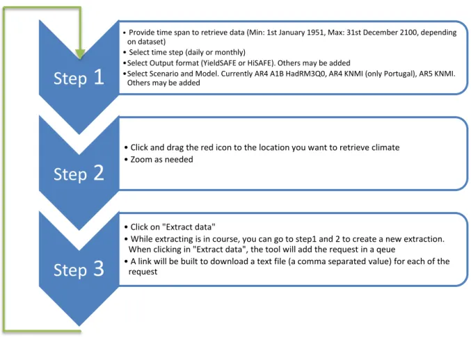
Figure 2. Steps to retrieve data from CliPick. The result will be the download of a comma separated value text file.

In Step 1, the earliest starting date possible is 1 January 1951 and the latest possible end date is the 31 December 2100. However this will depend on the dataset selected. For example, the IPCC Assessment Report 5 datasets are available for separated time frames (1951-2005, 1981-2010 and 2006-2010). These limits are consistent with the limits of the source datasets (see Section 3.1). The source data are provided at a daily time-step. Thus, daily data can be extracted directly from the source data, whilst monthly data must be calculated accordingly, but also available to download by selecting the “time step” options.

In Step 2, the user selects a location for which the data must be retrieved. The data are extracted for the nearest grid point (25 km and 11 km resolution in AR4 and AR5 respectively) using the icon as in Figure 1. It is important the user understands that this location, in AR4 datasets, is within a 10-15 km radius of the nearest grid point and will likely provide the same data. With AR5 datasets the resolution increased and this radius decreased to about 5 km. It is also important to understand that, because of the resolution of the data, locations near particular geomorphological structures (e.g. mountains, coastline) may retrieve data which is not representative of a location (see section 5).

A particular feature of Step 3 is the ability to queue data extraction. Each of the user requirements for data in Steps 1 and 2 will build a URL that will be sent to the server. When a request is made, it will not be overwritten by a subsequent request. All requests are performed on a “first come, first

Step

1

• Provide time span to retrieve data (Min: 1st January 1951, Max: 31st December 2100, depending on dataset)

• Select time step (daily or monthly)

•Select Output format (YieldSAFE or HiSAFE). Others may be added

•Select Scenario and Model. Currently AR4 A1B HadRM3Q0, AR4 KNMI (only Portugal), AR5 KNMI. Others may be added

Step

2

• Click and drag the red icon to the location you want to retrieve climate • Zoom as needed

Step

3

• Click on "Extract data"

• While extracting is in course, you can go to step1 and 2 to create a new extraction. When clicking in "Extract data", the tool will add the request in a qeue

• A link will be built to download a text file (a comma separated value) for each of the request

serve” basis. If the server is already busy with requests, new requests will have to wait. The delay will depend on how busy the server is.

2.4 Additional Information

The tool supplies additional information in the central section, near the Step 2 tab. The tool will be updated during (and after) the project if improvements are required.

“Instructions” tab: the steps from Figure 2 have been added to this tabbed section, and include a tutorial video that demonstrates how to retrieve the data.

“Info” tab: this section provides the context for the tool. It will be updated accordingly, and will also include a link to this milestone report and AGFORWARD.

“AQs” tab: AQs stands for “Asked Questions” and aims to provide a forum of questions and answers allowing sharing of thoughts and ideas on the use of the tool and data.

“Who’s using this” tab: this tab provides a counter on users accessing the tool, allowing a monitoring of the tool use for reference. No personal data is collected.

3

Source of data, storage and extraction process (Back-End)

The ENSEMBLES datasets repository (http://www.ensembles-eu.org/) as well as CORDEX (www.cordex.org) were used to provide the source data for CliPick. The advantage of working with these datasets is that the agroforestry modelling projections will use climate data that draw on the datasets sent to the International Panel on Climate Change (IPCC) by National Agencies (see Annexes A and B).

3.2 Climate change scenarios brief context 3.2.1 IPCC Assessment Report 4

The IPCC climate change scenarios (AR4) relate to different scenarios of greenhouse gas emissions in the future based on global human activity and development. The scenarios are called: A1 (A1FI, A1B, A1T), A2, B1 and B2, and these are shown in Figure 3. An excerpt from the IPCC (2000) describing the climate change scenarios is provided for information:

“By 2100 the world will have changed in ways that are difficult to imagine – as difficult as it would have been at the end of the 19th century to imagine the changes of the 100 years since. Each storyline assumes a distinctly different direction for future developments, such that the four storylines differ in increasingly irreversible ways. Together they describe divergent futures that encompass a significant portion of the underlying uncertainties in the main driving forces. They cover a wide range of key “future” characteristics such as demographic change, economic development, and technological change. For this reason, their plausibility or feasibility should not be considered solely on the basis of an extrapolation of current economic, technological, and social trends.

• The A1 storyline and scenario family describes a future world of very rapid economic growth, global population that peaks in mid-century and declines thereafter, and the rapid introduction of new and more efficient technologies. Major underlying themes are convergence among regions, capacity building, and increased cultural and social interactions, with a substantial reduction in regional differences in per capita income. The A1 scenario family develops into three groups that describe alternative directions of technological change in the energy system. The three A1 groups are distinguished by their technological emphasis: fossil intensive (A1FI), non-fossil energy sources (A1T), or a balance across all sources (A1B).

• The A2 storyline and scenario family describes a very heterogeneous world. The underlying theme is self-reliance and preservation of local identities. Fertility patterns across regions converge very slowly, which results in continuously increasing global population. Economic development is primarily regionally oriented and per capita economic growth and technological change are more fragmented and slower than in other storylines.

• The B1 storyline and scenario family describes a convergent world with the same global population that peaks in mid-century and declines thereafter, as in the A1 storyline, but with rapid changes in economic structures toward a service and information economy, with reductions in material intensity, and the introduction of clean and resource-efficient technologies. The emphasis is on global solutions to economic, social, and environmental sustainability, including improved equity, but without additional climate initiatives.

• The B2 storyline and scenario family describes a world in which the emphasis is on local solutions to economic, social, and environmental sustainability. It is a world with continuously increasing global population at a rate lower than A2, intermediate levels of economic development, and less rapid and more diverse technological change than in the B1 and A1 storylines. While the scenario is also oriented toward environmental protection and social equity, it focuses on local and regional levels.”

Figure 3. IPCC AR4 carbon emission predictions related to scenarios nomenclature (Source: IPCC (2000)

Research studies usually select a particular scenario, often a moderate scenario where society evolves through a balanced use of energy from fossil and non-fossil fuel (Scenario A1B). Following the same approach, CliPick provides data for scenario A1B: “balance across all sources”.

3.2.2 IPCC Assessment Report 5

In IPCC assessment report 5, the scenarios have different taxonomy, the so called Representative Concentrations Pathways (RCP), where CO2eq concentration in the atmosphere determines the scenario name (Figure 4).

A)

B)

Figure 4. A) Definition of CO2eq concentration categories in IPCC 5th Assessment Report, adapted from Clarke et al. (2014); B) Global greenhouse gas emissions for the different RCP scenarios, adapted from IPCC (2014).

Dufresne et al (2013) provides us a comparison between AR4 and AR5 scenarios, where we can conclude that scenario A1B, from the previous IPCC assessment report, can be positioned near RCP6, in between RCP4.5 and RCP8.5 (Figure 5). CliPick adopted an optimistic scenario, the RCP4.5, and a pessimistic scenario, the RCP8.5.

Figure 5. Comparison of temperature anomaly and radiative forcing between AR4 (SRES) and AR5 (RCP) scenarios. Adapted from Dufresne et al. (2013)

3.2.3 Climate models

Climate models are developed by different research groups. The models try to project how climate will be under each scenario. Each particular research group has its own methods and algorithms and this raises the question on “which model to use”. Amongst the available climate models in AR4 there were the ECHAM family, and the ARPEGE, MIROC, CGCM, BCM, Hadley Center Climate Model (HADCM), HADRM, and IPSLc models. These may naturally expand in future. With the undergoing CORDEX (COordinated Regional climate Downscaling Experiment - http://www.cordex.org/), the numerous models are listed in the website.

HADCM and RACMO was chosen for CliPick because work by Soares et al. (2012) found a good fit for these models for the Portuguese context, furthermore these models were generally found to fit other regions in Europe well (Soares et al., 2012). Therefore CliPick provides data from scenario A1B as projected by the Hadley Center Climate Model and two scenarios, RCP4.5 and RCP 8.5, developed by the Royal Netherlands Meteorological Institute (KNMI).

3.2.4 Resolution and climate variables

The Global Climate Model (GCM) provides a resolution of about 350 km. The ENSEMBLES project down-scaled this data to a Regional Climate Model (RCM), providing a 25 km grid. The CORDEX project downscaled the resolution to about 11 km. The output time scale varies from 6 hours to monthly data. CliPick uses the daily datasets because YieldSAFE and HI-SAFE need this temporal scale.

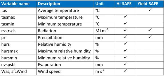
Numerous climate variables are simulated in RCM. However, only a small number of variables are needed for Yield-SAFE and Hi-SAFE. These are: average, minimum, and maximum temperature, radiation, precipitation, average, minimum and maximum relative humidity, evaporation and wind speed (Table 1).

Table 1. Climate variables being accessed in CliPick and use with HI-SAFE and Yield-SAFE

Variable name Description Unit Hi-SAFE Yield-SAFE

tas Average temperature °C 

tasmax Maximum temperature °C 

tasmin Minimum temperature °C 

rss,rsds Radiation MJ m-2  

pr Precipitation mm  

hurs Relative humidity % 

hursmax Maximum relative humidity %  hursmin Minimum relative humidity % 

evspsbl Evaporation mm 

Wss, sfcWind Wind speed m s-1 

3.2.5 Data format

The most common format used by climate modelers to exchange data is the network common data format (NETCDF) which is a binary file containing array-oriented scientific data to ease data exchange between climate modelers. Another common characteristic of climate datasets is their large size because the work is usually done at global scale. Even with binary formats, the large areas (e.g. European scale, including oceans) and the time span (often 100 years into the future) delivers so much data that it needs to be mined since modelling often requires less data.

The initial strategic option selected in CliPick was to directly access the NETCDF files. This would enable inclusion of other scenarios and models with minimal programming effort in terms of future data access. If CliPick would be required for different scenarios or models, a direct copy of NETCDF files from the EMSEMBLES repository to the server could have been made. All the extraction algorithms were prepared to extract NETCDF files using the same structure and will be used to direct the data to the online platform.

ENSEMBLES provides individual files for one decade of a particular climate variable. This means that there are 15 files for each of the 10 variables listed in Table 1. Each file is about 450 MB in size, which means there are approximately 67.5 GB of stored data in total.

The list of the NETCDF files present in the server are listed in Annex A. The nomenclature of the files is from the ENSEMBLES project.

[UPDATE Oct 2015] To increase performance of Clipick, in particular the speed access, the files have been preprocessed and the netcdf process is by-passed.

3.3 Current and future climate comparisons

The ENSEMBLES datasets generation method consists in calibrating a climate model with observed data (e.g. 1960-1990). Once the climate model is calibrated, a simulation starts on the 1st of January 1951, simulating climate data until 1990 where simulated data should broadly reproduce the trend of observed data. Then, from 1990 onwards, the drivers of climate change scenarios are introduced in the simulation modelling.

The CORDEX datasets are divided in four parts, named historical, evaluation rcp45 and rcp85. The historical dataset is the representation of the observed historical data (1951-2005). The evaluation dataset is a simulation of the observed data ranging from 1981 to 2010. The rcp45 and rcp85 are projections with climate change scenarios and range from 2006 to 2010. It is suggested, for comparing current vs future climate, that the datasets used for comparison are the evaluation for current climate while rcp45 and rcp85 are used for future representations.

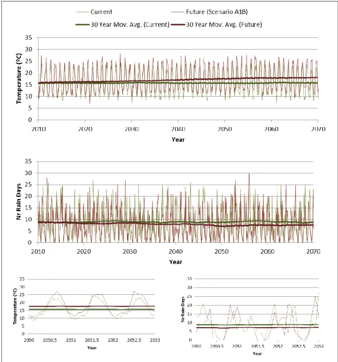
For the modelling of agroforestry systems, or any other model requiring climate data, in order to assess projections with current climate, the projections should be from 1960 until 1990. If more than 30 years is needed, the same climate should be added as blocks of 30 years with the same data. An example of comparison is given in

Figure 6, where 30 year blocks of climate from 1960-1990 are repeated to future while the future climate is provided by the dates from the dataset.

Figure 6. Example of comparison between current and future climate between 2010 and 2070 and a focus between 2050-2053, for mean annual temperature and number of rain days near Coruche, south Portugal

3.4 Extraction process

The 150 NETCDF files are stored in the server and algorithms were developed to access the datasets and provide data that that could be read in a format other models (or humans!) could read.

The main goal was to produce a file with a format that could be read by most of the people: a text file with comma separated values (csv).

The front-end is the means to collect information from the user. This visual interface was made with application programming interface (API) of Google Maps, the JavaScript libraries of DOJO 1.7.5 (http://dojotoolkit.org/) and JQuery 1.10.3 (http://jquery.com/).

To collect that user information and organize it to produce requests for the NETCDF files, the server side programming languages PHP (www.php.net) and Python (www.python.org) were used. To combine both server and client-side languages, the programming technique of Asynchronous JavaScript and XML (AJAX) was used.

The following steps are used in CliPick (resume in Figure 7):

1. User inputs are collected and build a “Climate Request”, a URL created in javascript, and sent to the server via AJAX

2. A PHP algorithm identifies in the request which NETCDF files are going to be accessed

3. The PHP algorithm creates a pool of HTTP requests for a Python algorithm that is executed in parallel

4. The Python algorithm accesses one file at a time (1 decade of 1 variable) and sends the response back to the PHP algorithm

5. Another PHP algorithm collects the responses and organizes the information to deliver to the front-end via AJAX

6. The list of climate variables and time frame are filtered from the preprocessed files 7. The front-end creates a link to download the text data

8. [Update Oct 2015] Steps 2, 3, 4 and 5 are now by passed as these are preprocessed to improve speed performance.

The extraction of data does not have to follow the front-end interface request. The server can be accessed directly an alternative ways to implement it are described in section 4-Accessibility, page 13.

A)

B)

Figure 7. Fluxogram for the climate data extraction in CliPick: A) version pre Oct 2015 and B) Oct 2015 onwards, improving access speed.

4

Accessibility

The easiest way to access CliPick data is the online user-friendly front-end interface providing a link to download the data. However the architecture of CliPick was built to deliver data in different ways. Another option to the online user-friendly tool is to programmatically access the data. Any programming language can access CliPick as long as it provides HTTP Requests routines (see Sections 4.1 and 4.2).

The programmatic access to datasets was tested with success and the performance of the server observed. The server also hosts other websites for ISA, and rigorous testing using a loop in the python algorithm below (Box 1), was executed, and the response observed on the websites being served by the same machine.

The server behaved with a queuing strategy, where the processor was occupied with no more than a proportion of the CliPick requests, whilst the remaining resources were used for serving the other websites hosted. These seemed to behave normally.

The “first come, first served” strategy may slow down the access to the data when many users (including those accessing it programmatically) are simultaneously accessing the tool. Further improvements are being made to address this issue so that the access strategy can include a “smart request override” that will access data from a different source, dependent on intensity of CliPick

usage. In other words, accessing the same data twice (same location) will: 1) release the server from data load, and; 2) speed up response speed to the requests.

4.1 Example of a python script to extract data from clipick

The architecture of CliPick was built to deliver data in different ways. Another option is to programmatically access the data. Any programming language can access CliPick as long as it provides HTTP request routines.

Python is currently a programming trend. This language is open source and its use has been growing rapidly in the last years. To run this script you just need: 1) to install a python interpreter (www.python.org ); 2) a simple text editor (e.g. http://notepad-plus-plus.org/), and; 3) to save your files with an extension “.py”. Box 1 shows an example of python script for retrieving daily data, and exporting the results to a text file.

Box 1. Code example for a Python implementation to create a text file of climate data through access Below an example in Python retrieving daily data, exporting results to a text file.

#!/usr/bin/env python # coding: UTF-8 -*-# enable debugging import cgitb cgitb.enable() import csv import StringIO import urllib2 import urllib import time

# Make this piece of text working as a program

'''

Open notepad or a similar simple text editor Copy-paste this boxed text to the opened document Save it as a file named myfilename.py

If you have not installed python, download it and install from www.python.org After installation, browse your myfilename.py and double click it

It should open a “black screen” for about 10 seconds and then it closes. A file should be created called ClipickExportedData.csv in the same directory play around with the section “CONTROL VARIABLES OF THIS ALGORTIHM“ to retrieve different date ranges (expect more or less than ten seconds. More daily data will increase the retrieval time.

'''

# Needed daily DATA: # Column 0: Year # Column 1: Month # Column 2: Day

# Column 3: Average temperature (degrees C) # Column 3: Radiation (MJ / sq meter) # Column 3: Precipitation (mm)

#CONTROL VARIABLES OF THIS ALGORTIHM:

you can explore other options here. you can try to create a loop if you need several locations or several

'''

#

Longitude = -8.335343513 Latitude = 39.2816836

StartYear = 2000 # Min=1951, Max=2100 StartMonth = 1 StartDay = 1 EndYear = 2003 EndMonth = 12 EndDay = 31 IPCCAssessmentReport = 4 # either 4 or 5

#the file to export the output:

outFileName = 'ClipickExportedData.csv' # tip you can build the name of the file to be according to the dates extracted

outFileHandle = open(outFileName, 'w')

start_time = time.time() # this is facultative, just to calculate timming of retrieval

# Build the HTTP REQUEST pars = {}

pars['lat'] = Latitude pars['lon'] = Longitude

pars['fmt'] = 'csv' # either csv, htmltable pars['tspan'] = 'd'# d=daily; m =monthly pars['sd'] = StartDay #'01'

pars['sm'] = StartMonth #'01' pars['sy'] = StartYear pars['ed'] = EndDay pars['em'] = EndMonth pars['ey'] = EndYear

pars['dts'] = 'METO-HC_HadRM3Q0_A1B_HadCM3Q0_DM_25km' # if ar=4 use METO-HC_HadRM3Q0_A1B_HadCM3Q0_DM_25km. If ar=5 use either knmihistorical,

knmievaluation, knmircp45, knmircp85. Beware of dates for extraction pars['ar'] = 4 # either 4 or 5

pars['mod'] = "hisafe" # either yieldsafe or hisafe url =

'http://home.isa.utl.pt/~joaopalma/projects/agforward/clipick/climaterequest_fast. php'

url_pars = urllib.urlencode(pars) full_url = url + '?' + url_pars print "Request made to " + full_url response = urllib2.urlopen(full_url) the_page = response.read()

f = StringIO.StringIO(the_page) reader = csv.reader(f, delimiter=',')

# CEATE AN ARRAY FROM THE REQUESTED CSV OUTPUT result=[]

for row in reader: result.append(row)

# WRITE IT DOWN IN THE OUTPUT FILE

'''

the daily output comes as

yieldsafe : Day, Month, Year, tas, rss, pr

hisafe : Day, Month, Year, tasmax,tasmin,hursmax,hursmin,rss,pr,wss

in AR5 datasets, there are no min and max relative humidity (at the time of this deliverable).

therefore, at the moment, hisafe format for AR5 are as follows:

hisafe: : Day, Month, Year, tasmax,tasmin,hurs,evspsbl,rsds,pr,sfcWind

Currently Valid variables are (nomenclature as ENSEMBLES, and CORDEX project): "pr" : precipitation

"tas" : Average Temperature "tasmin" : Minimum Temperature "tasmax" : Maximum temperature "rss" : Radiation

"evspsbl": Evaporation "hurs" : Relative Humidity

"hursmax": Maximum Relative humidity "hursmin": Minimum Relative humidity "wss" : Wind Speed (ensembles) "sfcWind": Wind Speed (coredex) '''

# WRITE THE RESULTS IN THE FILE AND CLOSE IT

print "Output is being written in " + outFileName for i in result: outFileHandle.write(",".join(i) + "\n") outFileHandle.flush() outFileHandle.close() #Facultative... end_time = time.time()

print "Processed in " + str(round(end_time - start_time,0)) + " seconds"

print "Output stored in " + outFileName print "done"

4.2 Example of Excel acquiring data from CliPick

Probably the most commonly used spreadsheet is Microsoft Excel. This spreadsheet can also access data directly from the web. Additionally, Visual Basic for Applications can provide a useful tool for automating the process, for example for importing data to the Microsoft Excel version of Yield-SAFE (see Graves et al., 2007, 2010).

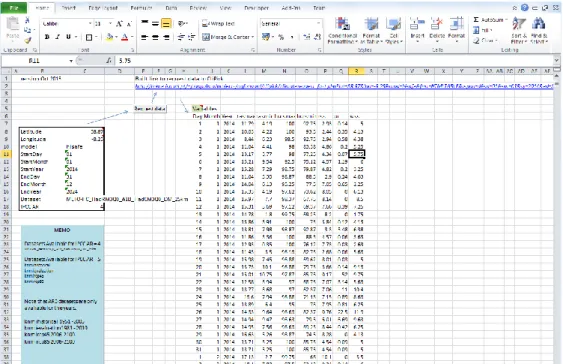
Below is an example of Microsoft Excel being used to collect data from CliPick (Figure 8). Using the geographical and other parameter inputs in the black box in Figure 8, a link is automatically built in Cell E2 (see footnote2 for its contents). The “Request data” button triggers the code shown in Box 2 that creates the request, reads the response from the server and pastes the information into data array starting at cell I6.

Figure 8. Example of a Microsoft file for extracting data from CliPick. The button activates the code from Box 2

Box 2. Visual Basic for Applications code for a request to CliPick, storing the result in Cell I6 Sub RequestClimate2Clipick()

'

' RequestClimate2Clipick Macro '

Dim URLString As String

URLString = "URL;" & Range("E2").Value

With ActiveSheet.QueryTables.Add(Connection:= _ URLString, _ Destination:=Range("$I$6")) .Name = "ClimateRequest" .FieldNames = True .RowNumbers = False .FillAdjacentFormulas = False .PreserveFormatting = True 2 Cell E2 contents: =CONCATENATE("http://home.isa.utl.pt/~joaopalma/projects/agforward/clipick/climaterequest_fast.php?lat= ",C8,"&lon=",C9,"&mod=",C10,"&fmt=HTMLTABLE&tspan=d&sd=",C11,"&sm=",C12,"&sy=",C13,"&ed=",C14," &em=",C15,"&ey=",C16,"&dts=",C17,"&ar=",C18)

.RefreshOnFileOpen = False .BackgroundQuery = True .RefreshStyle = xlOverwriteCells .SavePassword = False .SaveData = True .AdjustColumnWidth = True .RefreshPeriod = 0 .WebSelectionType = xlEntirePage .WebFormatting = xlWebFormattingNone .WebPreFormattedTextToColumns = True .WebConsecutiveDelimitersAsOne = True .WebSingleBlockTextImport = False .WebDisableDateRecognition = False .WebDisableRedirections = False .Refresh BackgroundQuery:=False End With

End Sub

5

Data quality

The quality of the data is strictly related to the ENSEMBLES and CORDEX projects’ output data. CliPick does not model climate data but extracts data from previously generated datasets. Therefore, CliPick relies on the robustness of the ENSEMBLES and CORDEX methodology.

The data should be used for model projections rather for model calibrations because the dataset is composed of simulated data. However work is currently being done to assess the use of this data for calibration and validation of forest growth models

To calibrate trees and crops, observed data should be used. This should either be collected by the different partners in the consortium for experimental plots, or from national datasets. There are also other sources of daily climate data for European countries, such as the European Climate Assessment & Dataset (www.eca.knmi.nl) that could be used to provide observed data for calibration procedures.

5.1 Feedback

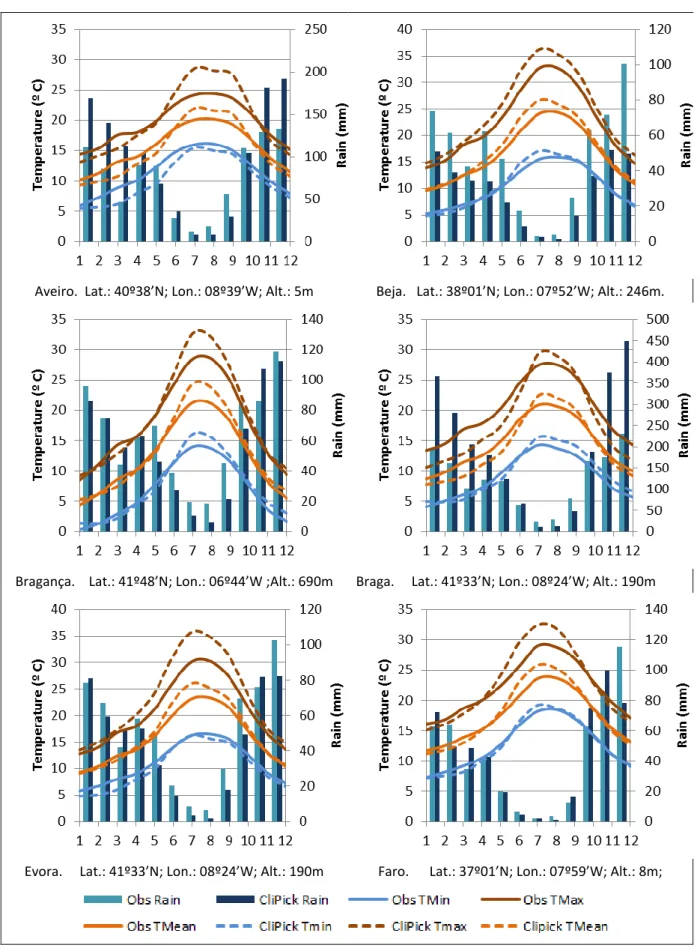
During the developing phase of the tool an email was sent to AGFORWARD consortium, asking for the tool to be tested to verify if the CliPick climate data made sense for known locations, either at places where local climate data was available (e.g. experimental sites) or where it was known from national climate databases collecting historical climate data (e.g. 1960-1990). The feedback varied from simple emails stating that the values were making sense, to more detailed analysis. In general, good feedback was provided for Germany, Denmark, UK, France, Spain (Extremadura), The Netherlands, and Italy. A more detailed overview was provided for Portugal (Figure 9).

5.2 Further quality assessments

During use of the data, a deeper analysis of the data is planned. The online tool will be updated when needed, in response to new developments during the project, and usage of the tool.

Aveiro. Lat.: 40º38’N; Lon.: 08º39’W; Alt.: 5m Beja. Lat.: 38º01’N; Lon.: 07º52’W; Alt.: 246m.

Bragança. Lat.: 41º48’N; Lon.: 06º44’W ;Alt.: 690m Braga. Lat.: 41º33’N; Lon.: 08º24’W; Alt.: 190m

Evora. Lat.: 41º33’N; Lon.: 08º24’W; Alt.: 190m Faro. Lat.: 37º01’N; Lon.: 07º59’W; Alt.: 8m;

Figure 9. Comparison of CliPick monthly means 2000) and Portuguese climate means (1970-2000) for rainfall and minimum and maximum temperatures (Source: www.ipma.pt)

6

Acknowledgments

The AGFORWARD project (Grant Agreement N° 613520) is co-funded by the European Commission, Directorate General for Research & Innovation, within the 7th Framework Programme of RTD, Theme 2 - Biotechnologies, Agriculture & Food. The views and opinions expressed in this report are purely those of the writers and may not in any circumstances be regarded as stating an official position of the European Commission.

This tool had the support of the IT team of ISA, in particular the systems administrator Tiago Picado, especially on identifying the best solutions of implementation and evaluating the “stress tests” on the server. Additionally, we thank Mário David and all the support of the Laboratório de Investigação de Partículas (www.lip.pt) who facilitated the use of the European Grid Infrastructure (www.egi.eu) through the usage of the High Performance Computing (HPC) machines under the Infraestrutura Nacional de Computação Distribuída. The support is gratefully acknowledged.

7

References

Clarke L., Jiang, K., Akimoto K., Babiker M., Blanford G., Fisher-Vanden K., Hourcade J.-C., Krey V., Kriegler E., Löschel A., McCollum D., Paltsev S., Rose S., Shukla P. R., Tavoni M., van der Zwaan B. C. C., van Vuuren D.P. (2014). Assessing Transformation Pathways. In: Climate Change 2014: Mitigation of Climate Change. Contribution of Working Group III to the Fifth Assessment Report of the Intergovernmental Panel on Climate Change (Eds: Edenhofer, O., Pichs-Madruga R., Sokona Y., Farahani E., Kadner S., Seyboth K., Adler A., Baum I., Brunner S., Eickemeier P., Kriemann B., Savolainen J., Schlömer S., von Stechow C., Zwickel T., Minx J.C.). Cambridge University Press, Cambridge, United Kingdom and New York, NY, USA.

Dufresne, J.L., Foujols, M., Denvil, S., Caubel, a., Marti, O., Aumont, O., Balkanski, Y., Bekki, S., Bellenger, H., Benshila, R., Bony, S., Bopp, L., Braconnot, P., Brockmann, P., Cadule, P., Cheruy, F., Codron, F., Cozic, a., Cugnet, D., de Noblet, N., Duvel, J.P., Ethé, C., Fairhead, L., Fichefet, T., Flavoni, S., Friedlingstein, P., Grandpeix, J.Y., Guez, L., Guilyardi, E., Hauglustaine, D., Hourdin, F., Idelkadi, a., Ghattas, J., Joussaume, S., Kageyama, M., Krinner, G., Labetoulle, S., Lahellec, a., Lefebvre, M.P., Lefevre, F., Levy, C., Li, Z.X., Lloyd, J., Lott, F., Madec, G., Mancip, M., Marchand, M., Masson, S., Meurdesoif, Y., Mignot, J., Musat, I., Parouty, S., Polcher, J., Rio, C., Schulz, M., Swingedouw, D., Szopa, S., Talandier, C., Terray, P., Viovy, N., Vuichard, N. (2013). Climate change projections using the IPSL-CM5 Earth System Model: From CMIP3 to CMIP5, Climate Dynamics. doi:10.1007/s00382-012-1636-1

Graves, A.R., Burgess, P.J., Palma, J.H.N., Herzog, F., Moreno, G., Bertomeu, M., Dupraz, C., Liagre, F., Keesman, K., van der Werf, W., de Nooy, A.K., van den Briel, J.P. (2007). Development and application of bio-economic modelling to compare silvoarable, arable, and forestry systems in three European countries. Ecol. Eng. 29, 434–449. doi:DOI 10.1016/j.ecoleng.2006.09.018 Graves, A.R., Burgess, P.J., Palma, J., Keesman, K.J., van der Werf, W., Dupraz, C., van Keulen, H.,

Herzog, F., Mayus, M. (2010). Implementation and calibration of the parameter-sparse Yield-SAFE model to predict production and land equivalent ratio in mixed tree and crop systems under two contrasting production situations in Europe. Ecol. Modell. 221, 1744–1756. doi:10.1016/j.ecolmodel.2010.03.008

IPCC (2014). Climate Change 2014 Synthesis Report Summary Chapter for Policymakers. Ipcc 31. doi:10.1017/CBO9781107415324

IPCC (2000). IPCC special report - Emission Scenarios - Summary for Policymakers. Intergovernmental Panel on Climate Change. https://www.ipcc.ch/pdf/special-reports/spm/sres-en.pdf

Palma, J.H.N. (2014). CliPick–Climate Change Web Picker. Bridging climate and biological modeling scientific communities. 2nd Eur. Agrofor. Conf. - Integr. Sci. Policy to Promot. Agrofor. Pract. Soares, P.M.M., Cardoso, R.M., Miranda, P.M. a, de Medeiros, J., Belo-Pereira, M., Espirito-Santo, F.,

(2012). WRF high resolution dynamical downscaling of ERA-Interim for Portugal. Clim. Dyn. 39, 2497–2522. doi:10.1007/s00382-012-1315-2

Talbot, G. (2011). L’intégration spatiale et temporelle des compétitions pour l'eau et la lumière dans un système agroforestiers noyers-céréales permet-elle d'en comprendre la productivité? INRA, Umr Syst. Université de Montpellier, Montpellier.

van der Werf, W., Keesman, K., Burgess, P., Graves, A., Pilbeam, D., Incoll, L.D., Metselaar, K., Mayus, M., Stappers, R., van Keulen, H., Palma, J., Dupraz, C., 2007. Yield-SAFE: A parameter-sparse, process-based dynamic model for predicting resource capture, growth, and production in agroforestry systems. Ecol. Eng. 29, 419–433. doi:10.1016/j.ecoleng.2006.09.017

Annex A. NetCDF Files stored in ISA server, providing data for CliPick

The names of the files were kept identical to the nomenclature provided by the ENSEMBLES (AR4) and CORDEX (AR5) project. The “.nc” extension denotes a “NETDCF” file format. Each file has a size of about 450 MB. The total sum of files has a about 250 GB.

File Nr File Name

IPCC AR4 1 METO-HC_HadRM3Q0_A1B_HadCM3Q0_DM_25km_1951-1960_tas.nc 2 METO-HC_HadRM3Q0_A1B_HadCM3Q0_DM_25km_1951-1960_tasmax.nc 3 METO-HC_HadRM3Q0_A1B_HadCM3Q0_DM_25km_1951-1960_tasmin.nc 4 METO-HC_HadRM3Q0_A1B_HadCM3Q0_DM_25km_1951-1960_rss.nc 5 METO-HC_HadRM3Q0_A1B_HadCM3Q0_DM_25km_1951-1960_pr.nc 6 METO-HC_HadRM3Q0_A1B_HadCM3Q0_DM_25km_1951-1960_hurs.nc 7 METO-HC_HadRM3Q0_A1B_HadCM3Q0_DM_25km_1951-1960_hursmax.nc 8 METO-HC_HadRM3Q0_A1B_HadCM3Q0_DM_25km_1951-1960_hursmin.nc 9 METO-HC_HadRM3Q0_A1B_HadCM3Q0_DM_25km_1951-1960_evspsbl.nc 10 METO-HC_HadRM3Q0_A1B_HadCM3Q0_DM_25km_1951-1960_wss.nc 11 METO-HC_HadRM3Q0_A1B_HadCM3Q0_DM_25km_1961-1970_tas.nc 12 METO-HC_HadRM3Q0_A1B_HadCM3Q0_DM_25km_1961-1970_tasmax.nc 13 METO-HC_HadRM3Q0_A1B_HadCM3Q0_DM_25km_1961-1970_tasmin.nc 14 METO-HC_HadRM3Q0_A1B_HadCM3Q0_DM_25km_1961-1970_rss.nc 15 METO-HC_HadRM3Q0_A1B_HadCM3Q0_DM_25km_1961-1970_pr.nc 16 METO-HC_HadRM3Q0_A1B_HadCM3Q0_DM_25km_1961-1970_hurs.nc 17 METO-HC_HadRM3Q0_A1B_HadCM3Q0_DM_25km_1961-1970_hursmax.nc 18 METO-HC_HadRM3Q0_A1B_HadCM3Q0_DM_25km_1961-1970_hursmin.nc 19 METO-HC_HadRM3Q0_A1B_HadCM3Q0_DM_25km_1961-1970_evspsbl.nc 20 METO-HC_HadRM3Q0_A1B_HadCM3Q0_DM_25km_1961-1970_wss.nc

… … 141 METO-HC_HadRM3Q0_A1B_HadCM3Q0_DM_25km_2091-2100_tas.nc 142 METO-HC_HadRM3Q0_A1B_HadCM3Q0_DM_25km_2091-2100_tasmax.nc 143 METO-HC_HadRM3Q0_A1B_HadCM3Q0_DM_25km_2091-2100_tasmin.nc 144 METO-HC_HadRM3Q0_A1B_HadCM3Q0_DM_25km_2091-2100_rss.nc 145 METO-HC_HadRM3Q0_A1B_HadCM3Q0_DM_25km_2091-2100_pr.nc 146 METO-HC_HadRM3Q0_A1B_HadCM3Q0_DM_25km_2091-2100_hurs.nc 147 METO-HC_HadRM3Q0_A1B_HadCM3Q0_DM_25km_2091-2100_hursmax.nc 148 METO-HC_HadRM3Q0_A1B_HadCM3Q0_DM_25km_2091-2100_hursmin.nc 149 METO-HC_HadRM3Q0_A1B_HadCM3Q0_DM_25km_2091-2100_evspsbl.nc 150 METO-HC_HadRM3Q0_A1B_HadCM3Q0_DM_25km_2091-2100_wss.nc IPCC AR5

151 tasmax_EUR-11_ICHEC-EC-EARTH_historical_r1i1p1_KNMI-RACMO22E_v1_day_19500101-19501231.nc

… …

162 tasmax_EUR-11_ICHEC-EC-EARTH_historical_r1i1p1_KNMI-RACMO22E_v1_day_20010101-20051231.nc … tasmin,hurs, evspsbl,pr,rsds,sfcWind

228 sfcWind_EUR-11_ICHEC-EC-EARTH_historical_r1i1p1_KNMI-RACMO22E_v1_day_20010101-20051231.nc 229 tasmax_EUR-11_ECMWF-ERAINT_evaluation_r1i1p1_KNMI-RACMO22E_v1_day_19790101-19801231.nc

… …

236 tasmax_EUR-11_ECMWF-ERAINT_evaluation_r1i1p1_KNMI-RACMO22E_v1_day_20110101-20121231.nc … tasmin,hurs, evspsbl,pr,rsds,sfcWind

284 sfcWind_EUR-11_ECMWF-ERAINT_evaluation_r1i1p1_KNMI-RACMO22E_v1_day_20110101-20121231.nc 285 tasmax_EUR-11_ICHEC-EC-EARTH_rcp45_r1i1p1_KNMI-RACMO22E_v1_day_20060101-20101231.nc … … 304 tasmax_EUR-11_ICHEC-EC-EARTH_rcp45_r1i1p1_KNMI-RACMO22E_v1_day_20960101-21001231.nc … tasmin,hurs, evspsbl,pr,rsds,sfcWind 418 sfcWind_EUR-11_ICHEC-EC-EARTH_rcp45_r1i1p1_KNMI-RACMO22E_v1_day_20960101-21001231.nc 419 tasmax_EUR-11_ICHEC-EC-EARTH_rcp85_r1i1p1_KNMI-RACMO22E_v1_day_20060101-20101231.nc … 437 tasmax_EUR-11_ICHEC-EC-EARTH_ rcp85_r1i1p1_KNMI-RACMO22E_v1_day_20960101-21001231.nc … tasmin,hurs, evspsbl,pr,rsds,sfcWind 551 sfcWind_EUR-11_ICHEC-EC-EARTH_ rcp85_r1i1p1_KNMI-RACMO22E_v1_day_20960101-21001231.nc

Annex B. Links to ENSEMBLES and CORDEX datasets

http://ensemblesrt3.dmi.dk/

Go to RCM data Portal, accept the data policy terms, and navigate to our desired folder of NetCDF files

CORDEX:

http://www.cordex.org/

Go to “Data Access” and “How to access the data” to understand how to download data from Cordex project through the Earth System Grid Federation (ESGF) platform.