Department of Information Science and Technology
Maritime Modular Anomaly
Detection Framework
Tomás Manuel Cardoso Machado
Dissertation submitted as partial fulfilment of the requirements for
the degree of:
Master in Computer Science Engineering
Supervisor
João Carlos Amaro Ferreira, PhD
ISCTE-IUL
Co-Supervisor
Rui Maia
Instituto Superior Técnico
Detetar anomalias marítimas é uma tarefa extremamente importante para agên-cias marítimas á escala mundial. Com o número de embarcações em mar crescendo exponencial, a necessidade de desenvolver novas rotinas de suporte ás suas ativi-dades e de atualizar as tecnologias existentes é inegável. MARISA, o projeto de Conscientização da Vigilância Integrada Marítima, visa fomentar a colabo-ração entre 22 organizações governamentais e melhorar as capacidades de reação e tomada de decisões das autoridades marítimas. Este trabalho descreve as nossas contribuições para o desenvolvimento do toolkit global MARISA, que tem como âmbito a deteção de anomalias marítimas. Estas contribuições servem como parte do desenvolvimento da Modular Anomaly Detection Framework (MAD-F), que serve como um data-pipeline completo que transforma dados de embarcações não estruturados em potenciais anomalias, através do uso de métodos eficientes para tal. As anomalias consideradas para este trabalho foram definidas através do pro-jeto MARISA por especialistas marítimos, e permitiram-nos trabalhar em neces-sidades reais e atuais do sector. As funcionalidades desenvolvidas serão validadas através de exercícios marítimos reias. No estado atual do MAD-F acreditamos que este será capaz de apoiar agências marítimas, e de posteriormente ser integrado nos sistemas dos mesmos.
Detecting maritime anomalies is an extremely important task for maritime agen-cies around the globe. With the number of vessels at seas growing exponentially, the need for novel automated methods to support them with their routines and upgrade existing technologies is undeniable. MARISA, the Maritime Integrated Surveillance Awareness project, aims at fostering collaboration between 22 govern-mental organisations and enhance the reaction and decision-making capabilities of the maritime authorities. This work describes our contributions to the develop-ment of MARISA’s common toolkit for the detection of maritime anomalies. These efforts, as part of a Masters’ dissertation, lead to the development of the Mod-ular Anomaly Detection Framework, MAD-F, a full data pipe-line which applies efficient and reliable routines to raw vessel navigational data in order to output potential maritime vessel anomalies. The anomalies considered for this work were defined by the experts from various maritime institutions, through MARISA, and allowed us to implement solutions given the real needs in the industry. The MAD-F functionalities will be validated through actual real maritime exercises. In its current state, we believe that the MAD-F is able to support maritime agencies and be integrated into their legacy systems.
I would like to acknowledge my supervisors, Rui Maia, and Professor João Ferreira for their constant supervision and assistance. To all the people at INOV-INESC Inovação for providing me a great work environment, especially to Dária and Gonçalo for unarguably supporting my caffeine addiction.
Most importantly, I would like to show my deepest gratitude, to my parents, Ana Maria and Rogério for unconditionally supporting and sponsoring me all through-out my academic journey.
A special "thank you bro", to the family I was fortunate to choose, PhD David Carvalho, Architect Ruben Soares, and Chief Mate Alexandre Bota.
And lastly, I would like to thank my girlfriend Floor, whom I love, for always being there when I fall.
Resumo iii Abstract v Acknowledgements vii List of Figures xi Abbreviations xv 1 Introduction 1 1.1 Objectives . . . 3 1.2 Outline . . . 4 2 Literature Review 5 2.1 Maritime Safety . . . 5
2.1.1 Automatic identification system (AIS) . . . 6
2.2 Behaviour Analysis . . . 8
2.2.1 Similar Frameworks . . . 8
2.3 Trajectories Analysis . . . 9
2.4 Time Series . . . 11
2.4.1 Multivariate Time Series . . . 11
2.4.2 Time Series Clustering . . . 12
2.4.3 Time Series Classification . . . 14
2.5 Distances Measures . . . 14
2.5.1 Dynamic Time Warping (DTW) . . . 16
3 Modular Anomaly Detection Framework 17 3.1 Anomalies within the MAD-F . . . 18
3.2 Modular Vessel Anomaly Detection Framework . . . 20
3.2.1 Data Ingestion . . . 21
3.2.2 Data Pre-processing . . . 23
3.2.3 Feature Engineering . . . 24
3.2.4 Vessel Trajectory Extraction . . . 24
3.2.5 Anomaly Detection Service . . . 25
4 MAD-F Development 27
4.1 Data Analysis . . . 28
4.2 Data Ingestion . . . 30
4.3 Data Pre-processing . . . 31
4.3.1 Latitude Longitude Normalisation . . . 31
4.3.2 Data Cleansing . . . 32
4.3.3 Behavioural Point . . . 32
4.4 Feature Engineering . . . 33
4.4.1 Vessel Type . . . 33
4.4.1.1 Vessel Type Scrapper . . . 34
4.4.2 Distance to Coast . . . 35
4.4.2.1 Distance to Port . . . 36
4.4.3 Stopped/Moving . . . 37
4.5 Trajectory Extraction . . . 39
4.5.1 Trajectory Definition . . . 39
4.5.2 Smoothed Stopped / Moving . . . 41
4.6 Anomaly Detection Service . . . 41
4.6.1 Time-Space Incompatibility . . . 41
4.6.2 Navigational Status Validation . . . 43
4.6.3 Fishing Activity Detection . . . 45
4.6.4 Vessel Rendezvous . . . 47
4.7 Rule Based Anomaly Detection Service . . . 49
4.7.1 Speed . . . 51
4.7.2 Course . . . 51
4.7.3 AIS Signal Loss . . . 52
5 MAD-F Evaluation 53 5.1 Data Ingestion Experiment . . . 54
5.2 RB-ADS Experiment . . . 57
5.3 Anomaly Detection Service Experiment . . . 60
5.3.1 ADS - Rendezvous Experiment . . . 61
5.3.2 ADS - Time Space Incompatibility Experiment . . . 63
5.3.3 ADS - Navigational Status Validation Experiment . . . 66
5.3.3.1 ADS - Fishing Status Validation Experiment . . . 68
5.4 Marisa Validation Trials . . . 70
6 Conclusion and Future Work 73
2.1 Three types of time series clustering . . . 13
2.2 Difference between Euclidean and DTW Distances . . . 15
3.1 Architecture MAD-F Framework . . . 21
3.2 AIS NMEA example . . . 22
4.1 Represented dataset area . . . 29
4.2 Vessel Type Scrapper Example . . . 35
4.3 Iberian Ports . . . 37
4.4 Fishing Vessel trajectory example . . . 38
4.5 Sailing Vessel trajectory example . . . 40
4.6 Sailing Vessel trajectory represented as a Time-Series . . . 40
4.7 Sailing Vessel SOG Time-Series Smoothed . . . 41
4.8 Linear Etimation . . . 42
4.9 Example of a bi-modal SOG Gaussian mixture model . . . 47
4.10 Possible Rendevouz example . . . 49
4.11 RB-ADS cache . . . 50
5.1 Vessel Type distribution . . . 55
5.2 2.2M points Density Map . . . 57
5.3 BPs Simulator. . . 59
5.4 Experiment ADS Rendezvous Results . . . 63
5.5 Experiment ADS Linear Trajectory estimation . . . 65
5.6 Experiment ADS Navigational Status Results 5.5M points Density Map . . . 68
2.1 AIS Information Description . . . 7
3.1 Anomaly Requirements proposed by Maritime Experts . . . 19
4.1 AIS dynamic messages features description. . . 29
4.2 GPS precision error . . . 32
4.3 AIS Vessel Types categories . . . 34
4.4 AIS Navigational Status enumeration. . . 44
4.5 Expert Stopped/Moving classification of AIS navigational status . . 45
5.1 Most Frequent Closest Countries Counts. . . 55
5.2 Most Frequent Closest Ports Counts. . . 56
5.3 Experiment RB-ADS Rules . . . 58
5.4 Experiment RB-ADS Results . . . 58
5.5 Experiment ADS Rendezvous Parameters . . . 61
5.6 Experiment ADS Rendezvous Results . . . 62
5.7 Experiment ADS Time Space Incompatibility Results . . . 64
5.8 Experiment ADS Navigational Status Counts . . . 66
5.9 Experiment ADS Incoherent Navigational Status Results . . . 67
5.11 Experiment ADS Fishing Navigational Status Vessel Type Counts . 70 5.12 Experiment ADS Incoherent Fishing Navigational Status Results . . 70 5.13 Validation Choreography for the Marisa Iberian Trial . . . 72
MARISA MARitime Integrated Surveillance Awareness AIS Automatic Identification System
VHF Very High Frequency
SOLAS Safety of Life at Sea
IMO International Maritime Organization
AD Anomaly Detection
MAD-F Modular Anomaly Detection - Framwork
BP Behavioural Point
AR Anomaly Requirement
UN United Nations
VTS Vessel Traffic System
MMSI Maritime Mobile Service Identity
ETA Estimated Time of Arrival
SOG Speed Over Ground
COG Course Over Ground
NMEA National Marine Electronics Association S-AIS Satellite - Automatic Identification System
Introduction
Approximately 90% of global trade relies on the international shipping industry. Consequently, the ocean is a vital platform for the world economy. Currently, there are approximately 50, 000 merchant ships trading internationally. Given the current demand, this number is bound to increase1. Not all such activity is
legitimate, with some of it resorting to organised crime and various other illicit schemes that prevail in the maritime domain. Examples of this may be given by piracy, drug trafficking, illegal immigration, arms proliferation and illegal fishing. The definition of maritime safety is a complex endeavour and widely acknowledged as a transnational task [1].
Tracking people and objects within a geographical space has become a ubiqui-tous challenge. Automatic Identification System (AIS) is an automated tracking system that broadcasts information through very high frequency (VHF) bands, which ultimately assist vessels in navigation. Imposed by the IMO (Interna-tional Maritime Organisation), every SOLAS (Safety of Life at Sea) vessel must be equipped with such a device. Autonomously broadcast AIS messages contain kinematic information such as the ship location, speed, heading, rate of turn, des-tination and estimated arrival time, as well as static information, including the ship name, ID, type, size. AIS messages can be transformed into useful informa-tion for maritime traffic manipulainforma-tions such as vessel path predicinforma-tion and collision
avoidance. For these reasons, the AIS tracking system plays a central role within the development of future autonomous maritime navigation systems [2].
The introduction of AIS in the maritime domain lead to an exponential increase of the volume of vessel trajectory data, making human analysis and evaluation of such data extremely inefficient. Therefore, new effective ways to automatically mine this data are of extreme importance for the future of nautical surveillance. Despite its advancements, mining maritime trajectory data still presents several challenges. Firstly, such data contains uncertainty typical of moving objects. Geo-referenced locations of trajectories constructed by location sensing techniques are prone to spatial uncertainty due to computational error and signal degradation or loss associated with the positioning device. Temporal uncertainty may be gen-erated by different sampling rates and temporal lengths [3]. Secondly, maritime traffic is not constrained to roads - vessels are free to navigate in open waters as long as legal restrictions are observed. These situations hint at the inher-ent complexity of detecting trajectory anomalies. Nevertheless, vessels tend to be observed travelling in the most economic route, to the advantage of shipping companies. This situation creates a behavioural baseline, from which anomalous behaviour may be inferred. This task reflects the main subject-matter shown in this work.
The definition of anomalous vessel behaviour is of paramount importance and it is given in Section 3.1. Regardless of how such anomalies are construed, a frame-work capable of dealing with both the detection and identification of anomalous behaviour may be designed. A brief review of the various Anomalous Detection (AD) Frameworks found in the literature, alongside their scope variants, is pre-sented in Chapter 2. Such methods are tailored to different requirements, which are not always synchronised with the ones aimed for the particular needs of this work.
The work that is developed throughout this dissertation is integrated within an ongoing highly-collaborative European project, the Marisa project 2. Maritime
Integrated Surveillance Awareness Marisa is a project funded by European com-mission under a Horizon 2020 research and innovation programme. The com-mission of the Marisa project is to enhance the decision making and reaction capabilities of the maritime authorities, by the development of a toolkit. This is achieved within 22 entities working collaboratively towards the current real-world demands of the maritime authorities, which ultimately are the end-user of the toolkit. Such de-mands were initially presented for the project by the maritime experts and grouped into two major set of activities. The first group of activities, representing also the first stage of the project, focus on the usage of state-of-the-art technologies to-wards the collaborative development of the Marisa toolkit. The second set of activities is related to the validation of the toolkit capabilities by the execution of trials across different end-user sites. Through the process of meeting with the Marisa end-users, the focus of our current work was defined. The objectives of this present dissertatin were then focused on the first set of the project activities, with a higher emphasis on usage of novel techniques and algorithms to collect and properly process large amounts of heterogeneous data sets for early warning, forensic purposes and illegal act prosecution. Thus, for the sole-purpose of this work and given the context of the Marisa project, a set of specific objectives were defined, and are presented under in Section 1.1.
1.1
Objectives
Taking into account the Inov tasks, for the specific objectives of this dissertation, we are concerned with the task:
of developing a framework to take vast amounts of unstructured vessel data and, upon appropriate meaningful data structuring to be capable of recreating a vessel trajectory storing in a database as well as analysing information that ultimately allows for the detection of what is defined to be an anomaly
The formalised objective is admittedly general and entails many technically distinct challenges, both conceptual and practical. To tackle such difficulties we
subdivided the general objective into smaller objectives, thus breaking down a problem into smaller sub-problems:
• Ingest, pre-process and structure high-throughputs of maritime data. • Provide procedures to transform spatial vessel data, into sequential data,
thus defining vessel trajectory.
• Develop anomaly detection methods, based on the what is to be defined vessel anomalous behaviour, by the competent entities.
• Containerise the solution for the previous objectives into a framework which can be used into different maritime scenarios.
1.2
Outline
Following the introduction, the remainder of this dissertation is organised in six Chapters. A literature review, were questions regarding the maritime domain safety, and used technologies were explored. In the same Chapter we study the previous behaviour analysis frameworks presented in the literature. Methods for trajectory representation, regarding vessel trajectories are also discussed. Follow-ing this Chapter, in Chapter 3, we define what is to be considered an Behavioural Anomaly for this thesis. Following, we introduce the developed Modular Anomaly Detection Framework (MAD-F), describing the purpose of each module, and the considered data types. Chapter 4 we firstly provide an vessel dataset analysis, which was our initial contact with such domain specific data-types. Further, we explain the development and decisions took trough each modules of the MAD-F. Chapter 5 presents the results which were obtained per experiment. Finally Chapter 6, discusses the limitations of the presented work and presents recom-mendations for future research.
Literature Review
Objectives for the Marisa project are well defined. In order to achieve the pro-posed goals and in preparation for this dissertation a vast number of subjects were investigated. An investigation in the following theoretical topics : behaviour analysis, anomaly detection and maritime safety technologies, were the major key-words for this literature review. In Section 2.2.1 an analysis of the principal similar Frameworks found in the Literature, will be presented. A brief introduction to the maritime domain, regarding the Maritime Safety affairs is presented in Section 2.1. In subsection 2.1.1, a description of the AIS technology and its use in the Maritime domain is presented.
2.1
Maritime Safety
Shipping is most likely, the most international task of all Worlds Industries, be-cause of this international nature. It has long been recognised that improving maritime safety, is more effective if it is carried out on a international level, than by individual countries acting unilaterally without any co-ordination, [4].
The UN (United Nations) in 1948, established the International Maritime Or-ganisation (IMO), as the first and principal international orOr-ganisation devoted to maritime matters.
Since it’s creation, the IMO has promoted the adoption of 50 conventions and protocols. The IMO has adopted more than 1, 000 codes and recommendations regarding the maritime safety and security. The IMO objectives are easily sum-marised into their slogan : safe, secure, and efficient shipping on clean oceans.
2.1.1
Automatic identification system (AIS)
While the maritime safety domain is a vast and complex field for this investiga-tion, it is important to focus on the technologies that the maritime domain has presented.
Automatic Identification System (AIS) is used to identify and locate Vessels by electronically exchanging data over high frequency VHF radio bandwidth to, other nearby ships and Vessel Traffic Services (VTS) stations.
The main motivation for the adoption of the AIS was its autonomous ability to identify other Vessels assisting humans with the collision avoidance. It has the ability to detect other equipped Vessel in situations where the radar detection is limited such as around bends, behind hills, and in conditions of restricted visibility by fog, rain, etc [5].
In 2000, the IMO adopted a new requirement for all ships, to carry an auto-matic identification system (AIS) that autoauto-matically provides the Vessel informa-tion to coastal authorities and other Vessels.
This regulation was initially imposed for all international ships with 300 gross tonnage or more and for ships with 500 gross tonnage and upwards navigating not international voyages. After 31 of March 2014 all EU fishing Vessels above 15m, are obliged by the European Commission to install an AIS. The ships information sent over the AIS1 is classified into three main categories, they are presented in
Table 2.1.
Table 2.1: AIS Information Description
Category Description
MMSI - Maritime Mobile Service Identity IMO number
Static Information Call sign and name
Type of ship Length and beam GPS Antenna location Draught of ship
Sailing Related Information Cargo information Destination
ETA - Estimated Time of Arrival Position of the ship
UTC - Coordinated Universal Time COG - Course Over Ground
Dynamic Information SOG - Speed Over Ground
Heading
Navigational Status Rate of turn
Each Vessel transmits specific information related to the Vessel itself, the MMSI represents a 9 digit unique ID number, that every Vessel is assign with. Most of the information sent over AIS, is automatically generated by the ships sensors such as the GPS and the compass. Thus minimising the possibility of manipulate this data, although there is still information that is manually inserted by the crew such as the Navigational Status and the Heading.
Ships fitted with AIS are obliged to maintain the AIS in operation at all times. The AIS autonomously broadcast information, every certain time interval, there-fore ships ping their AIS information every time interval There are international agreements, that protect the navigational information.
2.2
Behaviour Analysis
Behaviour Analysis, is a vastly researched topic that involves many research fields. A vast number of Frameworks with the main objective of Maritime Behaviour Analysis are proposed in the literature, some of these frameworks are presented in Section 2.2.1.
For this work Vessel behaviour is as considered as a baseline in which abnormal behaviour can be found. This baseline occurs as normal trajectories are various and constant, producing a normalcy model of Vessels dynamics in which Machine Learning Techniques can learn. Anomalies don’t necessarily mean that there is something abnormal with the ship Vessel behaviour. That is something hard to imply with only AIS data. Anomalies in the AIS data can represent numerous abnormal events. Some of them that can be illegal, that’s why further investigation from maritime authorities is needed.
2.2.1
Similar Frameworks
There are a vast number of frameworks in which Vessel behaviour will be analyse. This will be done with the purpose of anomaly detection which are fully defined as integrated systems. The authors in [6] suggested the framework MT-MAD (Maritime Trajectory Modelling and Anomaly Detection), in which a given set of moving objects, the most frequent movement behaviour are explored, evaluating a level of suspicion hence detecting anomalous behaviour.
The authors in [7], introduced the framework TREAD (Traffic Route Extrac-tion and Anomaly DetecExtrac-tion). The framework is proposed in which an Unsuper-vised Route Extraction is used to create a statistical model of maritime traffic from AIS messages, in order to detect low-likelihood behaviours and predict Ves-sels future positions.
A framework for Vessel behaviour analysis focusing on Vessel interaction or rendezvous. The proposed framework, is divided into the following three logical
connected phases: Engagement Detection, Scenario Detection and Anomaly De-tection. The use of the 3-phase framework serves as a filter to reduce the volume of data that is processed by the sub-sequential phase. Therefore prioritising critical scenarios, that request human intervention [8].
Although accessing the performance of the frameworks, is an ardours task. There is no defined benchmark set where tests can be performed, with labelled samples described as positives or negatives of what are considered anomalies at seas [9].
In [2], a detailed solution for constructing an AIS database, with the potential value for being used as benchmark database for maritime trajectory learning, and efficiency testing of data mining algorithms.
A partition-and-detect trajectory in which trajectories are partitioned into a two-level of granularity achieving high efficiency and high quality trajectory partitions, therefore detecting outlier trajectories using density-based methods [3]. There are numerous studies that show how, Vessels tend to alter their routes in order to achieve safe distances when passing near other Vessel. In [10] a detailed study on Merchant Vessels AIS data, presents how this type Vessels alter their route, when new surface offshore petroleum installations are constructed.
2.3
Trajectories Analysis
Trajectories analysis is a researched field for numerous years. It is researched in areas where moving objects, this objects can be Humans, vehicles, animals, or even natural events such as hurricanes or storms. A survey of trajectory data analysis applications, is presented in [11].
As the volume of positional AIS data exponentially increasing, it is important to find methods in witch raw trajectories data can produce value. This methods that learn with trajectory data can greatly impact the Maritime domain.
Trajectory learning is the process of learning motion-patterns from trajectory data using unsupervised techniques, mainly clustering algorithms [12]. Morris and Trivedi [13], further categorise trajectory learning as a three-step procedure:
1. Trajectory Pre-Processing. 2. Trajectory Clustering. 3. Path Modelling.
In the Maritime domain, as Vessels are free to navigate in open waters, this fact produces a specific level of uncertainty related to Vessel trajectories, there are no standards for Vessel trajectory representation.
A way to discretize a trajectory discovering frequent regions is presented in [6]. Representing the trajectories in a spatial grid in which a cell represents a geographical area with a defined size.
Pallotta, proposed a method that enriches the raw Vessels tracks with a de-scription of the ship movements. This is the raw trajectories are labelled with the Vessel movement type information as ’Stationary’ or ’Sailing’ [7].
The authors in [3], raw trajectories are partitioned into sub-trajectories, cre-ating a new insight for data analysis, adding the possibility of focused region analysis.
A framework for scene modelling using trajectory dynamics analysis, for the discovery of POIs(Point of Interest) and the learning of AP(Activity Path), [13]. These last representation is quite important for the Maritime domain, as the dis-covery of new POIs, can indicate the common Vessel destinations (e.g. frequent fishing zones, ports, etc.).
2.4
Time Series
The concept of time series is related to trajectories, as a time series is a set of ordered observations on a a quantitative characteristic of a phenomenon at spaced time period, [14]. Formally, a uni-variate time series xj, is defined as a sequence of real numbers, where n is the length of the series, represented as:
xj = {x(i) ∈ R : i = 1, 2, 3, ..., n}
There are numerous applications for time series analysis, one of the main ap-plications, is the use past time series, in order to forecast future values. These applications are used in numerous areas such as economics, engineering and others.
2.4.1
Multivariate Time Series
The AIS data cannot be described as a uni-variate times series, as it is composed by various variables. Therefore AIS data needs to be analysed as a Multivariate Time Series (MTS). For each AIS message, the features can be extracted with the time-stamps that the message was broadcast. A detailed description of the AIS features is found in Section 2.1.1.
A possible representation of a Multivariate Time Series, X is:
X = (x1, x2, x3, · · · , xm)
Where each xj is defined in section 2.4.
Xj = {Xj(i) ∈ R : i = 1, 2, 3, ..., n} (j = 1, 2, 3)
The analysis and classification of MTS is a arduous task for traditional machine learning algorithms, mainly because these algorithms do not handle well dozens of
variables, [15]. Representing MTS into multiple univariate time series, can create losses in the correlation of these variables, as variables are being processed them independently.
2.4.2
Time Series Clustering
Temporal data mining research, a big emphasis lies on the clustering, and posterior classification of time series data. Time Series Clustering is used to identify in datasets, homogeneous groups where same group object similarity is maximised, and the minimised when not in same group.
The authors in [16], summarise previous work that investigates the clustering of time series applications in various fields, and propose an extensive survey.
The same authors, define a necessity to clustering, when working with unla-belled data. This data can come from various sources including : categorical, numerical, images, spatial, etc.
The main source of data for this work is AIS data, which is a unlabelled multivariate data source. Labelled AIS datasets for anomaly detection are either really expensive, or just not available for the public domain.
Figure 2.1: Three types of time series clustering defined in, [16]
Time Series Clustering can be categorised into three main general approaches, simply described in Figure 2.1, these categories being:
• Raw-data-based approaches These approaches work with raw sets of data, normally in the time domain.
• Route Definition Several methods of Vessel route definition, are presented in the Literature. Although, at this moment a method was chosen that represents the route as a whole. Therefore no information is lost, a detailed description of the latter is presented in Section 2.3.
• Model-based approaches This is a more complex clustering technique, in which, each Time-Series is considered as a statistical model or as a mixture of statistical distributions, thus two time series are considered similar when the models that fit this distributions are similar.
2.4.3
Time Series Classification
Time series classification, is used for numerous purposes, from, the main difference when classifying or clustering Time Series lays in the fact that, classification can occur when a predefined set of classes already exist and the main objective is to classify this data in the different classes, thus in machine learning being considered a Supervised Learning task.
Early work, from 1998, the authors propose p-value hypothesis test, performed for every pair of stationary multivariate time series, [17].
Three main categories of sequence time series classification, are defined by the authors in [18]:
Feature Based Classification A sequence of features is transformed into a fea-ture vector, then convectional classification methods are applied. Feafea-ture selection represents is an important task for this method of classification. Distance Based Classification The distance function that measures the
simi-larity between the time series, induce the quality of the classification overall. A more detailed research on these distances is presented in [19].
Model Based Classification Where models, such as multivariate Gaussian mix-ture model (GMM) [9], Support Vector Machines (SVM) or Hidden Markov Models (HMM) and other statistical models are used to classify time series.
2.5
Distances Measures
In order to compare classify a time series using distances, the concept of distance, and type of distance must be defined.
A distance is defined as a numerical measurement, that measures how far two objects are from each other. There are a vast number of distances used in com-puter algorithms. The most commonly used distance measure is the Euclidean
distance, this measurement is a metric distance function, since it obeys to the three fundamentals metric properties: non-negativity, symmetry and triangle in-equality [20].
The similarity between two time series, can be calculated by simply summing the ordered point-to-point squared distance between both time series, this is shown in Figure 2.2.
Although, euclidean distance between two time series can only be calculated if, both time series are of equal length, [21]. If two time series are identical, but one is shifted slightly along the time axis, using the Euclidean distance, it may consider the time series very different from each other, [22].
This creates a problem when analysing certain type of time series, as both may not have them same length, or might just be time-shifted, which happens when analysing AIS data. In the literature a few solutions are presented, one of them is using another distance measure.
Figure 2.2: Difference between DTW distance and Euclidean distance (green lines represent mapping between points of time series T and S), [21]
2.5.1
Dynamic Time Warping (DTW)
As distance measures play an important role for similarity problem, in data mining tasks, Dynamic Time Warping (DTW) is a algorithm that computes the optimal alignment and distance between two time series, [23]. One time series may be “warped” non-linearly by stretching or shrinking it along its time axis. Although computing the DTW between two time series, is quite computationally expensive, as its quadratic time complexity may hamper its use to only small time series, [22].
Modular Anomaly Detection
Framework
In this Chapter, we present the overall description of steps towards the develop-ment of the Modular Anomaly Detection Framework which is be used throughout this dissertation. A crucial component in this work relied on a technically accurate definition of a maritime anomaly. This is generally speaking a challenging task since a data-driven definition is currently lacking or insufficient. A more meaning-ful solution to this problem was provided by the aid of maritime experts who were engaged in the Marisa project. In particular, members of the Portuguese Navy interacted with us in order to offer the required their exclusive technical insight.
Given their specific input and real-world knowledge of the maritime domain, one can arrive at a well-defined concept of anomaly that can be translated into a precise notion to be used in this Framework. Before we engage in the specific requirements that served as a blueprint for the developed framework, such a def-inition will be given. This will then be followed by the technical description of such requirements, namely by distinguishing anomaly and data requirements.
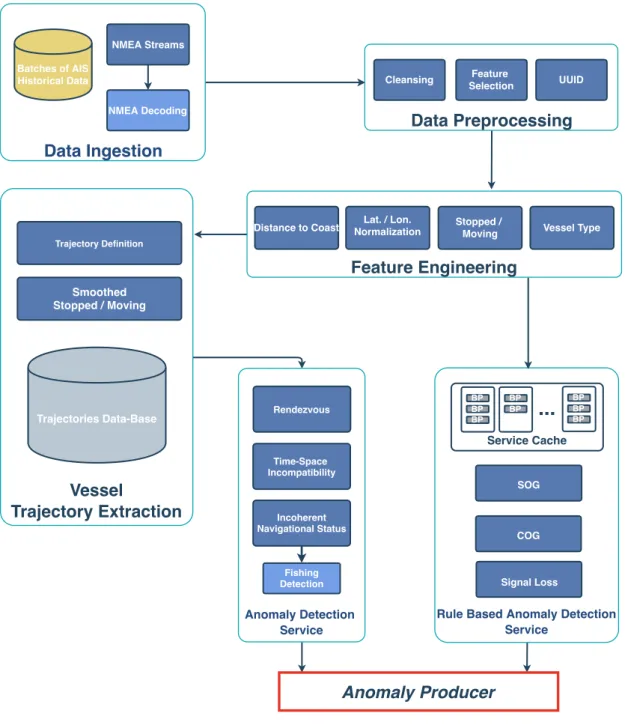
Lastly, a general overview of the proposed Modular Anomaly Detection Frame-work, which will be referred to as MAD-F from now on, is presented. This is done
in light of Figure 3.1, whose modules are explained individually throughout the following Subsections 3.2.1, 3.2.2, 3.2.3, 3.2.4, 3.2.5 and 3.2.6.
3.1
Anomalies within the MAD-F
An anomaly may have numerous interpretations depending on the context in which it is found. However, it can be generally conceptualised as a subset of data that stands out in some preconceived way when contrasted to the overall dataset. Nowa-days, the anomaly detection of vessel behaviour is solely done by human maritime experts. This procedure depends on national security agencies. Within their du-ties, these agencies are responsible for assuring the coastal surveillance of their territory by assessing possible threats and identifying abnormal behaviour. The current methods employed by these institutions are neither efficient nor scalable and therefore not suitable for the challenges brought by the exponential growth of vessels at seas. This state of affairs creates an ideal situation for the use of data-driven models to assist the maritime experts.
The notion of anomaly just presented is unsatisfactory given both the com-plexity and purpose of the problem. For the goals of this project, such a technical definition is tailored specifically by the maritime agencies involved in the Marisa project and we therefore refrain from applying our own definitions, which usually stem from abstract statistical data-driven notions.
By having meetings with maritime experts a list of the anomaly requirements was agreed. For this work this list served as not only the concrete anomaly re-quirements, but also as a guide for the overall implementation of the MAD-F. The list of anomaly requirements in shown under in Table 3.1.
Table 3.1: MAD-F anomaly requirements, which were defined by maritime officers.
Anomaly Requirement Provided Description
AR1 Detect Abnormal changes of
(more than a configurable value) Direction.
AR2 Detect Abnormal changes of
(more than a configurable value) Velocity.
AR3 Detect Vessels disappearance from sensor
coverage for more than a configurable Time Period.
AR4
Detect when the observed
Vessel Navigational Status is not consistent with the reported Vessel Kinematic features.
AR5 Detect when Vessels report a
geographical and time incompatibility.
AR6 Detect when two or more Vessels are
approaching close to each other.
As mention previously, requirements for this work were distinguished from anomaly requirements and data requirements. The latter was intrinsic for this work, as the uncertainty of data types and sources when dealing with the maritime field is immense. The problem of having numerous types and sources of data is still aggravated as the maritime domain is also capable to produce enormous workflows of data. Thus, a specific data requirement for this work could be simply specified as:
The developed Framework, must be able to ingest fuse and store different sources of maritime data, while also handling enormous workflows of data in real-time.
3.2
Modular Vessel Anomaly Detection Framework
In order to develop a Framework capable of achieving the requirements defined above in Section 3.1, we propose the Modular Vessel Anomaly Detection Frame-work. The MAD-F is able to ingest data from different feeds of data in real-time while simultaneously constructing a data-base for vessels trajectories in a unsu-pervised manner. Anomalies are then detected in a offline manner from the saved trajectory data, or online (in real time) addressing the incoming streams of vessel data. The framework was developed to be modular as there are either no inputs or outputs standards for the maritime domains. Thus, by developing a configurable and not static framework, we provide the MAD-F with the necessary configuration flexibility, allowing it to be configured for different scenarios or even by different national maritime authorities; or even allowing new Framework Modules to be easily integrated in the future.Thus, by providing a configurable and not static framework, we give the config-uration flexibility for the being configured for different scenarios or even different National Maritime Authorities, or even to new Modules being added in the future. In Figure 3.1 we present the architecture of the MAD-F and the following subsections will discuss each of the framework modules: Data Ingestion, Data Pre-processing, Feature Engineering, Trajectory Extraction and both anomaly de-tection modules : Anomaly Dede-tection Service and Rule Based Anomaly Dede-tection Service.
Vessel
Trajectory Extraction
Rule Based Anomaly Detection Service
Feature Engineering
Data Preprocessing Data Ingestion
Distance to Coast NormalizationLat. / Lon. Stopped /
Moving Vessel Type NMEA Decoding Cleansing Feature Selection Trajectories Data-Base Anomaly Detection Service Incoherent Navigational Status Anomaly Producer SOG COG Rendezvous Fishing Detection NMEA Streams Batches of AIS
Historical Data UUID
Smoothed Stopped / Moving Trajectory Definition Service Cache BP BP BP BP BP BP BP BP
...
Signal Loss Time-Space IncompatibilityFigure 3.1: Proposed architecture for the MAD-F Framework
3.2.1
Data Ingestion
Data Ingestion Module, represents the data input for the developed Framework. AIS data was the most representative data type used for this work, as it showcases the actual instantaneous Vessel information. Although, the used AIS data for this work came in two really distinct formats. It either came in Historical Batches representing historical sets of data, or real NMEA AIS Streams which represent
real, real-time data. For both data formats, the framework is scalable, and able to ingest one or multiple feeds / sources of data simultaneously.
Via the Marisa project, we accessed AIS live feeds from antennas all around the Portuguese coast line. This antennas receive vessels transmissions via AIS up to 20 Nautical Miles of the shore (depending on the weather conditions), and have reception rates up to 30 Messages per minute per vessel. The real live feeds of AIS data, are received via TCP in the NMEA format.
National Marine Electronics Association (NMEA) is a standard communica-tion protocol used by Maritime Sensors such as Accelerometer, Giroscope, GPS receivers, etc. NMEA encapsulates the information from the different Vessel sen-sors, and broadcasts this information to coastline antennas and nearby Vessels via AIS protocol.
Figure 3.2: Snapshot of raw AIS data in NMEA format.
Although the use of real AIS data comes with many challenges, as it is manda-tory to decode, sort and store the received data, thus allowing the incoming data to be used as viable source of data. Secondly, as AIS-receiving stations receive the broadcast AIS information from multiple AIS-equipped vessels simultaneously, and the reception range of each AIS-receiving can vary depending on the actual weather conditions and the location of where such station is located. This origi-nates two main problems :
1. Duplication of reception: With the variation of reception ranges from the different AIS-receiving stations, this creates the problem of multiple stations receiving the same vessel broadcast. The duplication of messages is a prob-lem which occurs when handling real NMEA streams, the methods used to solve such problem are presented in Section 4.2.
2. Non-reception of broadcast: Similar to the problem presented above the non-reception of by any receiving station can also occur. To address this problem, maritime agencies use satellite AIS (S-AIS). S-AIS solves the problems re-lated to the reception range, but presents another problem with refreshment rates, has the reception of the broadcast are dependent of satellite revisit time [24].
3.2.2
Data Pre-processing
The Data Pre-processing module, is the first step of Data Wrangling in our Frame-work. The motive for this module is to select, transform, and clean the received data, from the Data Ingestion Module. As described in Section 2.1.1, AIS presents a large amount of different features, which can be used for different problems. Fea-ture Selection represents a important step for this work, as the selection of the "relevant" features directly influences the overall performance of the MAD-F, and also the expected results from the anomaly detection task. Such representative task requires pre-conceived knowledge of Vessels dynamics and behaviour, which is only gained with experience in the Maritime Domain. For this work the feature selection was done based on the literature, and also by accessing Maritime Expert Knowledge via the Marisa project.
During the Pre-processing, a data-cleaning process is conducted, discarding corrupted data. This is done based on the information that standardises the AIS features, which is further detailed in Section 4.1.
Most importantly, in this module the concept of Behavioural Point is defined. Behavioural Point which will be referred as BP from now on, for this work repre-sents our normalised representation of the previously selected features. A detailed explanation of this concept is provided in Subsection 4.3.3.
3.2.3
Feature Engineering
Feature Engineering, represents the second step of Data Wrangling in our Frame-work. During this step, the already pre-defined BP s, in the Data Pre-processing module, are enriched by extrapolating additional features.
Firstly for each BP received by this module, if the Vessel Type is not re-ceived in the AIS message, the Vessel Type is either extracted from external vessel static information sources, or it is scrapped from this internet. Secondly, each BP is enriched with by calculating the closest country and respective distance to shore. The same is done to ports, by calculating the distance to the closest port. Also, in this module with the reported kinematic features, the instantaneous move state of the vessels is inferred. Such procedures are further individually explained throughout Subsections 4.4.1, 4.4.2, 4.4.3.
3.2.4
Vessel Trajectory Extraction
Vessel Trajectory Extraction module, handles the definition, storage, updating and inserting of new incoming BP s into defined Trajectories. When considering trajectories, the BP s stop being valued as single points in time, and the aggrega-tion of BP s via the vessel identifier throughout time, start representing a vessel trajectory. This allows a more conclusive vessel behaviour analysis based on its past trajectory. Although, in order to analyse trajectories, such concept needs to be defined and represented in a optimal manner. Furthermore, when dealing with real maritime data (and specially when working with real Maritime Authorities) it is extremely important to trace-back/log the data, thus when an a anomaly is generated, knowing which BP s generated which anomalies is possible. In Sec-tion 4.5.1 our definiSec-tion of a vessel trajectory is presented.
3.2.5
Anomaly Detection Service
ADS (Anomaly Detection Service) Module, represents for our Framework the his-torical, offline anomaly detection module. ADS module works offline in effective time, on batches of historical Trajectory Data served from Trajectory Data-Base from the Vessel Trajectory Extraction module. Access to Trajectory Data, is done by querying the Trajectory data-base with a configurable set of parameters, which can be time restrictive(such as the 10 past Hours) and or from a vessel specific set of vessels.
Received trajectory data, is then used to detect: Time Space Incompati-bility, Vessels Rendezvous, and Incoherent use AIS Navigational Status. For the latter, we create a sub-method for the which serves as the validation of Engaged at Fishing Navigational Status based on vessels types and reported kine-matic features. The implemented methodology for the detection of each anomaly is represented in Subsections 4.6.1, 4.6.2, 4.6.3 and 4.6.4 respectively.
3.2.6
Rule Based - Anomaly Detection Service
RB-ADS (Rule Based - Anomaly Detection Service), opposed to the ADS module described above, corresponds to the online, in stream processing anomaly detection module. RB-ADS modules works online in near real-time, accessing the stream of already pre-processed BP s from the Feature Engineering Module. In order to the RB-ADS be able to perform Anomaly Detection in near real-time, a Queuing Systems for this module was defined. This queue which we named Service Cache is further detailed in Section 4.7. The arriving stream of BP s, is are stored in individual Vessel Queues of size N . The individual Queues are then accessed, allowing a real-time calculation of the set of Anomaly which can be defined by Rules. The anomalies validated online trough rules for this work are: Abnor-mal change of Velocity(AR1) , the AbnorAbnor-mal change of Direction(AR2), and the Vessel Signal Loss(AR3), our approach towards the detection of such anomalies is described in Section 4.7.
MAD-F Development
In this Chapter, we present the development steps towards the implementation of the Modular Anomaly Detection Framework MAD-F. Firstly, we present a list of the technologies used in this work. Then we undertake a initial data analysis from a historical AIS dataset. And finally, the implementation of each MAD-F mod-ule is individually explained, providing a detailed clarification of the undertaken approaches.
In order not to develop a fully static framework, a modular development was applied instead. This allows specific modules of the framework to be instanced multiple times with different configuration; or even the possibility of having the new modules added to the framework in the future.
For this end the choice of technologies was done by by emphasising efficiency handling large quantities of data and scalability. Implementation of this Frame-work was done with the programming language Python, using different specific packages for the different specific tasks. The used packages and their usage will be explained throughout this Chapter. Architecturally wise, the framework was implementing following an somehow layered architecture, similar to the Lambda Architecture, which was firstly introduced by the authors in [25]. As so, the cho-sen data-base for this framework was Apache Cassandra 1, which was essential
to store the aggregated BP s in a fast and effective way. The detailed usage of the data-base is explained in 4.5. The reception of BP s by the Trajectory Ex-traction module was done using a message queue system Apache Kafka 2. The
same message queuing approach as also implemented for the modules who needed to send and consume messages between them. A detailed explanation of such implementation is provided in the following Sections.
4.1
Data Analysis
In order to gain insight and find the limitations of the AIS data, our initial step towards the implementation of the framework was a the analysis of an historical AIS dataset. The analysed dataset was compiled, and made publicly available by another H2020 European Project3. This dataset was chosen, due to the complete-ness of documentation and description of the actual dataset; which to the extend of our knowledge was the only open-source AIS dataset with such characteristics. In this Section, we present a data analysis from the dataset [26]. We conducted this data analysis, by firstly providing a general description of the used dataset, and secondly by analysing the overall feature distribution of the each feature in the used dataset. The used dataset, is composed from 18,684,115 AIS messages originated by 4,555 different vessels. The Data-Set covers a period of 6 Months (from 2015-10-01 to 2016-03-31), from a area nearby Brest, France as it is presented under in Figure 4.1.
2https://kafka.apache.org/ 3http://datacron-project.eu
Figure 4.1: Area of the dataset represented in the Red, with a sample of 50,000 AIS Positions.
Every AIS message provided in the dataset, is composed by the features that derive from the AIS dynamic information. In Table 4.1, we describe the dataset features by detailing their units and their unit range.
Table 4.1: AIS dynamic messages features description.
Feature Description Unit Range
MMSI Vessel Unique Identifier. 0 to 99999
Status AIS Navigational Status. 0 to 15
Turn Rate of turn, right or left. degrees per minute 0 to 720
SOG Speed Over Ground. knots 0 to 111*
COG Course Over Ground. degrees 0o to 360o
X Longitude. degrees -180o to +180o
Y Latitude. degrees -90o to 90o
Time Received Timestamp. Unix Time
The dataset not only contains the AIS dynamic information, but also in sep-arate files the related vessel static information of each vessel which has reported
in dataset. By interpolating the MMSI reported in every AIS message, we were able to enrich each AIS dynamic message (or row of the dataset), with the static information related to the vessel which has produced the dynamic message. The vessel’s static information contain information of the vessel’s actual dimensions and type. The use of information related to the vessels characteristics is used in different types of behavioural analysis. In this work we used the vessel type as an key aggregation indicator, which we better described in Section 4.4.1.
4.2
Data Ingestion
Data Ingestion refers to the model, where the data is input into the Framework. As mentioned in Chapter 3, for this work was assumed that the incoming data would be able to come in two different typologies, either from batches of AIS data or Live NMEA streams.
Historical batches of AIS data (or datasets), are uploaded to this module via .csv files, which then are transformed into DataFrames using the Pandas4. For each imported batch of data, the features names must be pointed to the format we present in Section 4.3.3. Although for the NMEA Streams the as the decoding of such streams was needed. The choice of methods to process and decode was not has trivial. As NMEA messages are received in high frequencies, the method to such streams into comprehensible AIS like data, needed to be stable and efficient. In order to achieve this, we used the python library libais5, which is implemented in the programming language C++, allowing a really efficient decoding of the incoming NMEA messages.
In Chapter 3, we have identified two problems that occur when working with AIS real live. In order to mitigate the duplicated reception, each received messages is tagged with a unique identifier (UUID). For this present work, the created UUID will be done by considering the ID of the vessel(MMSI), and the time the received
4https://pandas.pydata.org
message was generated by the vessel. Thus, if two same UUID messages are received, we the second messages is discarded, and only the first received messages is considered.
The Framework was developed to be scalable, being able to handle different sources of AIS data, although for the purpose of this work, we limited the used data to two main sources of Data. The Data-Set presented in Section 4.1, and the NMEA feeds made available by the Portuguese Navy.
4.3
Data Pre-processing
Data Pre-processing, represents the module that handles the raw/unprocessed AIS data. This module cleans, transforms and normalises every AIS messages, coming from the Data Ingestion Module. Every AIS message is transformed into our normalised representation of and AIS message, which we defined as a Behavioural Point, defined under in Subsection 4.3.3.
4.3.1
Latitude Longitude Normalisation
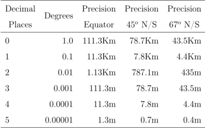
In order to normalise the reported vessels positions, either from the AIS streams or the used dataset, we defined a set number of decimal cases used. This is done as most of AIS providers only assure a GPS precision of 0.0001 minutes accuracy, but what we found was that some reported positions come with up to 8 decimal cases, which can be caused just from how the dataset files were written. So our normalisation process, we ensured that every vessel position was normalised to a precision on 4 decimal cases. As this represents a global precision error of 11m to 4m, which is shown in Table 4.2.
Table 4.2: Degree precision versus the approximate radius of measured error. Decimal Places Degrees Precision Equator Precision 45o N/S Precision 67o N/S 0 1.0 111.3Km 78.7Km 43.5Km 1 0.1 11.3Km 7.8Km 4.4Km 2 0.01 1.13Km 787.1m 435m 3 0.001 111.3m 78.7m 43.5m 4 0.0001 11.3m 7.8m 4.4m 5 0.00001 1.3m 0.7m 0.4m
4.3.2
Data Cleansing
Data Cleaning refers to the process of cleaning the data which is wrongly defined or, has wrong types. When handling with sensor generated data is common that wrong sensor reading can occur. In AIS data, this errors tend to occur as AIS features that are not transmitted at all, or that are transmitted with values that don’t correspond to the Feature value range. An example of this is having a Latitude being broadcast with values of 500o. Therefore, we discarded all AIS
messages with reported features that were not inside the feature value range. The features value range considered for the proposed framework was the one presented in Section 4.2, Table 4.1, which is similar as the one presented by the authors in [27] as the AIS default feature range.
4.3.3
Behavioural Point
Behavioural Point for this work, is our normalised feature representation of incom-ing vessel data. A BP is a multidimensional point which is identified by the vessel id who produced the reported message. Therfore a BPM M SI can be represented
as:
Where the dimensions of the multidimensional BP represents the features (Time, Longitude, Latitude, Speed Over Ground, Course Over Ground and Navigational Status) respectively. Each BP was correlated to one (one to one) identifier. The used identifier in this work was the Maritime Mobile Service Identity (MMSI). For this work the non replication of the MMSI by different vessel was assumed, this problem was discussed in Section3.2.1. Each BP , as described above is fur-ther enriched by extrapolating three additional features, making each BP to be represented as:
BPM M SI = [t, x, y, SoG, CoG, N S, V T, DtS, DtP, P N ]
Where the additional features VT, DtS, DtP, PN representing the vessel Type, Distance to Port, Distance to Shore, Port Name. These features are not reported from every AIS messages and need to be extrapolated afterwards. The methods used to extrapolated this features are presented under Section 4.4.
4.4
Feature Engineering
4.4.1
Vessel Type
Vessel Type, is a classification system, where each vessel is categorised by the type of activities it preforms. Classified by a numeric scale from 0 to 99. The first digit represents the general activity category of the vessel, and the combination of the first digit with the second represent the specific activity of the vessel. In Table 4.3 we list all the general vessel categories which are associated with the first digit of the vessel type feature, but also we present the specific vessel categories for the more frequent vessel types occurring on the dataset.
Table 4.3: Vessel Type categorisation and most frequent representation.
First Digit General Category Relevant Categories
1 Reserved
2 Wing In Ground
3 Special Category 30 - Fishing 30 - 286(6%)
4 High-Speed Craft 5 Special Category 6 Passenger 7 Cargo 70 - Cargo 70 - 1,511(33%) 79 - 273(6%) 71 - 217(5%) 8 Tanker 80 - Tanker 80 - 342(7%) 9 Other 99 - 1,192(26%)
For the used dataset described above in Section 4.1, the Static Vessel Infor-mation is available for all the vessel in the dataset. Although, when handling Real-Time NMEA streams or other Batches of Data, the Vessel Static information is not available or broadcast. This, creates a problem of not having the Vessel Type information which is used to query our Trajectory Data-Base. For this we developed a Web Scrapping application, described in the following subsection.
4.4.1.1 Vessel Type Scrapper
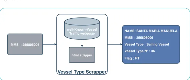
Web Scrapping is used to extract information from freely available websites. For the sole purpose of this work, we developed an application that would retrieve the Vessel Type information from a "well known vessel traffic webpage". By providing the vessel MMSI to the Vessel Type Scrapper, we retrieve the html webpage data that contains all the static vessel information available on the "well known vessel traffic webpage". From the html data we, striping the html tags, and the non
relevant specific webpage information, we access Vessel Type, as it is presented in Figure 4.2.
Vessel Type Scrapper well-Known-Vessel
Traffic webpage
MMSI : 255806006
NAME: SANTA MARIA MANUELA MMSI : 255806006
Vessel Type : Sailing Vessel Vessel Type Nº : 36
Flag : PT
html stripper
Figure 4.2: Example of the Vessel Type Scrapper retrieved information for Vessel MMSI: 255806006
4.4.2
Distance to Coast
Distance to Coast influences, the navigational behaviour for the major part of Vessel Types. In order to enrich the BP s which will feed the Anomaly Detection modules, and as the distance to shore is without a doubt a valuable aggregation feature for the maritime domain. We extrapolated the Distance to Shore for every received AIS message.
Although in order to calculate the distance to shore effectively either over historical batches of data or in real time to streams of AIS data, a efficient rep-resentation of the coastline is needed. For this we used the ocean coastline data6.
This representation has mapped Global coastline in a vector of 547,503 points, which is equivalent having a 1:10m Global coastline representation.
The calculation of the closest point was done with a Nearest Neighbour ap-proach, using the Ball Tree algorithm. The choice of this algorithm was done, due to the high volume of data we were using, and the possibility of using the Haversine Distance measures in the already implemented methods from 7.
6http://naturalearthdata.com
Haversine is the most commonly used distance metric in the vessel navigation. As both Latitude(y) and Longitude(x) features are represented in a spherical co-ordinate system, the use of the most common Euclidean distance is not applicable. Thus we used the Haversine Equation 4.1, represented under.
d = 2rsin−1 r
sin2(latp2 − latp1
2 ) + cos(latp1)cos(latp2)sin
2(lonp2 − lonp1
2 ) (4.1)
Where d takes as input (p1, p2), and it calculates the haversine the 2 point
rep-resented as p1(lat1, lon1) and p2(lat2, lon2). r represents the approximate radius
of the Earth which for this work we considered 6,367Km.
4.4.2.1 Distance to Port
Distance to Port, to the maritime scenario, and more specifically maritime inter-national trade, represents an additional feature which is of great importance. The Estimation of Time of Arrival presents itself as a necessity for container terminals, as this terminals base operational decisions on such estimation. The estimation of time of arrival, and the prediction of the arrival port based on past vessel tra-jectory information, are two tasks which use the distance to port feature for such purpose, [28, 29].
This being said, we enriched each BehaviourP oint by calculating the actual nearest port, and the distance to it. To achieve this, we used a similar approach as explained above in Subsection 4.4.2.
Although, getting a list of every port was not trivial, as there are numerous ports around the World, and such information is not centralised nor normalised. We accessed the detailed information of the World Port Indexes in 8. The World
Port Index data was in a GIS(Geographic Information System) shapefile format,
which is common format for the Maritime Domain, but not usable in our Frame-work. Therefore, we firstly normalised the data format using the Python package dbfread9, and then stored the normalised port data in our data-base. For each of
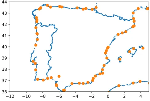
the 3,865 ports we extracted the respective Port position, Country, and Name. In Figure 4.3 we present the port position over the Iberian coast in Orange.
Figure 4.3: Iberian Ports(in orange), with the considered coastal Points(in Blue)
4.4.3
Stopped/Moving
Enriching the reported BP s by determining if at this point in time a vessel was in fact moving or stopped represents an overall information gain over the whole vessel trajectory. Such information can be used for the understanding of the normal vessels behaviour, or the detection of global points of interest. Thus, in order to gain such information, we used two different method. The first one was a point based approach, where we infer if whether a vessel is stopped or moving based on the its last report, this method is described under in this Subsection.
The second approach involves the use of a vessels past trajectory information, we present this approach further in this Chapter in Section 4.5.2.
Rule Based Approach: This approach is vastly used in the literature, as it is the simplest way to characterise the stopping of a vessel, based solely on the vessels reported speed or as reported by the AIS the Speed Over Ground (SOG). Thus, a BP which has a reported speed under a certain defined threshold ∆ is considered as stopped and the opposite are considered moving. As it is shown in equation 4.2, where BPn represents actual Behavioural Point we want extrapolate
the stopped or moving feature.
kinematicstatus(pn) = BPn.SOG > ∆; M oving BPn.SOG ≤ ∆; Stopped (4.2)
The most commonly used ∆ value found in literature was 0.5 knots. This ap-proach despite fitting most of the vessels behaviours, for the some types of fishing vessels it does not fit such behaviours. This occurs as some fishing activities, re-quire the vessel to be drastically slow down for short periods of time. In Figure 4.4, we present a fishing vessel trajectory, where the points represented in blue were to be considered as Stopped if a ∆ = 0.5 was to be considered.
Figure 4.4: Fishing vessel (MMSI: 228858000) trajectory. Where the Blue points represent the Stopped points on the overall trajectory.
4.5
Trajectory Extraction
In this Section we present our interpretation and the definition of what was for this work considered as a vessel trajectory.
4.5.1
Trajectory Definition
Representing a trajectory in a optimal way, can become a difficulty task in the maritime domain. Currently there are a vast number of solutions described in the literature. They, represent a trajectory differently, depending on the type of problem.
Our approach to represent a maritime trajectory, was to consider a trajectory as a whole. This is, as vessels are obliged to broadcast their AIS information in a semi-continuous rates. By normalising each broadcast into the defined Behavioural Point(BP ). We can aggregate each BP based on the BP sM M SI vessel identifier
which is the vessel MMSI. Thus the aggregation of BP sM M SI represents for us a
trajectory, which is represented as:
T RM M SI = BPM M SI1, BPM M SI2, BPM M SI3, BPM M SI4, · · · , BPM M SIn
Every trajectory is then sorted, and kept sorted based on the timestamp of each BPM M SI. The representation of the BP s over a time allows us to consider a each
trajectory (T RM M SI) as a multivariate time-series. Each trajectory, can be then
defined as a group of N time-series. Where N represents the number of features considered for the BP s definition.
Nevertheless, what was considered as most relevant, for our definition of a trajectory was the effectiveness, and scalability of such representation. This is, the effective adding of new BP s to a trajectory, and the accessing of historical trajectories in effective time. We achieved this by implementing the data-base in Apache Cassandra. From such we defined a set of pre-defined queries to which allowed the effective access to a whole or partial trajectory, in near real time.
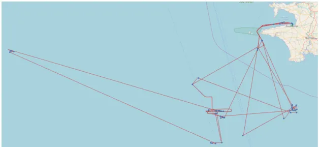
In Figure 4.5 we represent an example of the partial vessel trajectory which was plotted over a map.
Figure 4.5: Trajectory snapshot(2017-11-05 10:22 to 2017-11-05 22:42) from Vessel MMSI: 255806006
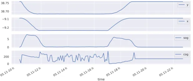
The same trajectory plotted Figure 4.5, can be also represented as a multivari-ate time-series, as it is represented in Figure 4.6. By just considering the four most relevant kinematic features of a BP , the positional features (where x represents the Longitude, and y represents the Latitude) and the speed and course features.
Figure 4.6: Trajectory represented in Figure 4.5, presented as a multivariate time-series.
4.5.2
Smoothed Stopped / Moving
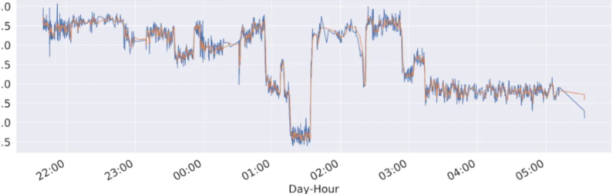
In order to resolve the problem presented in Section 4.4.3, where the rule based stopped/moving approach had problems when dealing with some type of fishing activity trajectories. And also as a trajectory could be overseen as a multivari-ate time-series. We used a commonly used time-series analysis technique, Rolling Mean. By smoothing the vessels SoG time-series, based on the previous config-urable W BP s, where W represent the window size considered. We smooth the random or abrupt variations in the observed speed features, which will in the end better describe the kinematic movement behaviour presented by these fishing vessels. The configurable W , allows the end-used of this framework, to configure the smoothness of the over the reported speed feature. This ultimately leads to a better representation of the vessel kinematics, which will be used for the anomaly detection methods presented in Subsection 4.6.1, 4.6.2 and 4.6.4.
Figure 4.7: Snapshot of Trajectory represented in Figure 4.4 SOG feature presented as a time-series.
4.6
Anomaly Detection Service
4.6.1
Time-Space Incompatibility
Time Space incompatible corresponds to an anomalous or incoherent situation where the reported actual vessels position is not compatible if compared with pre-vious reported positions, and vessels kinematics. The detection of this situation,
is also represented as an Anomaly Requirement(AR4), Section 3.1.
In order to detect this incoherence’s, we developed a method that takes as input an historical vessels trajectory T RM M SI, and for each Behavioural Point
BPM M SIT −1 we estimate the vessels position at instance BPM M SIT. The
estima-tion is done by assuming that a vessels movement can be represented in a Linear Motion. As vessels tend to move in the most economical way, the Vessels travelled distance, was calculated, using the formula:
Distance = V elocity · ∆T ime (4.3)
Where ∆T ime represents the actual time shift from point (T − 1) to (T ). The V elocity represents the BPSOG feature, which is reported in knots. The V elocity
is firstly converted to m/s. By calculating the Equation 4.3 for each BPT based on the reported Position of the previous BPT −1, and assuming a vessel tend to move
in a somewhat linear motion, we can predict that vessel should be in a distance radius of D for the next BPT, as it is shown in Figure 4.8.
(T-2) X (T-3) Y (T) D (T-1)
Figure 4.8: Linear estimation based on the previous reported BP .
By defining a configurable Distance Factor Threshold df t, representing a factor that would be multiplied by D, is possible to deduct that, if the a vessel at Time BPT is at a distance superior than (D.df t), it is considered at a incoherent position. Therefore it is reported as anomalous.
The emphasis of this Section was on the detection of Time-Space Incompatibly, which is depend on the level of error acceptance is achieved using the methods above. Although by assuming that vessels have a huge inertia, making them unable to perform quick changes of speed and direction, the authors in [30] present a Linear Estimation Algorithm. As the reported CoG represents the direction of movement, it is possible to based on Equation 4.3, to estimating the position of the Vessel, opposed to the distance from previous position. This is done by firstly calculating the Latitude and Longitude shift based on the BPT −1, using Equation 4.4.
∆X = Distance · sin(COG · π/180) ∆Y = Distance · cos(COG · π/180)
(4.4)
Where ∆X and ∆Y represent the Longitude and Latitude features shift respec-tively. Distance represents the distance which is calculated using the Equation 4.3. Finally, the estimated coordinates of the vessel are:
X0 = X + ∆X Y0 = Y + ∆Y
(4.5)
4.6.2
Navigational Status Validation
AIS Navigational Status describes the vessel current activity based on a set static set of defined status, as shown in Table 4.4.
![Figure 2.1: Three types of time series clustering defined in, [16]](https://thumb-eu.123doks.com/thumbv2/123dok_br/19177604.943894/29.893.234.714.122.524/figure-types-time-series-clustering-defined.webp)
![Figure 2.2: Difference between DTW distance and Euclidean distance (green lines represent mapping between points of time series T and S), [21]](https://thumb-eu.123doks.com/thumbv2/123dok_br/19177604.943894/31.893.280.657.638.939/figure-difference-distance-euclidean-distance-represent-mapping-points.webp)