Department of Economics
DO GREEN INSTITUTIONS MATTER? AN EMPIRICAL
ANALYSIS OF ENVIRONMENTAL PERFORMANCE IN LATIN
AMERICAN AND CARIBBEAN COUNTRIES
Etheling Alicia Alexandre Barajas
A Dissertation presented in partial fulfilment of the Requirements for the Degree of Master in Economics
Supervisor:
Prof. Catarina Roseta Palma, Associate Professor, Department of Economics. ISCTE Business School
Co-supervisor:
Sandro Mendonça, Assistant Professor, Department of Economics. ISCTE Business School
To the memory of my Father His legacy and love are always present in all my achievements
i Almighty God, the source of my strength, the Supreme Being that guides my path.
To my father, although he is no longer alive, who taught me this passion and love for numbers, and for his Portuguese heritage that brought me to this land.
To my mother, siblings, relatives and friends who are abroad, their love and support allow me to continue on this hard road.
To my sister Betsaida who I love so much, for her guidance, tenacity and support that never permit me to give up, pushing me to achieve my goals, for her advice and words that always relieve me.
To Professor Catarina Roseta Palma, for believing in me, for her help in the whole time of my Master, her lessons, and guidance, especially her support to finish the present work, Thank you so much.
To Professor Sandro Mendonça, for his ideas, enthusiasm, words, time and attention in the elaboration of this work. Muito Obrigada.
To professors, friends and colleagues that have contributed to finish my thesis, in especial to Pedro Leal and Analeda Regalado who have helped me unconditionally in this last phase to achieve this goal.
To Diego Alvarez Peiru who since I started my Master has been giving me his support, good energies and enthusiasm to always see further than the obstacles.
ii The late twentieth century presented a turning point for environmental protection. Having gained a better understanding of nature, scientists were (and still are) looking to comprehend the behavior of ecosystems, developing theories to explain the anthropogenic factors that produce negative impacts on the environment and searching for mitigating measures.
The present research explores the effects of demographic, economic and regulatory factors on environmental performance for Latin American and Caribbean (LAC) countries since 1990, putting emphasis on what that I call “green institutions” and their measurement. The notion of “green institutions” encompasses environmental bodies, agreements, norms and regulations that each country has or shares with others. These policy factors are taken to exert pressure on a wide range of aspects pertaining to environmental performance such as pollutant emissions and forest loss.
Panel data models are used for the analysis and deployed in two stages, first for all 33 LAC countries and afterwards for the major 20 countries in terms of population. The results in both stages reveal that green institutional factors do contribute to decrease deforestation, although surprisingly they also appear to increase some pollutant emissions. Such contradictory results highlight the need to develop more research in this area, using more advanced econometric techniques as well as including additional elements.
Keywords: Green Institutions, Latin America, Environmental Impacts, Ecological
Economics, Green Growth.
iii O final do século XX representou um ponto de viragem em matéria de proteção ambiental. Depois de adquirir uma melhor compreensão da natureza, os cientistas estavam (e ainda estão) à procura de um melhor entendimento do comportamento dos ecossistemas, desenvolvendo teorias para explicar os fatores antropogénicos que produzem impactos negativos no ambiente e procurando medidas de mitigação.
A presente pesquisa explora os efeitos de fatores demográficos, económicos e institucionais no desempenho ambiental dos países da América Latina e do Caribe desde 1990, enfatizando uma nova conceção de fatores institucionais, que eu chamo de “instituições verdes”, e respetiva medição. Nas instituições verdes estão incluídos órgãos ambientais, normas e regulamentos que cada país tem ou compartilha com outros, e que no seu conjunto exercem pressão sobre uma ampla gama de aspectos ambientais como emissões e desflorestação.
Modelos de dados em painel são utilizados na análise, que se dividiu em duas etapas. Os resultados obtidos em ambas as partes do trabalho revelaram que as instituições verdes contribuíram para diminuir a desflorestação, embora pareçam ter contribuído para aumentar as emissões de alguns poluentes. Estes resultados contraditórios sublinham a necessidade de desenvolver mais investigação nesta área, que usando técnicas econométricas mais avançadas, como incluindo elementos adicionais.
Palavras-chave: Instituições verdes, América Latina, Impactos Ambientais, Economia
Ecológica, Crescimento Verde. Sistema de classificação JEL: Q56, O130
iv El final del siglo XX presentó un punto de inflexión en la protección del medio ambiente. Después de haber adquirido una mejor comprensión de la naturaleza, los científicos estaban (y aún siguen) en busca de comprender el comportamiento de los ecosistemas, el desarrollo de teorías para explicar los factores antropogénicos que producen impactos negativos sobre el medio ambiente y la búsqueda de medidas de mitigación.
La presente investigación explora los efectos de los factores demográficos, económicos e institucionales sobre el rendimiento medioambiental de los países de América Latina y el Caribe desde 1990, poniendo énfasis en una nueva concepción de los factores institucionales que llamo “instituciones verdes” y sus respectivas medidas, refiriéndose con este término a los órganos ambientales, normas y reglamentos que cada país tiene o comparte con otros los cuales ejercen presión sobre una amplia gama de temas ambientales como emisiones y deforestación. Modelos de datos de panel son utilizados para el presente análisis y divididos en dos etapas. Los resultados obtenidos en las dos partes revelaron que los factores de las instituciones verdes han contribuido a disminuir la deforestación pero aumentando las emisiones contaminantes; con lo que se nota la necesidad de desarrollar más investigaciones en esta área utilizando técnicas econométricas avanzadas, así como también incluyendo otros elementos que estaban fuera de alcance.
Palabras-claves: Instituciones verdes, América Latina, Impactos Ambientales, Economía
Ecológica, Crecimiento Verde.
v
INTRODUCTION... 1
CHAPTER 1. LITERATURE REVIEW ... 3
1.1 IPAT IDENTITY. ... 3
1.2 ENVIRONMENTAL IMPACTS. ... 4
1.3 POPULATION. ... 5
1.4.AFFLUENCE. ... 5
1.5.ENVIRONMENTAL KUZNETS CURVE. ... 6
1.6.TECHNOLOGY AND OTHER FACTORS... 7
1.7.POLITICAL AND INSTITUTIONAL FACTORS. ... 7
CHAPTER 2. GOALS OF THE RESEARCH. ... 9
CHAPTER 3. LATIN AMERICA AND CARIBBEAN REGION. ... 10
2.1.LATIN AMERICA AND CARIBBEAN, A PROFILE ... 10
2.2.LATIN AMERICA UNDER ECOLOGICAL PRESSURE ... 11
CHAPTER 4. DATA AND METHODOLOGY. ... 14
4.1.ENVIRONMENTAL PERFORMANCE VARIABLES. ... 14
4.1.1. Carbon Dioxide (CO2) emissions. ... 14
4.1.2. Nitrous Oxide (NOX) emissions. ... 15
4.1.3. Ozone-Depleting Substances (ODS). ... 15
4.1.4. Percentage of forest area (Forest). ... 15
4.1.5. Summary Statistics. ... 16
4.2.DEMOGRAPHIC VARIABLES. ... 17
4.3.ECONOMIC VARIABLES. ... 18
4.4.GREEN INSTITUTION VARIABLES. ... 18
4.4.1. Multilateral environmental agreements (MEAS). ... 18
4.4.2. Year of creation of Environment Ministry (Yearmin). ... 19
4.4.3. Year of creation of general environmental law (Yearlaw). ... 19
4.5.SUMMARY STATISTICS OF INDEPENDENT VARIABLES. ... 20
vi 5.1.ALL-COUNTRIES MODELS. ... 25 5.1.1. CO2 model. ... 25 5.1.2. CO2forest model. ... 26 5.1.3. CO2percapita model. ... 27 5.1.4. NOX model. ... 28 5.1.5. ODS model. ... 29 5.1.6. Forest model. ... 30
5.2.TWENTY COUNTRIES MODELS. ... 32
5.2.1. CO2-20 model. ... 32
5.2.2. CO2percapita-20 model... 33
5.2.3. NOX-20 model. ... 34
5.2.4. ODS-20 model. ... 35
5.2.5. Forest-20 model. ... 36
5.3.DISCUSSION OF THE RESULTS. ... 37
CHAPTER 6. CONCLUSIONS ... 45
BIBLIOGRAPHY ... 47
ANNEX A. ISO 14001 MODELS. ... 51
ANNEX B. YEAR OF CREATION OF ENVIRONMENTAL MINISTRY ... 52
vii
Figure 1 The IPAT identity ... 3
Figure 2. Variables of the research ... 9
Figure 3. Latin America map ... 10
Figure 4. Sequence of steps followed for each model ... 22
Figure 5. Fixed effects model for CO2 all-countries ... 26
Figure 6. Fixed effects model for CO2forest all-countries ... 27
Figure 7.Fixed effects model for CO2percapita all-countries ... 28
Figure 8. Fixed effects for NOX all-countries model ... 29
Figure 9. Fixed effects for ODS all-countries model ... 30
Figure 10. Fixed effects for Forest all-countries model ... 31
Figure 11. Random effect for CO2-20 model. ... 33
Figure 12. Linear regression for CO2-20 per capita model ... 34
Figure 13. Linear regression for NOX-20 model ... 35
Figure 14. Random effects for ODS-20 model ... 36
Figure 15. Pooled OLS regression for Forest-20 model ... 37
Index of Tables.
Table 1Summary Stiatistics for the dependent variables of 33 countries saples ... 16Table 2. Summary Statistics for the dependent variable of 20 countries sample ... 17
Table 3. Summary statistics of independent variables for the first stage ... 20
Table 4. Summary statistics of the dependent variables for the second stage ... 21
Table 5. Name of models for the first stage ... 25
Table 6. Name of models for the second stage. ... 32
Table 7. Fixed effects models for all-countries pollutant ... 38
Table 8. OLS regressions for all-counties pollutant model ... 40
Table 9. Fixed effects an pooled OLS regression for Forest all-countries model ... 41
Table 10. Fixed and random effects model for 20 countries pollutant ... 42
Table 11. Pooled OLS regressions for 20 countries models ... 43
Table 12. Random effects and pooled OLS regression for Forest-20 model... 44
Table 13. Criteria to the Environmental Ministry Index ... 53
1
Introduction
Human activities have caused negative impacts on the environment, producing in some cases irreversible modifications on the Earth and biosphere and thereby affecting human quality of life. Many harmful actions precede our era by thousands of years (Turner, et al., 1991), although the scale of impacts has increased significantly since the beginning of the Industrial Revolution.
Before the past century, activities to protect the environment from human impacts were not given proper importance. Historical reports mention that the most degraded areas were typically abandoned (Marsh, [1864] 1965); however, the late twentieth century presented a turning point on environmental protection. Having gained a better understanding of nature, scientists were (and still are) looking to comprehend the behavior of ecosystems, developing theories to explain the anthropogenic factors that produce negative impacts on the environment and searching for mitigating measures. Economic activities play a predominant role in many of these explanatory theories, but they are not alone
Non-government movements and activities have also emerged, from international to the local scale, through a diffusion mechanism. Worldwide, regional and national institutions have been created, to regulate pernicious activities and substances. According to Frank, Hironaka, & Schofer (2000), national activities to protect the environment experienced a spectacular rise in the twentieth century.
In spite of this new conception and the rise of pro-environment activities, overall negative effects and impacts have not diminished. On the contrary, alterations of the global environment have increased dramatically in the modern era (York, Rosa, & Dietz, 2003b). Therefore exploring the factors behind environmental degradation, as well as measures to reduce it, continues to be a meaningful and fruitful research area focused on the continuing discovery, development and testing of theories that could contribute to a decline of the negative effects of anthropogenic activities on nature.
The present research explores the effects of demographic, economic and institutional factors on environmental performance for Latin American and Caribbean countries in the last twenty years, using longitudinal analysis and divided in two stages: in the first models were estimated using a sample of 33 countries and for the second the sample was reduced to 20 countries that are the most populated of the region, using in both cases the time period 1990-2011.
2 Particular features of this work are based on a new conception of institutional factors that I call green institutions and on their measuring, including with this term environmental bodies, norms and regulations that each country has or share with others, to exert pressure on a wide range of environmental issues and being responsible for environmental policy.
Although the results obtained are not always conclusive, it is clear that demographic, economic and green institutional factors have indeed impacted the environmental performance in the past twenty years for Latin American and Caribbean Countries
With the development of the present research, a first step for the region is given, bringing the need to develop more researches on this area that use the elements presented in this work with advanced econometrical techniques as well as can include other elements that were out of scope.
3
Chapter 1. Literature review
The present chapter explains some theories and works that are important to understand aspects of human society whose impact on the environment is relevant. An exploration of the new factors included in my research is also provided.
1.1 IPAT identity.
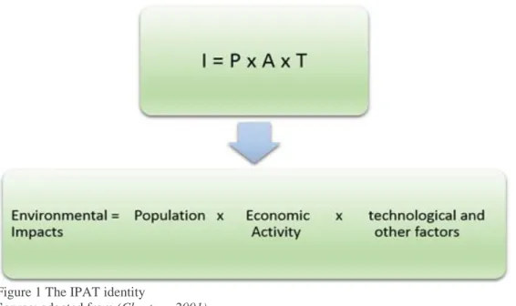
A simple expression that captures all negative impacts of society on the environment, introduced by Ehrlich & Holdren (1971), is broadly known as the IPAT identity. At first this was a relationship between population growth and a function that measured impacts per capita, depending on consumption of each individual and the technology used to produce the goods consumed.
The IPAT identity represents the fundamental features of ecological (York, Rosa, & Dietz, 2003a), expressing that the determinants of the total level of impact on the environment are function of the size of human population and per capita impacts. Figure 1 shows the identity as it is now commonly known, using affluence to refer the per capita economic activity measured as GDP per capita and technology as the amount of waste produced or resources used per unit of production (Perman, Ma, McGilvray, & Common, 2003).
Figure 1 The IPAT identity Source: adapted from (Chertow, 2001)
The identity serves as a good starting point for a statistical model, explaining the driving forces of environmental change (Dietz & Rosa, 1997). In econometric terms, the IPAT identity can
4 represent the environmental impacts as dependent variables, while population growth, affluence and technology are the independent variables. It also brings to the fore the relevance of both technological and social scientists, clarifying that not all issues are in the hands of engineers or natural scientists, as many fall into the realm of politicians and social scientists, who focus on the needs and desires of people (Chertow, 2001).
The formulation presented above allows me to express in a structured way the most important factors that my research includes, as well as highlight the new elements in my work. The following sections explain in more detail each element of the identity, how it has been used in previous work and which measures have been employed.
1.2 Environmental impacts.
Finding a unique definition or measure for environmental impact is not an easy task. In the seventies one of the first scientists who applied the IPAT concept with mathematical rigor (Chertow, 2001) was Commoner (1972), who assessed “I” as the amount of a given pollutant introduced annually into the environment; his scientific analyses were focused on measuring the amount of pollution resulting from US economic growth in the post-war era. Pollution, as a generally environmental-degradation measure, has been used, particularly after the World Resource Institute presented a restructured IPAT identity (Heaton, Repetto, & Sobin, 1991). The problem is that the environment is a complex multidimensional issue (Brunel & Levinson, 2016), and it is very difficult to use a single measure to capture all magnitudes involved. A wide number of econometric models have used diverse measures for environmental impacts as dependent variables. Works revisited for my research employ in some cases only one indicator, mainly from air quality, such as: CO2 (García, 2015), SO2 (Bernauer & Koubi, 2009; Grossman & Krueger, 1995; Leitão, 2010), or total suspended particulate (TSP), (Dasgupta, Hamilton, & Wheeler, 2006); in other environmental dimensions, the deforestation rate (Bhattarai & Hammig, 2001; Cropper & Griffiths, 1994; Culas, 2007; Enhrhardt-Martinez, 1998; Nguyen V. & Azomahu, 2007), has been broadly analysed.
Some works present results in more than one indicator (Esty & Porter, 2005; Farzin, Hossein, Bond, & Craig, 2006; Panayotou, 1993; Shafik & Bandyopadhyay, 1992); additionally, there are studies that use environmental indexes such as the Ecological Footprint (York, Rosa, & Dietz, 2003a; York, Rosa, & Dietz, STIRPAT, IPAT and ImPACT: analytic tools for unpacking the driving forces of environmental impacts, 2003b). Although all measures of
5 environmental impact have strengths and weaknesses, for my work I use Carbon Dioxide (CO2) emissions, Nitrous Oxide (NOX) emissions, Consumption of all Ozone-Depleting Substances (ODS), and percentage of forest (Forest) area.
1.3 Population.
The substantial role of population growth on environmental impacts has been demonstrated using regression analysis in several studies since the Ehrlich and Commoner studies in 1972. In some cases population growth is used directly, while in others the variable of choice is the urbanization rate (Alcott, 2012).
The term “population elasticity of impact”, referring to the responsiveness of an environmental impact to a change in population size, was tested by York, Rosa, & Dietz (2003b), who demonstrate that a change in population size is proportional and equal to one on environmental impacts.
Population size is relevant, yet a reduction in size is not a sufficient condition to reduce environmental impacts, since more resources can be used by the small number of people for economic activities, producing more pollution (Alcott, 2012); for this research population plays an important role, since in Latin America, during the past 20 years, population grew at a rate of 1.5% annually (Sheinbaum-Pardo & Ruiz, 2012). More details of the demographic characteristics of the region will be described further.
1.4. Affluence.
In the studies of Ehrlich & Holdren (1971) and Commoner (1972), affluence was defined as the amount of a particular good produced or consumed during a given year. Nowadays this term is used to represent the economic activity of a country or region, with the typical measure of such activity provided by Gross Domestic Product (GDP).
The depletion of resources (extraction), or disposal of waste (pollution) in the environment, can be seen as impacts of economic activity (Perman, Ma, McGilvray, & Common, 2003). Since the 1990’s there have been a rising number of econometric analyses of the relationship between different pollutants and economic activity (Cole & Lucchesi, 2014).
6 One of the first studies was developed by Shafik & Bandyopadhyay (1992), using 10 different indicators of environmental quality and per capita income of 149 countries. It concludes that some pollutants improve with rising income, others deteriorate then improve after a certain level of income, and others even worsen with increasing income.
1.5. Environmental Kuznets Curve.
The results of Shafik & Bandyopadhyay (1992), as well as Panayotou (1993) and Grossman & Krueger (1995), found that after countries reach a certain level of income, a turning point in per-capita emissions seems to appear, bringing the theory of an inverted U shape in the relationship between environment and income. This is known as the Environmental Kuznets Curve (EKC), after Kuznets (1955; 1963), who hypothesized an inverted U relationship between inequality in income distribution and the level of income. According to the EKC hypothesis, economic growth is therefore a means to environmental improvement.
Critics and discussions of these results emerged in 1995 and 1996 with studies of the EKC published in important journals1 such as Ecological Economics, Environment and Development Economics and Ecological Applications. These brought significant contributions to the field with the use of new explanatory variables, concluding that preliminary results had been generated in the absence of important variables.
EKC criticism can be categorized in two types: first, methodological concerns; second, criticism on the policy implications that followed (Cole & Lucchesi, 2014). Although the literature is too vast to summarize here, it should be emphasized that the EKC has been shown to apply only for a set of pollutants or impacts, not for all. Moreover, effects that cannot be reversed could appear before reaching a turning point; for instance, a secondary effect of deforestation is biodiversity loss, which is an irreversible environmental impact (Stern, Common, & Barbier, 1996).
If per capita emissions have a turning point at a certain level of income, then countries with the same level of income would show similar environmental performance. However, Esty & Porter (2005)show a wide variation in environmental performance, measured using three indicators: Urban Particulate Concentrations, Urban Sulphur Dioxide, and Energy Efficiency, confirming that income is important but does not contribute alone to ameliorate environmental outcomes.
7 The essential message from work on the EKC hypothesis is that the effect of economic development has to be taken into account for environmental improvement, but more factors are necessary for a better explanation of the anthropogenic impacts on the environment.
1.6. Technology and other factors.
Recalling the IPAT identity, population and affluence, described previously, have been more frequently covered accessible in studies than technology (T) , which has commonly been treated as the residual of an accounting identity, representing all other factors that affect the environment, additionally to population and affluence (Chertow, 2001).
Dietz & Rosa (1997), who modified the IPAT identity for a model called “Stochastic Impacts by Regression on Population, Affluence and Technology (STIRPAT)”, mentioned that T represents not only technology per se, but also culture, social organization and all facets of human life that are not explained by population and economic growth. Following this line of reasoning, my research aims to test the idea that green institutions matter for the environment, looking at a significant region of the world that has not been widely examined.
An initial effort to identify factors that determine environmental results in different countries, by Esty & Porter (2005), found that aspects of environmental regulatory regime, economic and legal context appear to significantly shape environmental performance. The preliminary evidence suggests that countries would benefit environmentally from eliminating corruption and strengthening their governance structures.
1.7. Political and institutional factors.
The effects of political and institutional factors on the environment have been tested empirically in several studies, but results have been mixed. Some research found that the quality of institutions affects environmental quality positively (Bhattarai & Hammig, 2001; Bimonte, 2002; Panayotou, 1993; Torras & Boyce, 1998), others detect no effect (York, Rosa, & Dietz, 2003a), while some show a negative impact (Harbaugh, Levinson, & Wilson, 2000). Government corruption has also been broadly studied and most results are consistent with the hypothesis that higher levels of corruption affect environmental quality negatively (Cole, Elliott, & Fredricksson, 2006; Damania, Fredriksson, & List, 2003; Fredriksson & Svensson, 2003; Fredriksson, Vollebergh, & Dijkgraaf, 2004; Leitão, 2010).
8 Dasgupta, Hamilton, & Wheeler (2006) used country corruption indices as a measure of environmental governance, with total suspended particulate (TSP) for 170 cities as a dependent variable. They found that governance helps to explain excessively high the current crisis levels of air pollution in many developing countries. Further, they provide forecasts of air pollution for 2025, with policy reforms that produce an income growth of 5%. Predictions include strong improvements in air quality for most developing-country cities, suggesting that policy reforms alone could reduce air pollution significantly.
The relationship between tropical deforestation and institutional factors was tested by Bhattarai and Hammig (2001), using political rights and civil liberties indexes to measure institutional structures. Their evidence shows that improvement in institutions leads to better conservation of forest land, reducing pressures on environmental resources in Latin America and African countries.
A fundamental idea, which arises from previous literature, is the important role that the State and its policies have in order to improve environmental outcomes. Frank, Hironaka & Schofer (2000), investigate the conditions under which nation-states have engaged in activities to protect the environment, arguing that a new dimension of state responsibility for the environment has emerged due to the emphasis of global entities on environmental protection. These new dimension of the State have created what I will refer to as green institutions. The term is meant environmental bodies, norms and regulations that each country has or share with others that exert pressure on a wide range of environmental issues and are responsible for environmental policy.
9
Chapter 2. Goals of the Research.
My research intends to analyse the effects of demographic, economic and institutional factors on environmental performance for Latin American and Caribbean countries in the last twenty years, as illustrated in Figure 2. The particular features of this work are based on the definition and measures of the performance of green institutions using indicators never used in previous work as far as I know.
Figure 2. Variables of the research
The main research goal is to develop and test an empirical model to capture the impact of demographic, economic and green institutional variables on the emissions of some pollutants and other environmental indicators, in order to ascertain whether green institutions matter. Specifically, I want to test if the year of creation of the Environmental Ministry and the year of Environmental Law was approved as well as the number of Multilateral Environmental Treaties signed by each country, have caused any effect over the environmental performance of the countries studied.
To test those effects, I choose an ecologically rich area of the World that contains particular characteristics in demographic, economic and political terms that is Lartin American and Caribbean region; before presenting the models estimated in this work, an explanation of those features will be provided in the follow chapter.
10
Chapter 3. Latin America and Caribbean Region.
The region contains particular characteristics in ecological, demographic and economic terms; richer countries in natural species such as Brazil, Colombia, Ecuador, México, Peru and Venezuela are included on the list of the countries with more biodiversity on the world (Cardozo, 2011).
In economic expressions, in 2010 an average of the rents obtained from natural resources in the worldwide was 4,72% of GDP, whereas for Latin America and Caribbean Region was 8.22% of GDP (The World Bank, 2016), it represents 1.75 times more than the world average. A general profile and principal problems that the region faces is explored in follow sections.
2.1. Latin America and Caribbean, a profile
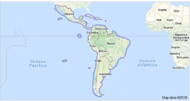
Latin America and Caribbean2 is an important region of the world that has almost 15% of the Earth’s surface area, where the majority of climates are present; the region, and specially the tropical area within it, has a rich floral and animal biodiversity (Ocampo, 1999). Geographically, Latin America covers the territory from the northern border of Mexico to the southern tip of Argentina as the map in Figure 3 shows, it is composed for thirty three states, territories and dependences.
Figure 3. Latin America map Source: (Google Map, 2016)
2 In this dissertation, the term Latin America countries is also used to refer the countries of Latin America and
11 Some of the world’s biggest rivers are in Latin America, as well as significant natural resources. Countries share common ecosystems that transcend boundaries; for instance, the Amazon jungle, Caribbean basin, Andean mountains and River Plate. Also, many migratory species of wildlife make transitory homes in several countries (Van Cott, 1999).
In demographic terms, population had an annual growth of 1.5% between 1990 and 2009; starting at 442.3 million and reaching 582.4 million inhabitants in 2009 (Sheinbaum-Pardo & Ruiz, 2012), Latin America is today a predominantly urban region, with over 80 percent of the region’s population now living in cities.
Latin America represents approximately 6.5% of the worldwide GDP (Sheinbaum-Pardo & Ruiz, 2012), with an increasing trend. However, wide differences exist among countries, so that they can be classified in three groups: high, middle and low income (Escobar, 2015). One of the most striking features of the area is the strong income inequality, with poverty still widespread; poverty and indigence rates for Latin America in 2014 were 28.2% and 11.8% for the whole population respectively (ECLAC, 2016).
2.2. Latin America under ecological pressure
Environmental problems of Latin America involve different dimensions: carbon dioxide emissions are still increasing (United Nations, 2013), biodiversity, especially in tropical areas, is still being affected by deforestation processes; marine pollution is altering natural ocean conditions (Ocampo, 1999). An achievement of the region was the decrease in consumption of ozone depletion substance during past twenty years.
Big economies in the region have specialized in natural resource exploitation implying an intensive use of land, water, energy and high rates of pollution emissions (United Nations, 2010), while the environmental costs related with this process have not been incorporated into the prices of product or services produced.
Arguably the most important problem is the insufficient economic valuation of the environmental services and stock; the idea of abundant resources led to have rates of exploitation above the natural rate of renovation (Ocampo, 1999).
12 The lack of infrastructure and effective public services has added pressure on the environment. As an example, inefficient public transport in big cities has increased the number of cars, creating traffic and air pollution, sometimes reaching critical levels such as in Mexico, Sao Paulo and Santiago de Chile. Another issue is the inadequate waste management programs, creating pollution on land, water and also air, with growing health problems and mortality rates (Ocampo, 1999).
Environmental legislation in Latin America was initially aimed at the regulation of economic activity with strong impacts (Van Cott, 1999). During the past 20 years, due to reforms and new constitutions in the majority of Latin American countries, more environmental rights and concerns have been emphasized in legislation. Today all countries of the region, without exception, have environmental legislation at a macro level, with public environmental institutions (United Nations, 2010).
In spite of the differences in many areas for each country, cooperation efforts to mitigate and preserve environmental ecosystems have been implemented. Important environmental treaties have been signed since 1940, such as the Convention of Nature Protection, organized by the Organization of American States (OAS); between 1978 and 1980; and the Amazon Cooperation Treaty, signed by Bolivia, Brazil, Colombia, Ecuador, Guyana, Peru, Suriname and Venezuela to improve the economic development and the navigation of the Amazon River, which led to the creation of an Amazon Parliament in 1989. The Central American’s National Forestry Action Program and the Agreement for the Conservation of the Biodiversity and protection of Priority Uncultivated Areas of Central America were created in the nineties. Countries in the Caribbean Region have also signed various international agreements in many varied environmental topics such as marine pollution, oil spills, protection and development of the marine environment for instance, the Caribbean Environment Program (CEP) was created by the United Nation Environment Program in 1981 and the Convention for the Protection and Development of Marine Environment was celebrated in Cartagena in 1983.
Nonetheless, advances relating to institutional change, such as institutions, treaties and laws, have been limited by the barriers presented in each country, due to an undervalued perception by politicians and citizens both of environmental amenities and of the negative impacts of the anthropogenic activities (United Nations, 2010).
On the other hand, a theoretical framework to explain institutional change in Latin America and the emerging environmental institutions of the countries therein was developed by Orihuela
13 ( 2013), two sociological theories to describe the convergences and divergences among them were used to explain different paths and the outcome of institutions: first, the sociological institutionalism that explains the homogenization of institutions and second, the historical institutionalism, referring to the political history of countries. Econometrical models to explain the relationship between those institutions and environmental impacts in Latin America are, however, not developed.
Summarizing, Latin America faces important challenges on environment issues, due to the particular characteristics of its development path: high levels of inequality and poverty, growing population a majority of which is urban; economic activities specialized in pollutant industries and natural resource depletion; delays in infrastructure development; and some advances on environmental laws and green institutions that have not had the expected outcome. All these factors make it an interesting region to study in the present research.
14
Chapter 4. Data and Methodology.
Panel data models were estimated on the present research; divided in two stages3: in the first models were built using a sample of 33 countries during the time period 1990-2011. For the second stage, the sample were reduced to 20 countries that are the most populated of the region, maintaining the same time period as in previous part.
The aim of this division was to analyse whether variables have similar impact within the most populated countries of the region. In particular, I want to analyse the importance of green institutions in this reduced sample using an index to classify the countries according to the year of creation of the Environment Ministry. The construction of this categorical variable will be explained in further sections.
Data was obtained from three main sources: the Economic Commission for Latin America and the Caribbean (ECLAC), the United Nations and the World Bank. The following sections will describe the variables, sources and transformations used for the purpose of the present work, as well as the econometrical models, procedures and tests, including results. In chapter 5 the most important analysis will be presented.
4.1. Environmental performance variables.
Environmental performance variables are the dependent variables of all models. I use three important pollutants: Total Carbon Dioxide (CO2), Nitrogen Oxide (NOX) and Ozone Depleting Substances (ODS), testing the effect of the independent variables on the emissions of each pollutant. Finally, Forest Area (Forest) is included in order to analyse deforestation, a crucial factor in the region, which has been studied by different authors (Bhattarai & Hammig, 2001; Culas, 2007; Enhrhardt-Martinez, 1998; Nguyen Van & Azomahou, 2007).
4.1.1. Carbon Dioxide (CO2) emissions.
Carbon Dioxide (CO2) is the main component of greenhouse gases; this variable indicates emissions coming from burning fossil fuels and cement production, measured in Thousands of tons of CO2. In the present work, models were regressed using both the total amount of CO2 in log form and CO2 in per capita terms for a model with per capita variables.
3 A third set of regressions involving ISO14001 was also tested with no significant results, details of this exercise
15 Several authors have used this indicator as a measure of environmental performance (Farzin, Hossein, Bond, & Craig, 2006; García, 2015; Shafik & Bandyopadhyay, 1992). Data was obtained from the Economic Commission for Latin America and the Caribbean (ECLAC, 2016).
Latin America and the Caribbean are among the group of countries that do not report their emissions of greenhouse gases, including Carbon Dioxide emissions among them. Estimates are therefore derived by the Carbon Dioxide Information Analysis Center (CDIAC), based primarily on energy statistics collected by the United Nations.
4.1.2. Nitrous Oxide (NOX) emissions.
Nitrous oxide is a trace gas that contributes to the depletion of stratospheric ozone layer while also making an important contribution to global warming. As such it has gained considerable attention in recent times (Nag, Shimaoka, Nakayama, Komiya, & Xiaoli, 2015). This variable represents emissions from agricultural biomass burning, industrial activities, and livestock management, measured in thousand metric tons of CO2 equivalent. The data was obtained from the World Bank (The World Bank, 2016), and transformed in logarithmic values
4.1.3. Ozone-Depleting Substances (ODS).
This indicator provides information of the use of substances that deplete the ozone layer controlled by the Montreal Protocol. The three major chemical compounds that contribute to the destruction of the ozone layer are: chlorofluorocarbons (CFCs), hydro chlorofluorocarbons (HCFCs) and methyl bromide (MB).
It is measured in tonnes of ozone-depleting potential (ODP), which is the unit established in the Montreal Protocol. ODP is the ratio of the impact on ozone caused by a specific substance and the impact caused by a similar mass of CFC-11 (depleting potential of CFC-11 is 1), to obtain ODP measures, each substance is multiplied by a specific factor that accounts for the ozone depletion potential. The data was obtained from the Economic Commission for Latin America and the Caribbean (ECLAC, 2016) and transformed in logarithmic form.
4.1.4. Percentage of forest area (Forest).
Forest area represents the percentage of land under natural or planted stands of trees of at least five meters in situ, whether productive or not, and excludes tree stands in agricultural production systems. With this variable I want to measure deforestation, that is, loss of forest area. Note that, unlike the previous variables, an increase in forest area is positive for the
16 environment. The data was extracted from the World Development indicators in the World Bank data (The World Bank, 2016).
4.1.5. Summary Statistics.
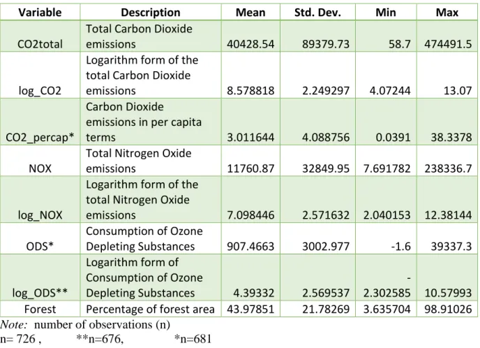
Tables presented below shows the summary statistics of the dependent variables in both stages. In Table 1 variables for the 33 countries sample as well as the names and transformations. Are presented.
Table 1Summary statistics for the dependent variables of the 33 countries sample
Variable Description Mean Std. Dev. Min Max
CO2total
Total Carbon Dioxide
emissions 40428.54 89379.73 58.7 474491.5
log_CO2
Logarithm form of the total Carbon Dioxide
emissions 8.578818 2.249297 4.07244 13.07
CO2_percap*
Carbon Dioxide
emissions in per capita
terms 3.011644 4.088756 0.0391 38.3378
NOX
Total Nitrogen Oxide
emissions 11760.87 32849.95 7.691782 238336.7
log_NOX
Logarithm form of the total Nitrogen Oxide
emissions 7.098446 2.571632 2.040153 12.38144 ODS* Consumption of Ozone Depleting Substances 907.4663 3002.977 -1.6 39337.3 log_ODS** Logarithm form of Consumption of Ozone Depleting Substances 4.39332 2.569537 -2.302585 10.57993 Forest Percentage of forest area 43.97851 21.78269 3.635704 98.91026
Note: number of observations (n)
n= 726 , **n=676, *n=681
As the table shows, observations are missing for some of the dependent variables. In such cases the econometric software employed (STATA), automatically drops the country with missing observations.
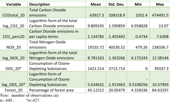
In the second stage of the research, with 20 countries, only the ODS model has missing values. The summary statistics of the dependent variables for the 20 countries are exposed in Table 2.
17
4.2. Demographic variables.
Total population and urban population are the demographic variables used for my research. Data on total population was obtained from the United Nations Population Division (United Nations, 2016) and transformed in to logarithmical form.
Table 2. Summary statistics for the dependent variable of 20 countries sample
Variable Description Mean Std. Dev. Min Max
CO2total_20
Total Carbon Dioxide
emissions 63917.3 108318.9 1052.4 474491.5
log_CO2_20
Logarithm form of the total
Carbon Dioxide emissions 9.809245 1.590859 6.958828 13.07 CO2_perc20
Carbon Dioxide emissions in
per capita terms 2.134785 1.455442 0.4734 7.6308
NOX_20
Total Nitrogen Oxide
emissions 19155.72 40530.52 479.26 238336.7
log_NOX_20
Logarithm form of the total
Nitrogen Oxide emissions 8.781163 1.363266 6.172243 12.38144 ODS_20* Consumption of Ozone Depleting Substances 1421.514 3713.714 0 39337.3 log_ODS_20* Logarithm form of Consumption of Ozone Depleting Substances 5.634631 1.913463 -0.5108256 10.57993 Forest_20 Percentage of forest area 43.12312 20.05479 4.558336 84.63297
Note: number of observations (n)
n= 440 , *n=427.
The growth rate of urban population corresponds to estimates presented by the Economic Commission for Latin America and the Caribbean Population Division (CEPAL, 2016). It is the ratio of the mean annual growth of urban population; data is only available in time period of five years, then to construct the panel data missing values were fill with the information available.
Population growth rate data is also available from Economic Commission for Latin America and the Caribbean Population Division, but it was not possible to use it on the regressions due to a high values of correlation between this and urban population growth, violating basic assumptions of Linear Regression Models (Greene, 2012).
18
4.3. Economic variables.
As noted in the literature review, the main indicator of economic activity of a country is the Gross Domestic Product (GDP), which is the value of the flow of goods and services. For my research I used the rate of growth of total annual Gross Domestic Product at 2010 constant prices.
For models where the dependent variable is CO2 per capita, it was necessary to use the rate of growth of total annual GDP in per capita terms, at constant prices. GDP data was downloaded from the Economic Commission for Latin America and the Caribbean (CEPAL, 2016). Additionally, I introduced in regressions a new economic variable which has not been considered in the literature, namely Natural Resource Rents. This variable correspond to the sum of oil, natural gas, coal (hard and soft), mineral, and forest rents, expressed as a percentage of GDP. Estimates are calculated as the difference between the world-price units of each natural resource commodity and the world average cost to produce (extract or harvest) it, multiplied by the physical quantities extracted or harvested by each country. The data source for this variable is the World Development indicators presented by the World Bank (2016). The variable is expected to contribute to impact environmental performance of the region, due to the characteristics of Latin American economies.
4.4. Green institution variables.
The main novelty of this research, however, is the inclusion of variables to measure green institutions, allowing me to verify whether these have had a detectable impact on environmental performance indicators. Given the scarcity of data on institutions, and on green institutions in particular, three new indicators were constructed: Multilateral Environmental Agreements (MEAS), year of creation of Environmental Ministry (Yearmin) and the year that general environmental law (Yearlaw) was approved in Latin American Countries. An explanation each of them is provided below.
4.4.1. Multilateral environmental agreements (MEAS).
Since most environmental problems are not confined to a single country, their mitigation requires international cooperation. Participation in multilateral environmental agreements can be seen as a policy response in each country, aimed toward a better protection of environmental goods and services in that country but with potentially wider effects. An MEA is defined as an international agreement concluded between States in written form and governed by
19 international law. For Latin America and Caribbean region, information is available from the Economic Commission for Latin America and the Caribbean on 15 different treaties.
A variable was constructed using the cumulative number of Multilateral Agreements signed by each country during the time period from 1990 to 2011. In cases where agreements were signed before the starting point of the sample (1990), the variable will take as initial value the number of treaties signed previously
4.4.2. Year of creation of Environment Ministry (Yearmin).
In the first stage of my research a dummy variable with the year of creation of the Environmental Ministry of the countries was constructed, the dummy variable takes the value of 1 from the year that Ministry was created and 0 otherwise. The information of the year of Ministry obtained from the official websites of environmental ministries4 is presented in Annex B. Year of Creation of Environmental Ministry
At the second stage, with a 20-country sample, it was observed that half of those countries had already created an Environment Ministry before 1990. For instance, the Environment Ministry of Honduras is the oldest of the region, having been created in1955. It is likely that an Environment Ministry created before 1980 would not have the same enforcement than one created in 1990. Thus I constructed a new index to categorize the countries according to the year of creation of the Environment Ministry, which I called the maturity of the Environment Ministry (MinIndx). The Annex C. Environmental Ministry Index shows the conditions used to create the index and outcomes for each country.
4.4.3. Year of creation of general environmental law (Yearlaw).
Another important aspect of green institutions is the importance accorded in national legislation to environmental issues. To assess this, I created a dummy variable with the year of creation of a general environmental law in each country, based on the document: Access to information,
participation and justice on environmental topics in Latin America, published for the Economic
Commission for Latin America and the Caribbean (2013). Considering that most environmental laws were approved during the sample period, throughout the research the dummy variable takes the value of 1 from the year a law was approved, 2 if the law had any reforms and 0 otherwise.
4 For some countries, information of the year of creation of Environmental Ministry was not available on internet;
20
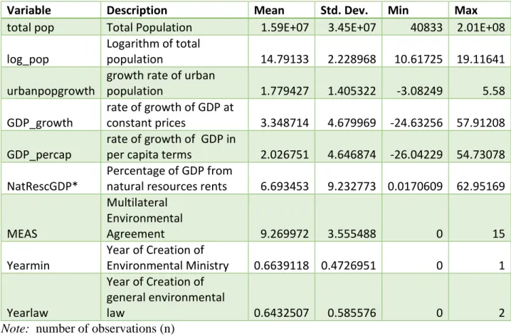
4.5. Summary statistics of independent variables.
Summary statistics for all the independent variables, a subset of which is considered in each regression for the first part of my research, are presented in Table 3.
Table 3. Summary statistics of independent variables for the first stage
Variable Description Mean Std. Dev. Min Max
total pop Total Population 1.59E+07 3.45E+07 40833 2.01E+08 log_pop
Logarithm of total
population 14.79133 2.228968 10.61725 19.11641
urbanpopgrowth
growth rate of urban
population 1.779427 1.405322 -3.08249 5.58 GDP_growth rate of growth of GDP at constant prices 3.348714 4.679969 -24.63256 57.91208 GDP_percap rate of growth of GDP in
per capita terms 2.026751 4.646874 -26.04229 54.73078 NatRescGDP*
Percentage of GDP from
natural resources rents 6.693453 9.232773 0.0170609 62.95169
MEAS Multilateral Environmental Agreement 9.269972 3.555488 0 15 Yearmin Year of Creation of Environmental Ministry 0.6639118 0.4726951 0 1 Yearlaw Year of Creation of general environmental law 0.6432507 0.585576 0 2
Note: number of observations (n)
n= 726 , *n=659.
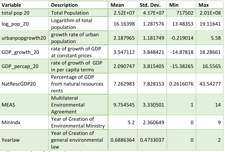
There are no missing values for the independent variables on the second stage of the research,
Table 4 presents the summary statistics of the variables employed for this subsample.
4.6. Modelling approach.
The econometric analysis of the present work is based on panel data; that is, the study handles repeated measures at different points in time of a group of units (countries, in this case), capturing variations over units and time (Cameron & Trivedi, 2009).
Panel data is interesting for econometric analysis because it allows one to learn about economic processes, taking into account heterogeneity across units as well as dynamic effects that could not be studied using cross-section or time series alone (Greene, 2012).
21 Table 4. Summary statistics of the dependent variables for the second stage
Variable Description Mean Std. Dev. Min Max
total pop 20 Total Population 2.52E+07 4.17E+07 717502 2.01E+08 log_pop_20 Logarithm of total
population 16.16398 1.287576 13.48353 19.11641 urbanpopgrowth20 growth rate of urban
population 2.187965 1.181749 -0.219014 5.58
GDP_growth_20 rate of growth of GDP
at constant prices 3.547112 3.848421 -14.87818 18.28661 GDP_percap_20 rate of growth of GDP
in per capita terms 2.090747 3.815405 -15.38265 16.5565 NatRescGDP20
Percentage of GDP from natural resources rents 7.262983 7.828153 0.2616076 43.54277 MEAS Multilateral Environmental Agreement 9.754545 3.330501 1 14
MinIndx Year of Creation of
Environmental Ministry 5.2 2.360649 0 9 Yearlaw Year of Creation of general environmental law 0.6886364 0.4733037 0 2
Note: number of observations (n)
n= 440
Longitudinal analysis employed in my research is divided in two stages. Initially models were constructed with 33 countries and a time period from 1990 to 2011; a general hypothesis to test here is if it is possible to obtain an econometric model that relates the effects of demographics, economics and green institutional features of all the countries that represent the Latin America region on the three main environmental pollutants and the effect of those features on deforestation.
The second stage was developed in order to test if the same effects appear when the sample is reduced to 20 countries using the same time period studied in the first part. Within this smaller sample there are no missing values, yet these countries represent 96% of the total population of the region, therefore they are most relevant for an understanding of policy impacts.
Modelling panel data could require complex stochastic specifications, due to the issues and violation of the classical linear models studied in econometrics. The more substantive problems are cross-observation correlation or autocorrelation (Greene, 2012), which implies that data
22 has to be well arranged and observations deserve being treated and weighted equally in order to have good quality on the panel data (Park, 2011).
Taking this in account it is important to mention that several regressions were done with Stata software for my research, and at the beginning the models presented non statistical significance, in fact, that was the reason the second stage was proposed, in order to check if significance appears in the smaller sample. Indeed, we found that the problem was solved and statistical significant models started to appear after applying logarithms to variables expressed in levels (CO2, NOX, ODS, total pop).
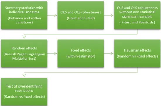
In general, for all models tests were applied in order to determine the effects of individuals and time variations over dependent variables; the Figure 4 shows the sequence followed for the data modelling, which will be explained step by step in the next paragraphs. Features of each model and discussion of the results is presented in chapter 5.
Figure 4. Sequence of steps followed for each model
In the first step, the between and within variation of dependent and independent variables were calculated. The within variation refers to the variation over time or a given individual; variations across individuals is called between variation (Cameron & Trivedi, 2009).
Linear regression model using Ordinary Least Square regression (Pooled OLS) with the option of robustness were applied for all models in the third step. The robustness corrects the correlation of the error term, because in panel data error models are very likely correlated and
23 OLS standard model assumes that errors are independent and identically distributed (Cameron & Trivedi, 2009).
Results obtained in this step allow to determine which variables are statistical significant (t-test) as well as if the model is statistical significant as a whole for a linear regression (F-(t-test). After eliminating variables that are not statistical significant in previous step, pooled OLS robustness regression was applied again in the fourth step; here I can infer if there are enough statistically significant variables to estimate a model for each dependent variable; in total 11 modes were computed. Pooled OLS regression gives the follow general equation:
𝑦𝑖𝑡 = 𝛼 + 𝑥′𝑖𝑡 𝛽 + 𝑢𝑖 + 𝜀𝑖𝑡 (1)
This regression will be the best unbiased linear estimator, as long as ui term is equal to zero, which means that individual effects are not correlated with any component of the model (Park, 2011).
In panel data, this assumption is straightforward (Cameron & Trivedi, 2009), for that reason it is necessary to test if random and fixed effects could provide better estimators.
𝑦𝑖𝑡= 𝛼+ 𝑥′𝑖𝑡 𝛽+ 𝑢𝑖+ 𝜀𝑖𝑡 (1) is not correlated with regressors (x′it β) and ui is correlated with the error component term (εit). In this case the model is written in the follow form:
𝑦𝑖𝑡 = 𝛼 + 𝑥′𝑖𝑡 𝛽 + (𝑢𝑖 + 𝜀𝑖𝑡) (2)
The Breusch-Pagan Lagrange Multiplier (LM) test examines if individual or time specific variances are zero; thus rejecting the null hypothesis is possible to conclude that there is a significant random effect in the panel data and this is better than pooled OLS model (Park, 2011).
A limited form of endogeneity also is tested in the sixth step, using the fixed effect model. In this part α from (1) has two components: one that is correlated with ui , the other that is time invariant and correlated with regressors (x′it β). The assumption that estimators are not
24 correlated with the random component error term (εit) holds. In that type of models the general equation can be written as:
𝑦𝑖𝑡 = ( 𝛼 + 𝑢𝑖) + 𝑥′𝑖𝑡 𝛽 + 𝜀𝑖𝑡 (3)
In order to test if fixed effects model for the data, within estimator is computed, rejecting the null hypothesis of the F-test allow to infer that fixed effects model is statistical significant (Cameron & Trivedi, 2009).
Outcomes of the last two previous steps could give that fixed and random effects are statistical significant for panel data model, being necessary to test which of is more relevant for the sample.
The seventh step Hausman test is applied to determine which of those effects significant. In this test the null hypothesis is that random effects is preferred over fixed effects (Park, 2011), then rejecting the null hypothesis fixed effects model is relevant for the panel data.
Finally the last step was applied, when some problems arise computing the Hausman test; especially when different estimates of the error variance produce failures on the significance (Cameron & Trivedi, 2009). In order to obtain a result between the relevance of fixed and random effects the xtoverid command in Stata is applied, using a similar assumption of the Hausman test.
25
Chapter 5. Empirical application.
The tests applied for the eleven models and their results are presented in this chapter, separating the models into two parts: the first discusses the six models regressed for all the countries of the region and the second part corresponds to five models regressed just for 20 countries; the results presented will be discussed at the end of the chapter.
5.1. All-countries models.
Six models were estimated in this part of the research. Since the software dropped those countries that have missing values in natural resources GDP, the sample was reduced to 30 countries and 659 observations. Table 5 summarizes the name used for each model as well as the dependent variable that characterises. In this part of the research, the Hausman test applied for all models revealed that fixed effect is preferred over random effects, the outputs of the test are reported in follow sections.
Table 5. Name of models for the first stage
Num. Name of Model Dependent variables.
1 CO2 Logarithm form of the total Carbon Dioxide emissions
2 CO2forest
Logarithm form of the total Carbon Dioxide emissions using the percentage of forest area as independent variable
3 CO2percapita Carbon Dioxide emissions in per capita terms
4 NOX Logarithm form of the total Nitrogen Oxide emissions 5 ODS Logarithm form of Consumption of Ozone Depleting
Substances
6 Forest Percentage of forest area
5.1.1. CO2 model.
The pooled OLS regression reported that the growth rate of GDP, multilateral environmental agreements and general environmental law (GDP_growth, MEAS, Yearlaw) are not statistical significant variables. The model presented the follow form:
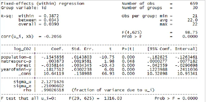
26 Tests for random and fixed effects gave that both models are statistical significant, in Hausman test, the null hypothesis was rejected which implies the presence of a limited endogeneity, as I explained in section 4.6 and fixed effects are preferred over random effects model. The results of fixed effects are presented in Figure 5.
Figure 5. Fixed effects model for CO2 all-countries Source: Stata Outputs
As we can see in the figure, natural resources GDP becomes statistically insignificant in this model whereas in pooled OLS regression the coefficient for this variable has a value of 0.088 (p=0.000). In the discussion of the results tables with the respective coefficients for fixed and pooled OLS models are explained in detail.
5.1.2. CO2forest model.
This is an extension of the previous model using the percentage of forest area as an independent variable; forest area also is used later as dependent variable. Forest and the same variables used in previous model are statistically significant in the pooled OLS regression test. Residual square errors of this model is higher in comparison with total CO2 emission (0.4045 vs 0.372). The functional form of the model presented is:
27 As in previous model, tests applied for random and fixed effects presented that both models are statistical significant being preferred the fixed effect over random when Hausman test is computed. Results of the fixed effects are displayed in Figure 6.
Figure 6. Fixed effects model for CO2forest all-countries Source: Stata Outputs
All variables become statistical significant, the sign of the estimator of forest area is the expected in line with the theory that increasing forest area can contribute to the reduction of Carbon Dioxide emissions, if all others factors remain constant.
5.1.3. CO2percapita model.
Using the data of per capita Carbon Dioxide emissions I regress a model for this variable, in pooled OLS variables GDP_growth, MEAS and Yearlaw shows again do not have a statistical significant impact that can explain per capita emissions of Latin America Countries. The model estimated can be written as it follows:
28 Regarding the outcomes of the tests applied to this panel data, the fixed effects model seems to be the proper one in comparison with random effect. Figure 7 exhibits the outcomes of fixed effect for CO2 per capita model.
Figure 7.Fixed effects model for CO2percapita all-countries Source: Stata Outputs
As we can see estimators for variables Forest and Yearmin become non statistical significant, whereas in pooled OLS both are significant, having the same sign than in fixed effects. A comparison of outcomes will be presented in section 5.3. Discussion of the results.
Until now, in all models regressed for carbon dioxide emissions of Latin American countries the same four variables resulted statistical significant: growth rate of urban population, natural resources rents, forest area and the year of creation of environmental ministry.
According to the fixed effects models’ outputs, the growth rate of population shows negative sign in the three estimations which implies that increasing the growth rate of urban population can contribute on the reduction of the emissions if all other variables remain constant.
5.1.4. NOX model.
Once more in pooled OLS regression GDP_growth, MEAS and Yearlaw are not statistical significant to explain the dependent variable. A general representation of the Nitrous Oxide emissions model can be expressed as:
29 In Figure 8 results of fixed effects are presented, the null rejection of the hypothesis for fixed and random effect models indicates that both are significant. After computing Hausman test a preference for fixed effects is revealed, indicating that α from 𝑙𝑜𝑔𝑁𝑂𝑋= 𝛼 +
𝛽1𝑢𝑟𝑏𝑎𝑛𝑝𝑜𝑝𝑔𝑟𝑜𝑤𝑡ℎ + 𝛽2𝑁𝑎𝑡𝑅𝑒𝑠𝑐𝐺𝐷𝑃 + 𝛽3𝑌𝑒𝑎𝑟𝑚𝑖𝑛 + 𝜀𝑡 (6) is also related with estimators.
Figure 8. Fixed effects for NOX all-countries model Source: Stata Outputs
Urban population and the year of environmental ministry present a positive effect on the Nitrous Oxide emissions, it can be seen as a negative impact for the environmental quality. The percentage of GDP for natural resources rents has the opposite effects.
5.1.5. ODS model.
As in previous model the same variables: GDP growth rate, MEAS and Yearlaw, are also non statistical significant. In general form this model can be written as:
𝑙𝑜𝑔𝑂𝐷𝑆= 𝛼 + 𝛽1𝑢𝑟𝑏𝑎𝑛𝑝𝑜𝑝𝑔𝑟𝑜𝑤𝑡ℎ + 𝛽2𝑁𝑎𝑡𝑅𝑒𝑠𝑐𝐺𝐷𝑃 + 𝛽3𝑌𝑒𝑎𝑟𝑚𝑖𝑛 + 𝜀𝑡 (7)
Random effects and fixed effects are statistical significant for the model, the null rejection for Hausman test indicates that fixed effects are preferred over random effects model, Figure 9 exhibits the outputs for fixed effect model.
30 Figure 9. Fixed effects for ODS all-countries model
Source: Stata Outputs
Natural resources rents shows negative sign implying that an increase in the percentage of this variable will contribute to diminish the consumption of the depletion substances if all other variables remain constant. The dummy variable year of environmental ministry presents a negative sign in fixed effects model but positive sign in pooled OLS regression.
For the pollutant emissions studied until now a similar pattern is founded: the same independent variables and the same effects model can appear to be related in the analysis of the environmental performance of all countries of Latin America. The pattern observed allow me to infer that at least one variable for each element explained in the theoretical part is significant, arguing that demographic, economic and institutional factors have an impact on the environment.
5.1.6. Forest model.
Results of pooled OLS shows that the growth rate of GDP is not statistical significant neither multilateral environmental agreements, the rest of the variables tested revealed a relationship with the percentage of forest area. The model can be described in as the equation presented below.
𝐹𝑜𝑟𝑒𝑠𝑡 = 𝛼 + 𝛽1𝑙𝑜𝑔𝑝𝑜𝑝+ 𝛽2𝑢𝑟𝑏𝑎𝑛𝑝𝑜𝑝𝑔𝑟𝑜𝑤𝑡ℎ + 𝛽3𝑁𝑎𝑡𝑅𝑒𝑠𝑐𝐺𝐷𝑃 + 𝛽4 𝑌𝑒𝑎𝑟𝑚𝑖𝑛 + 𝛽5𝑌𝑒𝑎𝑟𝑙𝑎𝑤 + 𝜀𝑡 (8)
31 Following the procedure applied for previous models, tests for fixed and random effects were computed, the outcomes indicates that both models are statistical significant, being necessary run the Hausman test to determine that fixed effects model can be better than random effects. Outputs of fixed effect regression is displayed in Figure 10.
Figure 10. Fixed effects for Forest all-countries model Source: Stata Outputs
As we can see in the outputs population growth rate and urban natural resources rents become non statistical significant for fixed effects. It is important to mention the roll that year of environmental law is playing, the variable indicates a positive effect over the percentage of forest area. Once more, the dummy variable year of ministry presents a negative sign in fixed effects model but positive sign in pooled OLS regression.
Until now all-countries models have been presented with their results; before explaining the second part of my research it is important to mention some conclusions obtained: the first is that the same independent variables have impact on the three pollutant emissions studied, representing all the elements that my research cover, second the year of creation of environmental ministry appears significant in all models computed until now, the positive sign per capita emissions of carbon dioxide indicates that the presence of ministry have contribute