Ricardo Jorge Guerreiro Antunes

(1)

Automatic delimitation of the clinical region of

interest in ultra-wide field of view images of the

retina

Dissertação para obtenção do Grau de Mestre em Engenharia Biomédica

Orientador: André Damas Mora, FCT, UNL

Júri:

Presidente: Carla Quintão, FCT, UNL Arguente(s): Pedro Vieira, FCT, UNL

(2)

s

Ack

n

owledgem

en

ts

A

Automatic delimitation of the clinical region of interest in ultra-wide field of view images of the retina Ricardo Antunes

2

0

1

(3)

gia, Universidade Nova de Lisboa.

A Faculdade de Ciências e Tecnologia e a Universidade Nova de Lisboa têm o direito, perpétuo e sem limites geográficos, de arquivar e publicar esta disserta-ção através de exemplares impressos reproduzidos em papel ou de forma digital,

(4)

(5)

Acknowledgements

To my advisor I want to thank for letting me do this thesis, for giving me the independence to find my own solutions to the problems which were pre-sented and mostly for the amazing patience and personality and for being there whenever I need to.

To Manuel Coelho I want to thank for the amazing electric kettle which

proportionate the amazing tea to free both our minds in the beginning and for company provided on those afternoons.

To Nuno Figueiredo for all those shared nights in the UNL-FCT and great mood which end up revealing to be so important to make sure this thesis were finalized in time.

To all my friends who were always there to make sure I don’t got out of line to many times and to make sure I got out when needed, for all the advices and always being an example to follow I have to truly thank with all my heart.

(6)

(7)

Retinal ultra-wide field of view images (fundus images) provides the visu-alization of a large part of the retina though, artifacts may appear in those images. Eyelashes and eyelids often cover the clinical region of interest and worse, eye-lashes can be mistaken with arteries and/or veins when those images are put through automatic diagnosis or segmentation software creating, in those cases,

the appearance of false positives results.

Correcting this problem, the first step in the development of qualified auto-matic diseases diagnosis programs can be done and in that way the development of an objective tool to assess diseases eradicating the human error from those processes can also be achieved.

In this work the development of a tool that automatically delimitates the clinical region of interest is proposed by retrieving features from the images that will be analyzed by an automatic classifier. This automatic classifier will evaluate the information and will decide which part of the image is of interest and which part contains artifacts.

The results were validated by implementing a software in C# language and validated through a statistical analysis. From those results it was confirmed that the methodology presented is capable of detecting artifacts and selecting the

clin-ical region of interest in fundus images of the retina.

Keywords: clinical ROI, fundus images, retina, artifacts, eyelashes, eyelids,

(8)

(9)

Imagens de campo alargado da retina proporcionam a visualização de grande parte da mesma, no entanto grande parte das imagens apresentam arte-factos. É frequente o aparecimento tanto de pestanas, como de pálpebras nas ima-gens cobrindo desse modo a zona de interesse clínico e, pior, podendo as pesta-nas ser confundidas com artérias ou veias, quando estas imagens são sujeitas a

programas de diagnóstico ou segmentação automática.

Corrigindo este problema, estará dado o primeiro passo no desenvolvi-mento qualificado de programas automáticos de diagnóstico de doenças e dessa forma também de uma ferramenta objetiva livre de erros subjetivos associados à presença humana.

Neste trabalho é proposto o desenvolvimento de uma ferramenta que deli-mite automaticamente a região de interesse clínica retirando, das imagens, carac-terísticas. Características essas que serão apresentadas a um classificador auto-mático que avaliará a informação e decidirá se esta pertence ou não à zona de interesse da imagem.

Os resultados foram validados através da implementação de um software

em linguagem C# e foram confirmados segundo uma análise estatística. Desses resultados surgirá a confirmação de que a metodologia apresentada neste

traba-lho foi a correta para a deteção de artefactos e para a delimitação automática da região de interesse clínica em imagens do fundo da retina.

(10)

(11)

-List of Tables

TABLE 3.1-RESULTS OF RED CHANNEL LOWEST PIXEL INTENSITY BEFORE THE BRIGHTNESS AND CONTRAST

CORRECTION. ... -25

-TABLE 3.2-RESULTS OF RED CHANNEL LOWEST PIXEL INTENSITY AFTER THE BRIGHTNESS AND CONTRAST CORRECTION. ... -26

-TABLE 3.3-RESULTS OF RED CHANNEL PIXEL INTENSITY BEFORE THE BRIGHTNESS AND CONTRAST CORRECTION. ...-27 -TABLE 3.4-RESULTS OF RED CHANNEL PIXEL INTENSITY AFTER THE BRIGHTNESS AND CONTRAST CORRECTION. . -28

-TABLE 3.5-RESULTS OF GREEN CHANNEL PIXEL INTENSITY BEFORE THE BRIGHTNESS AND CONTRAST CORRECTION ..-28 -TABLE 3.6-RESULTS OF GREEN CHANNEL PIXEL INTENSITY AFTER THE BRIGHTNESS AND CONTRAST CORRECTION. ...-29 -TABLE 3.7-RESULTS OF MAGNITUDE FFT BEFORE THE BRIGHTNESS AND CONTRAST CORRECTION. ... -30

-TABLE 3.8-RESULTS OF FFT MAGNITUDE AFTER THE BRIGHTNESS AND CONTRAST CORRECTION. ... -31

-TABLE 5.1-MEAN SENSITIVITY AND SPECIFICITY. ... -50

-TABLE 5.2-MEAN PPV AND NPV. ... -51

-TABLE 5.3-MEAN ACCURACY AND PRECISION. ... -52

-TABLE 5.4-MEAN FP AND FN. ... -53

-TABLE 5.5-COST MATRIX FOR FP AND FN. ... -53

-TABLE 7.1-FIRST DATA COMPARING RESULTS ACCORDING TO THE NUMBER OF BLOCKS CROPPED FROM THE IMAGE FOR THE GREEN CHANNEL AND MAGNITUDE FFT CHARACTERISTICS. ... -67

-TABLE 7.2-FIRST DATA COMPARING RESULTS ACCORDING TO THE NUMBER OF BLOCKS CROPPED FROM THE IMAGE FOR THE RED CHANNEL CHARACTERISTICS. ... -71

-TABLE 7.3-FALSE POSITIVE AND FALSE NEGATIVE ERROR PER IMAGE BEFORE SETTING THE BETTER NUMBER OF BLOCKS. ... -74

(14)

-TABLE 7.7-DATA OF THE GREEN CHANNEL AND MAGNITUDE FFT CHARACTERISTICS AFTER CONTRAST AND

BRIGHTNESS CORRECTION. ... -81 -TABLE 7.8-DATA OF THE RED CHANNEL CHARACTERISTICS AFTER CONTRAST AND BRIGHTNESS CORRECTION. .. -83 -TABLE 7.9-FALSE POSITIVE AND NEGATIVE ERROR PER IMAGE AFTER CONTRAST AND BRIGHTNESS CORRECTION. ....

-84

-TABLE 7.10-FINAL DATA OF FP,FN,TP AND TN OF ALL IMAGES. ... -85 -TABLE 7.11-FULL DATA OF SPECIFICITY, SENSITIVITY, ACCURACY, PRECISION,PPV AND NNV VALUES OF ALL

(15)

-FIGURE 1.1-COMPARISON BETWEEN STANDARD AND ULTRA-WIDE FIELD IMAGING OF THE RETINA.(A)ETDRS7

STANDARD FIELD IMAGE (45º);(B)ULTRA-WIDE FIELD OF VIEW IMAGE. ... -1

-FIGURE 1.2–HORIZONTAL SECTION OF THE EYE.(DAVSON,1980) ... -2

-FIGURE 1.3-MAIN COMPONENTS OF THE EYE... -3

-FIGURE 1.4-IMAGE OF THE EYE AND ITS COMPONENTS WITH SPECIAL EMPHASIS FOR THE RETINA. ... -4

-FIGURE 1.5-FUNDUS IMAGE OF THE RETINA WITH THE OPTIC DISC AND MACULA IN EVIDENCE. ... -4

-FIGURE 1.6-OPTOSOPTOMAPMACHINE ... -5

-FIGURE 1.7-ULTRA-WIDE FIELD IMAGING RANGE GIVEN BY OPTOMAP TECHNOLOGY. ... -6

-FIGURE 1.8-COMPARISON BETWEEN THE TWO MONOCHROMATIC SLO, RED AND GREEN SCANS.(A)GREEN CHANNEL IMAGE;(B)RED CHANNEL IMAGE. ... -6

-FIGURE 1.9-ULTRA-WIDE FIELD IMAGING OF A NORMAL RETINA. ... -8

-FIGURE 1.10-CONSEQUENCES OF DIABETIC RETINOPATHY. ... -9

-FIGURE 1.11-COMPARISON BETWEEN THE TWO TYPES OF DIABETIC RETINOPATHY.(A)NON-PROLIFERATIVE DIABETIC RETINOPATHY;(B)PROLIFERATIVE DIABETIC RETINOPATHY. ... -10

-FIGURE 1.12-OPTOMAP IMAGE OF AN EYE WITH DIABETIC RETINOPATHY... -11

-FIGURE 1.13-OPTOMAP IMAGE OF AN EYE WITH BRVO. ... -12

-FIGURE 1.14-OPTOMAP IMAGE OF AN EYE WITH UVEITIS. ... -13

-FIGURE 1.15-EXAMPLE OF A FUNDUS IMAGE WITH EYELASHES AND EYELIDS COVERING MOST OF THE ROI(REGION OF INTEREST) OF THE RETINA. ... -14

-FIGURE 1.16-EXAMPLE OF AN EXPECTED RESULT OF THE SOFTWARE PROPOSED IN THIS THESIS. ... -15

-FIGURE 3.1-METHODOLOGY FOR AUTOMATIC DELIMITATION OF THE CLINICAL ROI IN ULTRA-WIDE FIELD OF VIEW IMAGES OF THE RETINA. ... -22

-FIGURE 3.2-COMPLETE PROCESS (STEP BY STEP) FOR AUTOMATIC DELIMITATION OF THE CLINICAL ROI IN ULTRA -WIDE FIELD OF VIEW IMAGES OF THE RETINA. ... -22

-FIGURE 3.3-IMAGE PRE-PROCESSING PHASE WITH ALL ITS METHODS AND STAGES DETAILED. ... -24

-FIGURE 3.4-ORIGINAL IMAGE BEFORE THE BRIGHTNESS AND CONTRAST CORRECTION. ... -25

-FIGURE 3.5-ORIGINAL IMAGE AFTER BRIGHTNESS AND CONTRAST CORRECTION.(A)ORIGINAL IMAGE AFTER THE CONTRAST BEING DECREASED;(B)ORIGINAL IMAGE AFTER THE CONTRAST BEING DECREASED AND BRIGHTNESS BEING INCREASED. ... -26

-FIGURE 3.6-ORIGINAL IMAGE AFTER BRIGHTNESS AND CONTRAST CORRECTION.(A)ORIGINAL IMAGE AFTER THE CONTRAST BEING DECREASED;(B)ORIGINAL IMAGE AFTER THE CONTRAST AND BRIGHTNESS BEING DECREASED. ... -27

-FIGURE 3.7-ORIGINAL IMAGE AFTER BRIGHTNESS AND CONTRAST CORRECTION.(A)ORIGINAL IMAGE AFTER THE CONTRAST BEING SLIGHTLY DECREASED;(B)ORIGINAL IMAGE AFTER THE CONTRAST AND BRIGHTNESS BEING DECREASED. ... -29

(16)

-WORKS PURPOSE. ... -31

-FIGURE 3.10-REVERSING THE ORIENTATION OF THE IMAGE.(A)ORIGINAL IMAGE;(B)ORIGINAL IMAGE CORRECTLY INVERTED. ... -32

-FIGURE 3.11-REGION CONTAINING THE OPTIC DISC;IMAGE ABOVE IN VALUES;IMAGE BELOW IN COLORS. ... -33

-FIGURE 3.12-IMAGE DIVIDED INTO 400(20X20) SMALL IMAGES. ... -34

-FIGURE 3.13-RED CHANNEL AVERAGE PIXEL INTENSITY VALUES PER BLOCK. ... -34

-FIGURE 3.14-STRUCTURE OF THE IMAGE PROCESSING PHASE AND ITS METHODS. ... -35

-FIGURE 3.15-STRUCTURE OF THE IMAGE POST-PROCESSING PHASE AND ITS METHODS. ... -36

-FIGURE 3.16–BINARIZED IMAGE AFTER OTSUTHRESHOLDING. ... -37

-FIGURE 3.17–RESULTING ROI OF AGGREGATION ALGORITHM... -38

-FIGURE 3.18–FIRST CROSSING RESULTING ROI. ... -38

-FIGURE 3.19-FINAL CROSSING RESULTING ROI. ... -39

-FIGURE 4.1-GRAPHICAL USER INTERFACE (GUI) OF THE AUTOMATIC DELIMITATION OF THE CLINICAL ROI SOFTWARE. ... -41

-FIGURE 4.2-RESULTING IMAGE WITH THE GRID SELECTED. ... -42

-FIGURE 4.3-DETAILED GUI. ... -43

-FIGURE 4.4-IMAGE CROPPED INTO 144(12X12) BLOCKS WITH VALUE AND COLOR VISUALIZATION OF THE RED CHANNEL LOWEST PIXEL INTENSITY VALUE AND COLOR BY BLOCK... -44

-FIGURE 4.5–FEATURES LIST OF THE SELECTED IMAGE BLOCK. ... -45

-FIGURE 5.1-GRAPHICS OF SENSITIVITY AND SPECIFICITY PER IMAGE. ... -50

-FIGURE 5.2-GRAPHICS OF NPV AND PPV PER IMAGE. ... -51

-FIGURE 5.3-GRAPHICS OF ACCURACY AND PRECISION PER IMAGE. ... -52

-FIGURE 5.4-GRAPHICS OF FP AND FN PER IMAGE. ... -53

(17)

Acronyms

ANN - Artificial Neural Network

BRVO - Branch Retinal Vein Occlusion

DR – Diabetic Retinopathy

ETDRS – Early Treatment of Diabetic Retinopathy Study

FFT - Fast Fourier Transform

FN - False Negative

FP - False Positive

GUI - Graphical User Interface

HRVO - Hemi-central Retinal Vein Occlusion

NPV - Negative Predictive Value

PPV - Positive Predictive Value

ROI - Region Of Interest

SLO - Scanning Laser Ophthalmoscopy

TN - True Negative

(18)

(19)

Chapter 1. Introduction

Ultra-wide field imaging, more specifically OPTOMAP, due to its effectiveness and large view of imaging , is becoming more clinically accepted and used over the standard ETDRS (Early Treatment of Diabetic Retinopathy Study) method of 7 standard fields of imaging, as it allows for the capture of one single image cov-ering about 200º of the retina’s surface. With this technology it is possible to vis-ualize the central and periphery of the retina in the same image (Figure 1.1).

Figure 1.1 - Comparison between standard and ultra-wide field imaging of the retina. (a) ETDRS 7 standard field image (45º); (b) Ultra-wide field of view image.

However certain artifacts often appear in those pictures. Eyelashes by being visible and eyelids by covering part of the retina make an automatic diagnosis very difficult.

(20)

This thesis main goal is to delineate the area containing these artifacts, by iden-tifying and classifying the main features in ultra-wide field of view images, thus allowing automatic diagnostic to perform without errors.

The following sections will introduce the theoretical concepts to fully under-stand this thesis work.

1.1 Human Eye

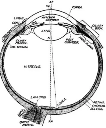
The human eye (Figure 1.3) can be considered as being composed by three layers involving the liquid center, vitreous body and aqueous humor, responsible for the refraction (Figure 1.2). The outer layer, responsible for the protection, is consisted by the sclera and the transparent cornea. The middle layer with mainly

vascular functions is composed by the choroid, ciliarybody and iris. The retina, re-sponsible for the vision, is located in the inner layer (Davson, 1980).

Figure 1.2 – Horizontal section of the eye. (Davson, 1980)

The aqueous humor main function is to provide the crystalline lens and the

(21)

is to provide the necessary refraction and to fill the eye cavity. The sclera, com-posed by dense collagen fibers, holds together the contents of the eye and the

cornea is responsible for most of the eye’s focusing power. The choroid, rich in

blood vessels, provides the nourishment for the retina’s photoreceptors, the cili-arybody and the iris make up the uvea, the iris open middle region is known as

pupil and its size adjusts the level of light and accommodation (Lens, Nemeth, & Ledford, 2008).

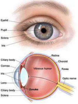
Figure 1.3 - Main components of the eye.

1.2 Retina

The retina is the part of the eye responsible for detecting light, transforming photon energy in electrical pulses that will later be interpreted by the brain. The retina has two kinds of photoreceptor cells, the rods and the cones. Rods are the most predominant (about 75 to 150 million cells) and they are very sensible to light but not to color, providing little detail. Cones are less abundant (about 6 to

(22)

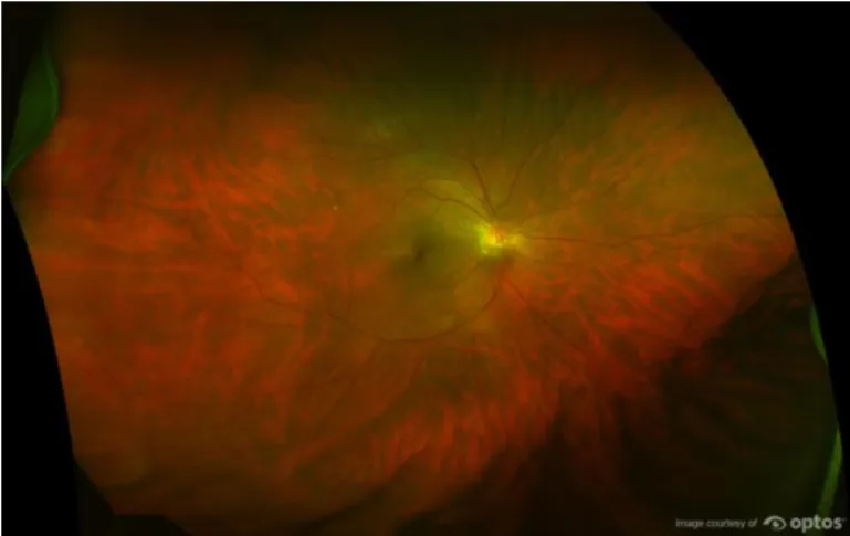
In the center of the retina there is a circular to oval white area measuring about 2x1.5 mm that is the optic disc which contains the optic nerve (here there aren’t

any photoreceptor cells, being then commonly known as “blind spot”) from where the major blood vessels of the retina are radiated. At the left of the disc it can be seen a slightly oval-shaped, blood vessel-free reddish spot, the fovea, which is at the center of the area responsible for the central vision known as the macula. A circular field of approximately 6 mm around the fovea is considered the central area of the retina while from there is considered the peripheral area of the retina, stretching to the ora serrata (anterior boundary of the retina), ap-proximately 21 mm from the center of the fovea. The total retina is a circular disc of between 30 and 40 mm in diameter (Figure 1.4).

Figure 1.4 - Image of the eye and its components with special emphasis for the retina.

Figure 1.5 - Fundus image of the retina with the optic disc and macula in evidence. MACULA

(23)

1.3 Ultra-Wide Field Scanning Laser Ophthalmoscopy (OPTOMAP)

Ultra-wide field of view imaging (fundus imaging) technology allows that ei-ther the central and peripheral (less considered) parts of the retina to be visual-ized in the same image.

This technology of ultra-wide field scanning laser ophthalmoscopy (OPTO-MAP) (Figure 1.6) when applied to the retina allows a 200⁰ (Figure 1.7) retinal fundus image to be capture in a single picture, representing approximately 82% of the retinal area, with an acquisition time of 0.25 seconds, thus avoiding motion artifacts. This imaging is accomplished using scanning laser ophthalmoscope technology combined with the unique optical properties of an ellipsoidal mirror.

Figure 1.6 - OPTOS OPTOMAP MACHINE

One main characteristic of this technique is that it provides no real color

images, i.e., it provides only two monochromatic red and green scanning laser ophthalmoscopy (SLO) scans that can be viewed separately or superimposed.

(24)

Figure 1.7 - Ultra-wide field imaging range given by OPTOMAP technology.

Figure 1.8 - Comparison between the two monochromatic SLO, red and green scans. (a) Green channel image; (b) Red channel image.

With the development of current ultra-wide field imaging technology good image resolution and detail through the entire retina’s surface has been achieved. The observation of fine retinal vascular lesions extending to the tem-poral and nasal periphery has been allowed with good results (Silva et al. 2013).

1.3.1 Peripheral Advantages/Applications

(25)

There have been several reports using this technology in the management of patients with a wide variety of retinal disorders including diabetic retinopathy (DR) (Neubauer et al. 2008), sickle cell retinopathy, vein occlusion

(BRVO/HRVO) (Cheng et al. 2008), retinal detachment, retinal vasculitis, cyto-megalovirus (CMV) retinitis, retinal and choroidal tumors (Campbell et al. 2012) and classic cases of posterior and intermediate uveitis (Hong, Khanamiri, and Rao 2013). Also many retinal anomalies including retinal holes, retinal breaks and lattice degeneration can exist asymptomatically in the peripheral retina (Cheng et al. 2008).

Peripheral retinal vasculitis and non-perfusion, that might be difficult to ap-preciate on ophthalmoscopy, are easily seen with OPTOMAP imaging. Thus, proving that it could be a more clinically useful tool in detecting peripheral reti-nal vasculitis, or even the only tool needed for detection of vascular lesions in the retinal periphery (Hong, Khanamiri, and Rao 2013).

(26)

Figure 1.9 - Ultra-wide field imaging of a normal retina.

Another main advantage of OPTOMAP imaging, especially regarding the wellbeing of the patient, is that it also allows for an eye examination under non-mydriatic conditions (without dilatation of the eye pupil) without any significa-tive loss in sensitivity and specificity when compared with similar mydriatic ex-ams (non-mydriatic exex-ams are more comfortable for the patients) (Cheng et al. 2008) (Neubauer et al. 2008).

Thus, an increased view of the retina (Figure 1.9), not only covers more pathol-ogies, but also allows a faster, earlier and more comfortable diagnostic, which in a long-term will provide an improved quality of life for the patient.

1.4 Important Retinal Diseases

1.4.1 Diabetic Retinopathy

Diabetic Retinopathy is a progressive disease that destroys capillaries in the eye, by slowly depositing abnormal material along the walls of the vessels in the retina (Figure 1.10).

In people with diabetes, some retinal blood vessels swollen which causes a higher blood flow that increases till the point of causing tiny leaks, that lead into

(27)

flow. The retina becomes then wet and swollen and cannot work properly. The form of diabetic retinopathy caused by leakage of the retinal blood vessels is called Non-Proliferative Diabetic Retinopathy (Figure 1.11 (a)).

Non-Proliferative Diabetic Retinopathy can be very uncomfortable and usu-ally doesn’t worsen over time but left unmonitored can lead into Proliferative Diabetic Retinopathy.

Figure 1.10 - Consequences of Diabetic Retinopathy.

Proliferative Diabetic Retinopathy (Figure 1.11 (b)) occurs in those vessels in which the blood flow decreases until it is closed. The retinal tissue which de-pends on those vessels for nutrition will no longer work properly. In those areas the affected retinal tissue produces molecules and these molecules then foster the growth of abnormal new blood vessels near the retina’s surface, called neovas-cularization. This latter can be very bad for the eye because those new vessels can leak and bleed into the vitreous and even cause scar tissue that can result in

(28)

Figure 1.11 - Comparison between the two types of diabetic retinopathy. (a) Non-Proliferative Diabetic Retinopathy; (b) Proliferative Diabetic Retinopathy.

Diabetic Retinopathy Biomarkers

In order to have an early detection of DR we have to take into account bi-omarkers that are predicative of the disease. Looking for these bibi-omarkers could affect the outcome in patients with diabetes, prevent visual loss and blindness and therefore reduce the morbidity and mortality (Cunha-Vaz, Ribeiro, and Lobo 2014) .

As we are assessing images, structural biomarkers is what we will study. More specifically, structural biomarkers are used both as risk estimators and for dis-ease management, as they are reliable predictors of progression of retinopathy to

more advanced stages.

Important structural biomarkers

One biomarker is the timely detection of “red lesions” such as micro aneu-rysms and hemorrhages, as they are reliable predictors of progression of reti-nopathy to more advanced stages. Another biomarker is the timely detection of

(29)

Structural measurements also showed that diabetes leads to a retinal neurop-athy independent of vascular DR. In patients with diabetes who do not have DR or who have only minimal DR, the thickness of the ganglion cell layer in the

mac-ula is decreased.

Diabetic Retinopathy through OPTOMAP

OPTOMAP offers several advantages for imaging the fundus in diabetic reti-nopathy (Figure 1.12). It is known that revealing areas of retinal ischemia, capil-lary non-perfusion and neovascularization are of considerable clinical im-portance as it is well established that those symptoms are likely to be predictive of the risk of diabetic macular edema (DME) which is a common cause of vision loss and decreased vision-related quality of in patients with DR (Manivannan et al. 2005).

Figure 1.12 - OPTOMAP image of an eye with Diabetic Retinopathy.

OPTOMAP imaging has been shown to reveal much more retinal non-perfu-sion more neovascularization than standard 7 field imaging (Wessel et al., 2012)

even without the use of fluorescein angiography (Silva et al. 2013).

1.4.2 Branch Retinal Vein Occlusion

(30)

1% of the population. It usually appears in middle-aged and elderly vasculopa-thic patients and can cause severe vision loss through macular edema, retinal neovascularization and retinal detachment.

More specifically if the damaged and blocked retinal veins are the ones that nourish the macula, some central vision is lost. In the majority of patients with vein occlusion, there are swelling of the central macular area and in about one-third of them, that macular edema will last for more than one year.

BRVO through OPTOMAP

Figure 1.13 - OPTOMAP image of an eye with BRVO.

It has been proved that OPTOMAP can be a useful tool in detecting peripheral retinal changes in people with BRVO (Figure 1.13), as it enables the detection of peripheral vascular perfusion and vascular leakage where peripheral non-perfusion may be associated with angiographic macular edema and therefore as-sociated with BRVO (Prasad et al., 2010). It may also be able to detect some

in-flammatory markers which can be correlated with macular edema and size of BRVO (Tsui et al. 2013).

1.4.3 Uveitis

(31)

Since the uvea nourishes many important parts of the eye, uveitis can damage the human vision.

Uveitis through OPTOMAP

OPTOMAP is a very useful tool in the diagnosis and management of uveitis having many advantages when compared with standard 7 field imaging (Figure 1.14).

By identifying patients with uveitis with higher sensitivity, ultra-wide field imaging can assist in determining more appropriate follow-up intervals, catego-rization of uveitis, and treatment (Hong, Khanamiri, and Rao 2013). It is also rea-sonable to use it to evaluate the periphery in patients with uveitis who maintain relatively good visual acuity (Hong, Khanamiri, and Rao 2013). More than ruling in the peripheral vasculitis, ultra-wide field imaging may play an essential role in ruling out such lesions in patients with uveitis (Hong, Khanamiri, and Rao 2013).

(32)

1.5 What is proposed in this thesis?

This thesis work proposes the use of image processing techniques and au-tomatic classifiers to detect artifacts, mainly the eyebrows and eyelids, remove them and thereby selecting the retina region of interest from ultra-wide field of view images. As consequence is expected that this work will provide a tool to prevent false positives in automatic segmentation and diagnostic software and therefore making them more accurate, faster and efficient, providing a better quality for the patient.

There are very reports concerning the problems caused by eyelids and eye-lashes. They appear in most fundus images covering and/or obscuring part of

the region of interest of the image, mainly the superior and inferior regions (Jones 2004) (Silva et al. 2013). Then, by appearing in the image and, as eyelids and eye-lashes resemble vessels, they create a large number of false positives in automatic software (Perez-Rovira et al. 2011) (Figure 1.15).

Figure 1.15 - Example of a fundus image with eyelashes and eyelids covering most of the ROI (region of interest) of the retina.

The proposed segmentation of eyelashes and eyelids will use mainly image processing techniques without the need of user intervention.

This thesis plan is to extract features from the several regions in the image de-scribing their texture, color, focus and other characteristics, after an image pre-processing stage (setting brightness and contrast to proper values). The calcu-lated features will be used with an automatic classifier, to classify then as include

(33)

to eliminate outcasts regions, the next step will be to delineate the passible area for processing, blurring the region of no interest emphasizing the region of clin-ical interest in the image.

The results will be obtained applying the software to a group of fundus im-ages. Then they will be compared with manually marked images for evaluating the software performance (Figure 1.16).

Figure 1.16 - Example of an expected result of the software proposed in this thesis.

1.6 Thesis structure

(34)

(35)

Chapter 2. Literature Review

In order to have a proper execution of this work, a review of the previous works made in the area of segmentation, detection and/or suppression of either eyelids or eyelashes had to be accomplished. Only after recognizing the evolution of the works done in this area, a possible solution could be proposed.

2.1 Segmenting Eyelids

Several techniques and algorithms have been used to proper segment and de-tect eyelids, not exactly on OPTOMAP images though.

One of the first ones was an algorithm that divided eyelids from the localized iris regions by using a horizontal line (Masek, 2003), which was later improved by using two straight lines instead (Liu et al., 2005).

Advanced algorithms were later made which were able to detect and recognize parabola-shaped eyelids by using gray values measured in a counter-clockwise direction (Maenpaa, 2005) or by using canny edge detectors in which the longest detected edges were connected to the others (Chen et al., 2006) or even by some

(36)

using a mask and locate eyelid line by using the Hough transform (Jang et al., 2007).

Techniques as clustering (ex: K-means clustering, fuzzy C-means clustering)

have been used to proper select and classify regions in algorithms based on di-viding the iris region into sub-blocks (Bachoo & Tapamo, 2005) or combined with an improved Hough transform to create a limbic boundary algorithm (Li et al. 2010).

The more complex techniques use algorithms such as least square fitting based on the detected eye corner positions (Vezhnevets et al., 2003) or rotatable para-bolic Hough transform to detect eyelids (Jang, Kang, and Park 2008).

2.2 Segmenting Eyelashes

Segmentation and detection of eyelashes is more challenging when compared with eyelids therefore the techniques used are more recent and complex. These techniques were not initially accomplished for OPTOMAP images.

One of the first algorithms was based on the fact that the region containing many eyelashes had a large variation in gradient direction so eyelashes were de-tected and restored by a non-linear conditional directional filter (Zhang et al., 2006).

Another method for detecting eyelashes was based in using the edge infor-mation extracted by a phase congruency, which were invariant to the change of illumination. The detected eyelash region was restored by a simple inpainting technique using the four pixels nearest to the block containing the eyelash region

(Huang et al., 2004).

(37)

For better results in separating the eyelash region OTSU automatic threshold-ing have been successfully used (Min and Park 2009).

Nowadays the increased complexity of the techniques and algorithms has been

achieved in order to properly detect and segment eyelashes.

2.3 Segmenting eyelids and eyelashes in OPTOMAP

When searching for papers in this area only a couple works were found that could resemble the kind of project this work is proposed to do.

The first paper was based on the “addition of a penalization step, run after vessel enhancement using steerable filters, in order to improve the segmentation

of peripheral vessels and reduce the false positives on the region around the optic

disc, choroidal circulation and lesion areas” (Perez-Rovira et al. 2011).

In the second paper the authors have used an automated image-pair registra-tion method known as the Generalized Dual-Bootstrap Iterative Closest Point (GDB-ICP) algorithm to suppress the eyelash artifact in ultra-wide field retinal images. The percent of eyelash suppression shown in that study was about 6% regarding the overall image (Ortiz-rivera et al. 2007).

The first didn’t focus on segmenting eyelids or eyelashes but showed results in reducing false positives, the second only focus on segmenting eyelashes, but revealed good results on doing it in ultra-wide field retinal images.

2.4 Discussion

(38)

Eyelash segmentation and detection is a more complex process therefore the techniques and algorithms presented before are also more complex. Though, some of them were already made for ultra-wide field imaging and showed

re-sults on identifying and suppressing eyelashes, however those rere-sults weren’t

faultless and were mainly based on mathematic algorithms.

(39)

Chapter 3. Methods of Detection

This work’s goal is to supply ophthalmologists, more specifically those who work with automatic diagnosis and segmentation software, a tool that reduces error and facilitates and accelerates all processes, from the image acquisition through the final ophthalmologist evaluation. By helping those automatic diag-nosis software to a proper execution, this work will eventually help providing a uniform criterion independent of the clinician who is executing the program. Therefore, the automatic identification of the clinical ROI do not represent a tool to perform an automatic diagnosis, but a tool to provide clinicians and ophthal-mologists an easier and more accurate image analysis.

The ultra-wide field of view images (fundus images) used in this thesis are very complex and no two are alike: some have many artifacts others less; some

are greener others redder; some have lesions others not; some have the retina focused (more common) others have the artifacts. Despite all this differences, this work was developed to overcome them and to accept all images not matter their particular features.

(40)

Figure 3.1 - Methodology for automatic delimitation of the clinical ROI in ultra-wide field of view images of the retina.

The methodology for automatic delimitation clinical ROI in fundus images is composed by three steps: image processing; region classification; image

post-processing (Figure 3.1). In this chapter all this steps and its methods will be de-scribed.

3.1 The Methodology

There are usually an order for processing digital images, although in this thesis the order of the methods and the methods themselves were chosen simply by the results obtained.

Figure 3.2 - Complete process (step by step) for automatic delimitation of the clinical ROI in ultra-wide field of view images of the retina.

IMAGE ORIENTA-TION

IMAGE PROCESSING REGION CLASSIFICATION IMAGE POST-PROCESSING

IMAGE THRESHOLD

APPLICATION OF AG-GREGATION

(41)

After many attempts, the sequence in Figure 3.2 was ultimately the most promising one, the one that offered the better results, starting with the image pro-cessing methods, then with the region classification methods and finally with the

image post-processing methods to achieve the final clinical ROI.

The image processing phase contains only low-level image operations to pre-pare the image for the next phase. The region classification phase is characterized by presenting four, empirically found, specific image features – red channel pixel intensity which had the ability to correctly find positive regions (regions correctly selected as being part of the clinical ROI); red channel lowest pixel intensity which presented similar results finding positive and negative regions; green channel pixel intensity which also presented similar results finding positive and negative regions; both channel FFT magnitude of the image which had the ability to correctly find negative regions (regions correctly selected as not being part of the clinical ROI)- to four artificial neural networks (ANNs), one for each of the

specific image features, from which, a resulting ROI will be provided. The auto-matic classifier used in this thesis (Artificial Neural Network) was selected based on the ability that it presented in finding correlations between features through specific training. Besides those four selected specific features, more data have been assessed as more image features have been studied: image focus (each or both channels and channel ratios); image transitions (horizontally and/or verti-cally from each channel); intensity ratios (each or both channels); histogram ra-tios (each or both channels); highest and lowest pixel intensity (each channel). For each of those image characteristics an ANN were also created and trained as well as an ANN with all features and an ANN with some of the features. Ulti-mately, a specific ANN for each of those four selected features were found to be the better solution.

These results will then be sent to the image post-processing phase which finds

(42)

In the next subchapters the phases and methods will be further detailed and described.

3.2 Image Processing

The image processing phase is characterized by simple processes (Figure 3.3) whose main objective is to prepare and suit the image for the next phase, the

region classification.

Figure 3.3 - Image pre-processing phase with all its methods and stages detailed.

It starts with two methods, brightness and contrast correction, whose goal is not to improve the image for a better visualization, but to improve the image for better results, what does not necessarily have to mean the same. The next stage, image orientation, ensures that the image has always the same orientation (optic disk on the right side). This stage is divided in three stages: image crop into 400 blocks; gather information from each block; and prepare the gathered information.

3.2.1 Brightness and Contrast Correction

The brightness and contrast correction was made individually for each of the four specific features as each of them require a different image treatment to provide the best possible result on its artificial neural network.

IMAGE ORIENTA-TION

(43)

Figure 3.4 - Original image before the brightness and contrast correction.

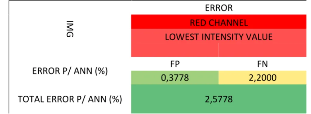
On Table 3.1 are presented the results of evaluating the red channel lowest pixel intensity by block feature without any specific image treatment. As it is shown

the FP error is very acceptable while the FN error is somewhat exaggerated. As-sessing this data the image needed to present less contrast and more brightness (Figure 3.5) to evidence the eyelashes from the red channel lowest pixel intensity by block“point of view”.

Table 3.1 - Results of red channel lowest pixel intensity before the brightness and contrast correction.

IMG ERROR

RED CHANNEL LOWEST INTENSITY VALUE

ERROR P/ ANN (%) FP FN

0,3778 2,2000

(44)

Figure 3.5 - Original image after brightness and contrast correction. (a) Original image after the contrast being de-creased; (b) Original image after the contrast being decreased and brightness being increased.

Table 3.2 -Results of red channel lowest pixel intensity after the brightness and contrast correction.

IMG ERROR

RED CHANNEL LOWEST INTENSITY VALUE

CONTRAST: -75%; BRIGHTNESS: 10%

0,4556 1,1000

TOTAL ERROR P/ ANN (%) 1,5556

The results in Table 3.2, after brightness and contrast correction, show an almost identical but slightly worse FP error when compared to the previous one, but the FN error demonstrate a great decrease which leads to a much acceptable

total error. These results validate the corrections made to the brightness and con-trast in the original image for obtaining the proper red channel lowest pixel intensity by block feature.

(45)

er-ror. Assessing this data the image needed to present less contrast and less bright-ness (Figure 3.6) to evidence the artifacts (eyebrows and eyelashes) and not evi-dence the clinical ROI.

Table 3.3 - Results of red channel pixel intensity before the brightness and contrast correction.

IMG ERROR

RED CHANNEL AVERAGE PIXEL INTENSITY

ERROR P/ ANN (%)

FP FN

0,8333 3,1889

TOTAL ER-ROR P/ ANN (%)

4,0222

Figure 3.6 - Original image after brightness and contrast correction. (a) Original image after the contrast being de-creased; (b) Original image after the contrast and brightness being decreased.

(46)

Table 3.4 - Results of red channel pixel intensity after the brightness and contrast correction.

IMG

ERROR

RED CHANNEL AVERAGE PIXEL INTENSITY

CONTRAST: -50%; BRIGHTNESS: -20%

ERROR P/ ANN FP FN

0,2778 2,7000

TOTAL ERROR P/ ANN 2,9778

In Table 3.5 are evaluated the first results of green channel pixel intensity by block feature without any specific image treatment. Here the FP error is too high while the FN error is very acceptable which leads to a high total error. Assessing this data the image needed to present a little less contrast and much less bright-ness (Figure 3.7) to be able to detect the artifacts (eyebrows and eyelashes).

Table 3.5 - Results of green channel pixel intensity before the brightness and contrast correction.

IMG

ERROR

GREEN CHANNEL AVERAGE PIXEL INTENSITY

ERROR P/ ANN (%)

FP FN

2,3778 0,8556

(47)

Figure 3.7 - Original image after brightness and contrast correction. (a) Original image after the contrast being slightly decreased; (b) Original image after the contrast and brightness being decreased.

The results in Table 3.6, after brightness and contrast correction, show a much improved FP error when compared to the previous one, before brightness and contrast correction, and a slightly increase in the FN error which, ultimately leads to a much more acceptable total error validating the corrections made to the brightness and contrast in the original image for obtaining the proper green channel pixel intensity by block feature.

Table 3.6 - Results of green channel pixel intensity after the brightness and contrast correction.

IMG ERROR

GREEN CHANNEL AVERAGE PIXEL INTENSITY

CONTRAST: -25%; BRIGHTNESS: -20%

ERROR P/ ANN (%)

FP FN

0,6222 1,7479

2,3701

(48)

Assessing this data the image needed to present much less contrast and more brightness (Figure 3.8) to not over detect the clinical ROI.

Table 3.7 - Results of magnitude FFT before the brightness and contrast correction.

IMG ERROR

FFT MAGNITUDE

ERROR P/

ANN (%)

FP FN

0,0778 7,8889

7,9667

Figure 3.8 - Original image after brightness and contrast correction. (a) Original image after the contrast being de-creased; (b) Original image after the contrast being decreased and brightness being increased.

The results in Table 3.8, after brightness and contrast correction, show an

increased FP error when compared to the previous one, before brightness and contrast correction, to compensate the extremely drop in the FN error which, ul-timately leads to a much more acceptable total error approving the corrections made to the brightness and contrast in the original image for obtaining the proper

(49)

Table 3.8 - Results of FFT magnitude after the brightness and contrast correction.

IMG

ERROR

FFT MAGNITUDE

CONTRAST: -75%; BRIGHTNESS: 0.7%

0,4778 2,5444

TOTAL ERROR P/ ANN (%) 3,0222

These results demonstrate the importance of the brightness and contrast correction throughout the characteristics in study as the total error have shown a decrement for all the specific image characteristics in study while maintaining the FP error, more important, virtually nil.

3.2.2 Image orientation

Before retrieving all the information necessary for image processing and as

the blocks’ location on the image have an important role as block feature, it is crucial to have all the images oriented similarly. The most common problem is that left and right eyes have the optic disk in opposite horizontal locations and for automatic image analysis this should be corrected. This step is then responsi-ble to orientate all images using the same final criteria.

(50)

In this work an image is considered correctly oriented when the optic disc is located on the right side of the image (Figure 3.9 (a)) and when it is inverted it is considered with an incorrect orientation. When the image has an incorrect

ori-entation a horizontal flip is necessary.

Figure 3.10 - Reversing the orientation of the image. (a) Original image; (b) Original image correctly inverted.

To automatically invert the image when it is necessary, the image is divided

(51)

Figure 3.11 - Region containing the optic disc; Image above in values; Image below in colors.

3.2.3 Gathering and preparation of the characteristics

(52)

Figure 3.12 - Image divided into 400 (20x20) small images.

Each of the 400 images is evaluated and from each one are acquired the distance to the center of the original image, the red channel pixel intensity (Figure 3.13), the red channel lowest pixel intensity, the green channel pixel intensity and the FFT magnitude.

Figure 3.13 - Red channel average pixel intensity values per block.

Since artificial neural networks have a better convergence when the inputs are in the [0…1] interval, the information is then normalized to this interval by dividing by the maximum feature value. The information is now fully prepared

(53)

3.3 Region Classification

In this stage the information is presented to previously trained automatic classifiers, capable of read the specific information previously treated, evaluate it and to provide a set of ROI’s as a response.

Figure 3.14 - Structure of the image processing phase and its methods.

For this works purpose it was empirically found that using an artificial neu-ral network (ANN) for each of the four specific characteristics (red channel pixel and lowest pixel intensity, green channel pixel intensity and FFT magnitude) pro-vides the best results for an automatic classification. All ANN had the same ge-ometry, all had four layers: one input layer, two hidden layers and one output

layer; the input and hidden layers were each composed by two neurons while the output layer were composed by one. The neurons of the input layer were responsible for receiving the information containing the distance of the block to the center of the image and the information regarding the specific characteristic feature of the ANN. The neurons corresponding to the hidden layers were re-sponsible for classifying the information and decide its direction. The neuron of the output layer were responsible for giving the result of that specific ANN and its result varied between 0 and 1 where a result close to 0 stood for a region of the image containing artifacts while a result close to 1 a region of the image that would be part of the clinical ROI (Heaton 2008).

All ANNs referenced above were trained with twelve images through the

back-propagation method. From those twelve images were gathered information of the specific characteristics of the image also by cropping the image into blocks. At each block were attributed the value of 0 or 1 according to the image there, if the image contained part of an artifact at that block were attributed the value 0 if

(54)

not at that block were attributed the value 1. Each ANN were trained by taking into account the value of judgment made.

Therefore, depending on the information entering the corresponding ANN

a value close to 0 or 1 leaves the ANN providing, in that way, the first ROI of the image. As there are four different ANNs, for each of the specific characteristics, after this phase there will be four different ROIs. To join all this information more processing is require as the next phase, image post-processing, will demonstrate.

3.4 Image Post-Processing

The main goal for this phase is to aggregate all the information into one final clinical ROI with the minimum error possible, and preferably with no

de-fault error at all. In this phase an image resulting from an OTSU binarization will be one additional information to aggregate with the ones already obtained. After all the information is computed, the final image presented to the user is prepared by darkening the regions containing artifacts.

Figure 3.15 - Structure of the image post-processing phase and its methods.

3.4.1 Image threshold

For this step a normal OTSU binarization (Otsu 1975) containing the 256 pixel intensities is applied.

APPLICATION OF AG-GREGATION

ALGO-RITHM

(55)

Figure 3.16 – Binarized image after OTSU Thresholding.

After the image is binarized the resulting image is cropped into 400 (20x20) blocks (Figure 3.16), just as for the specific characteristics. If the image in the block contains at least one pixel with zero intensity then this block is assigned the value 0 (contains artifacts) otherwise this block is assigned to the value 1 (part of the ROI).

3.4.2 Aggregation algorithm

After computing the five ROI required: red channel pixel intensity ROI, red channel lowest pixel intensity ROI, green channel pixel intensity ROI, the FFT magnitude ROI and the OTSU binarization ROI; the next step is to aggregate all of them into one single ROI.

(56)

Figure 3.17 – Resulting ROI of aggregation algorithm.

3.4.3 ROI final post-processing

Having a first tentative ROI the next step is to find and eliminate regions falsely selected as containing artifacts or being part of the ROI.

In this step all ROI matrix regions are re-analyzed following the rule: if the region contains artifacts and if there are at least three regions surrounding it (above, below, left and/or right) containing no artifacts then the region is corrected as containing no artifacts too otherwise the region remains the same (Figure 3.18). After the ROI matrix have been completely analyzed and the region values cor-rected, this new ROI matrix is re-analyzed again with an extra condition, to check if there is a region containing no artifacts completely surrounded by regions con-taining artifacts, if so then the region is corrected to containing artifacts. In this final rule if there is a region containing artifacts in the center of the image it will corre-spond to the macula area and then the region is corrected to containing no artifacts

(Figure 3.19).

(57)

Figure 3.19 - Final crossing resulting ROI.

3.4.4 Darkening of the regions containing artifacts

The next step is to darken the regions containing artifacts (the regions cor-responding to 0 in the final ROI). For that purpose a ROI matrix has been created

containing only the regions having artifacts.

Finally, the brightness is reduced on those ROIs remaining in the ROIs

ma-trix, thus creating a final image identical to the original one but with the regions containing artifacts darkened.

3.5 Summary

The presentation of the methodology for automatic delimitation of the clin-ical ROI in fundus images of the retina is now complete. As main methods in this methodology the aggregation algorithm and ROI final post-processing assume great importance.

The aggregation algorithm and ROI final post-processing altogether represent a new algorithm proposed in this work that showed to be a consistent way of post-processing the data with reliable results.

(58)

(59)

Chapter 4. Methods of Validation

In this chapter is presented the tool developed for validating the proposed methodology. It implemented all algorithms describe before. The main goal when implementing this software was to create the more user friendly graphical user interface (GUI) possible and so that no previous user training is required. This software is better suited for complementing automatic diagnosis and seg-mentation programs, as it simple to implement and can be easily attached to those programs.

Figure 4.1 - Graphical user interface (GUI) of the automatic delimitation of the clinical ROI software.

4

ORIGINAL IMAGE

(60)

Figure 4.1 shows the produced graphical interface. The resulting image will appear in the right, while the original image will remain on the left allowing a comparison between the two images and the results evaluation. To facilitate the

assessment if one region of the image has been correctly darkened or if there was a region left to be darkened, a grid can be overlaid to the image (Figure 4.2).

Figure 4.2 - Resulting image with the grid selected.

To validate the data an individual evaluation of each block in the resulting image is necessary, the results will be calculated after assessing each block of each

image if it has been properly evaluated.

For a better understanding of the program and all its functions a more de-tailed explanation is given in the following sections.

4.1 GUI

The full description of the GUI will be divided in its design and its func-tionalities, which will be presented next.

4.1.1 Design

(61)

 Two picture boxes, one for the original image and another for the resulting image;

 Two panels, one that shows all the images present in the working folder and another (history panel) that shows the images which al-ready have been analyzed;

 Main menu containing three items:

o _{File containing four menu items: Open Image; Open Folder;}

Save Image; Exit;

o _{Edit containing an Undo menu item;}

o _{ROI containing a Final menu item.}

 Grid button to show or remove the grid from the resulting image.

 Set of buttons to select how to see the original image: red channel, green channel, both images, image with both channels (original

im-age) or the three images.

Figure 4.3 - Detailed GUI.

4.1.2 Functionalities

Before being ready to execute the program it is important to know the

func-tions that aren’t very explicit.

The Open menu item in the FILE menu opens a single image appearing in

the original image picture box, instead the Open Folder menu item opens all images in a folder selected by the user and displays them in the Folder Images Panel. In

ORIGINAL IMAGE RESULTING IMAGE

(62)

this latter option if the user from the folder panel selects one image, it appears in the original image picture box. The Save As menu item in the FILE menu saves the image in the resulting image picture box with a name and file extension chosen by

the user. The Undo item in the EDIT menu places the previous image in the orig-inal image picture box.

When a new image is sent to the resulting image picture box, the previous image is sent to the history panel. All images in the history panel can be assessed by clicking on them, appearing in the resulting image picture box.

By clicking on Final menu item in the ROI menu the image in the original image picture box will be processed and the its final ROI will be presented in the

resulting image picture box with, approximately, one minute time delay.

Important note

To allow for the ROI menu function a primary evaluation had to be made before for studying purposes. As the original image were cropped into blocks a

table and the image cropped would appeared below the original image picture box

with the possibility of a value or color visualization of each image feature (Figure 4.4) and if a block was selected a list of its entire features were presented (Figure 4.5).

(63)

Figure 4.5 – Features list of the selected image block.

4.2 Summary

The software created achieved the objectives, as not only the program is user-friendly but also works as a validation method for the automatic clinical ROI delimitation. The program has few objects and each one has a tooltip with indications of what purpose it serves.

(64)

(65)

Chapter 5. Results Evaluation

The results evaluation and the assessment of their efficiency was held by comparing the final clinical ROI with the expected one, checking block by block if the area has been correctly darkened. With the individual data of each image available, predictive values and statistical values, such as specificity and sensi-tivity, have been calculated.

In this work the specificity, the ability of a test to correctly classify the neg-atives, has more importance than the sensitivity, the ability of a test to correctly classify the positives, as such, a final table with those indicators is needed for a combined final assessment.

5.1 Materials and Methods

The images used to assess the accuracy of the automatic delimitation method were obtain from a fundus images database. The validity of the results were measured using a set of statistical measures, such as specificity and sensi-tivity.

5.1.1 Images Database

A set of 43 retinal fundus images from OPTOS color fundus image library

(66)

taken by an OPTOMAP machine which allowed an approximately 200º fundus image of the retina. The dataset contains images correctly acquired and images containing malfunctions or a strong amount of artifacts. Each fundus image has

the normal features of an OPTOMAP image, i.e., information only on red and green channels and each one with 256 intensity levels. No modification, to adapt or improve the images was necessary for the program to work.

5.1.2 Methods

The results evaluation were performed by comparing the resulting image with the original image having the artifacts marked by a specialized person. The assessment was done comparing block by block and one block could fall into one of four testing results: True Positive(TP) if the block were correctly selected as part of the clinical ROI; True Negative (TN) if the block were correctly selected as not partof the clinical ROI; FalsePositive(FP) if a block were incorrectly selected as part of the clinical ROI; False Negative (FN) if a block were incorrectly selected as not partof the clinical ROI;

For the comparative analysis indicators such as sensitivity, specificity, pre-cision, accuracy and false negative rate were calculated.

Finally, to assess a final error, a cost matrix with weights, were performed to unite the values of false negative error and false positive error into one.

5.1.2.1 Sensitivity, Specificity

In this work, sensitivity represents the proportion of the positives of the image that have been correctly evaluated as such and can be calculated using the formula below.

𝑠𝑒𝑛𝑠𝑖𝑡𝑖𝑣𝑖𝑡𝑦 = 𝑇𝑃 𝐹𝑁 + 𝑇𝑃⁄

On the other hand, specificity represents the proportion of the negatives of the image that have been correctly evaluated as such and can be calculated using the formula below.

(67)

Both specificity and sensitivity can vary between 0 and 100%, where a result close to 0% will stand for a low value and a result close to 100% for a high pro-gram.

5.1.2.2 Negative and Positive Predictive Values

The negative predictive value (PPV) represents the amount of tests consid-ered negatives that were in fact true negatives and can be calculated using the following formula.

𝑁𝑃𝑉 = 𝑇𝑁 𝐹𝑁 + 𝑇𝑁⁄

The positive predictive value (NPV) represents the amount of tests consid-ered positives that were, in fact, true positives and can be calculated using the following formula.

𝑃𝑃𝑉 = 𝑇𝑃 𝐹𝑃 + 𝑇𝑃⁄

In this work, both NPV and PPV, will describe its performance. A result close to 100% of those values will stand for a precise program.

5.1.2.3 Accuracy and Precision

In this work accuracy represents a degree of closeness of the result obtained to the true and known value. It can be calculated using the following formula.

𝑎𝑐𝑐𝑢𝑟𝑎𝑐𝑦 = 𝑇𝑃 + 𝑇𝑁 𝑃 + 𝑁⁄

On the other hand, precision represents a degree of closeness of two or more

results to each other and can be calculated with the formula below.

𝑝𝑟𝑒𝑐𝑖𝑠𝑖𝑜𝑛 = 𝑇𝑃 𝐹𝑃 + 𝑇𝑃⁄

A precision result close to 100% will stand for a program which, under the same conditions, will show the same results while a accuracy result close to 100% will stand for a program whose results are very close to the real and expected

(68)

5.2 Results

5.2.1 Sensitivity and Specificity Analysis

The sensitivity and specificity per image were calculated (Figure 5.1) as well the mean for both values (Table 5.1).

Figure 5.1 - Graphics of Sensitivity and Specificity per Image.

Table 5.1 - Mean Sensitivity and Specificity.

SENSTIIVITY SPECIFICITY

Mean

(69)

5.2.2 Negative and Positive Predictive Values

The NPV and PPV per image were calculated (Figure 5.2) as well the mean for both values (Table 5.2).

Figure 5.2 - Graphics of NPV and PPV per Image.

Table 5.2 - Mean PPV and NPV.

POSITIVE PREDICTIVE

VALUE

NEGATIVE PREDICTIVE

VALUE

Mean Value

(70)

5.2.3 Accuracy and Precision

The accuracy and precision per image were calculated (Figure 5.3) as well the mean for both values (Table 5.3).

Figure 5.3 - Graphics of Accuracy and Precision per Image.

Table 5.3 - Mean Accuracy and Precision.

ACCURACY PRECISION

Mean

(71)

5.2.4 Cost Matrix

Figure 5.4 - Graphics of FP and FN per image.

Table 5.4 - Mean FP and FN.

FP FN

Mean

Value (%) 0,0930 1,1512

Table 5.5 - Cost Matrix for FP and FN.

FN FP

FN 0 100

FP 40 0

(72)

5.3 Summary

This results can be considered good as they validate the automatic delimi-tation of the clinical ROI in retinal fundus images program.

The program can be considered accurate and precise as the results close to 100% (accuracy - 98,8%, precision - 99,7%) of both values demonstrate, even so the precision values are slightly better than the accuracy values which means that this program, under the same conditions, will present always excellent results that are very similar to the actual ones.

With values of NPV and PPV of 99,7% and 98,1% respectively, the precision assessment can be elaborated as both the “positive values precision” and

“nega-tive values precision”, PPV and NPV respec“nega-tively, are very good standing then

for a very good precision as well, still it can be said that the program is more precise for positive values as the values demonstrate.

Finally, and more important, assessing the specificity and sensitivity values it can be seen an almost perfect specificity (99,9%), which in this work stands for an almost perfect ability to correctly find the negative zones, zones with artifacts, in the image whereas for the sensitivity the values are slightly worse (96,9%), corresponding then for a slightly worse ability for the program to correctly find positive zones, zones corresponding for the clinical ROI, in the image.

(73)

(74)

(75)

Chapter 6. Conclusion

This thesis presented a full methodology for automatic delimitation of the clinical ROI in fundus images of the retina. By using digital imaging processing techniques a user independent program was developed, which allows a more objective criteria for automatic delimitation of the ROI in retinal fundus images.

Ultimately, supplying a tool for automatic disease diagnosis and automatic vessel segmentation programs that can reduce their false positives may prove to be very important. As the clinical ROI area in the resulting image is exactly as the same as that area in the original image, those automatic programs need no pre-vious or extra treatment for them to properly work. Thus, the existence of a tool that can be incorporated into software with the advantage of instantly improve its performance, may reveal to be of great importance.

Having an algorithm that does not require user intervention not only im-prove its accuracy and repeatability, but also proportionate the use of less human resources and also accelerates the process, which, eventually, end up improving the patients quality of life.

Ricardo Jorge Guerreiro Antunes

Automatic delimitation of the clinical region of

interest in ultra-wide field of view images of the

retina

A

Acknowledgements

Table of Contents

-List of Tables

Acronyms

Chapter 1.

Introduction

1.1

Human Eye

1.2

Retina

1.3

Ultra-Wide Field Scanning Laser Ophthalmoscopy (OPTOMAP)

1.4

Important Retinal Diseases

1.5

What is proposed in this thesis?

1.6

Thesis structure

Chapter 2.

Literature Review

2.1

Segmenting Eyelids

2.2

Segmenting Eyelashes

2.3

Segmenting eyelids and eyelashes in OPTOMAP

2.4

Discussion

Chapter 3.

Methods of Detection

3.1

The Methodology

3.2

Image Processing

3.3

Region Classification

3.4

Image Post-Processing

3.5

Summary

Chapter 4.

Methods of Validation

4

4.1

GUI

4.2

Summary

Chapter 5.

Results Evaluation

5.1

Materials and Methods

5.1.2.1

Sensitivity, Specificity

5.1.2.2

Negative and Positive Predictive Values

5.1.2.3

Accuracy and Precision

5.2

Results

5.3

Summary

Chapter 6.

Conclusion