ESSAYS ON SUBJECTIVE WELL-BEING

(1)

ESSAYS ON SUBJECTIVE WELL-BEING

A Ph.D. Dissertation

by

TUGBA ZEYDANLI

European Doctorate in Economics Erasmus Mundus (EDE-EM)

Paris School of Economics, Universit`e Paris I:

Panth`eon-Sorbonne

Nova School of Business and Economics, Universidade Nova de

Lisboa

(2)

(3)

ABSTRACT

ESSAYS ON SUBJECTIVE WELL-BEING

ZEYDANLI, Tugba

Ph.D., Department of Economics

Supervisor: Prof. Dr. Jean-Marc Bonnisseau

Supervisor: Assoc. Prof. Dr. Pedro Vicente

May 2015

This dissertation consists of three essays on subjective well-being.

The first essay examines whether aggregate job satisfaction in a certain labor

market environment can have an impact on individual-level job satisfaction.

We seek an answer to this question using two different datasets from the United

Kingdom characterizing two different labor market environments: Workplace

Employment Relations Survey (WERS) at the workplace level (i.e., narrowly

defined worker groups) and British Household Panel Survey (BHPS) at the

local labor market level (i.e., larger worker groups defined in industry×region cells). Implementing an original empirical strategy to identify spillover effects,

we find that one standard deviation increase in aggregate job satisfaction leads

to a 0.42 standard deviation increase in individual-level job satisfaction at the

workplace level and 0.15 standard deviation increase in individual-level job

(4)

are sizable and should not be ignored in assessing the effectiveness of the

policies designed to improve job satisfaction.

Individuals tend to self-report higher subjective well-being levels on certain

days of the weeks than they do on the remaining days, controlling for observed

variation. The second essay tests whether this empirical observation suffers

from selection bias by using the 2008 release of the British Household Panel

Survey. In other words, we examine if subjective well-being is correlated with

unobserved characteristics that lead the individuals to take the interview on

specific days of the week. We focus on two distinct well-being measures: job

satisfaction and happiness. We provide convincing evidence for both of these

measures that the interviews are not randomly distributed across the days of

the week. In other words, individuals with certain unobserved characteristics

tend to take the interviews selectively. We conclude that a considerable part

of the day-of-the-week patterns can be explained by a standard “non-random

sorting on unobservables” argument rather than “mood fluctuations”. This

means that the day-of-the-week estimates reported in the literature are likely

to be biased and should be treated cautiously.

In Sub-Saharan Africa, some scholars identify ethnicity as a cause of

instabil-ity and poor economic growth, which is due to worse public policies. Eifert, Miguel, and Posner (2010) show that ethnic identification is more prominent during competitive election periods in comparison to other identifying

cate-gories such as gender, religion, and class/occupation. The third essay utilizes

(5)

from the Afrobarometer. It asks if individual subjective well-being changes in

the run up to competitive elections. We find strong evidence that individual

subjective well-being does change. It is positively related to the proximity to

an election and this proximity effect depends on the competitiveness of the

election. We further investigate the background mechanisms behind this

posi-tive relationship i.e.: to what extent does well-being of the individual change if

the party that the individual supports wins the election, and is there a change

in well-being of the individual before and after the election? In addition, we

document that ethnic identification also has a positive impact on individual

well-being after controlling for electoral cycle variables. Policy makers should

internalize these positive externalities driven from politically-induced ethnic

identification.

JEL codes: C25, C31, D60, D62, I31, J28, O55, O15.

Keywords: Subjective well-being; social interactions; spillovers; hierarchical

model; day-of-the-week effects; self-selection; treatment effects; ethnicity;

(6)

ACKNOWLEDGEMENTS

First and foremost I offer my sincerest gratitude to my supervisors, Jean-Marc

Bonnisseau and Pedro Vicente, who have supported me throughout my thesis

with their patience and knowledge while allowing me the room to work in my

own way. I am also indebted to my co-authors; Semih Tumen and Alexander

Hijzen, who gave their time and provided worthy guidance. I am also indebted

to Andrew Clark and Claudia Senik for their insightful comments throughout

my thesis study. I would like to thank Olivier Bargain and Roxana

Guti´errez-Romero, who are the examining committee members, and provided detailed

helpful comments and suggestions on my thesis. I also would like to thank

and Louis L´evy-Garboua and Ana Balcao Reis for very helpful comments, and

constructive attitude.

I would like to thank European Doctorate in Economics – Erasmus Mundus

(EDE-EM) for its financial support during my study. I also would like to thank

to administrative office of both universities and the EDE-EM.

Special thanks to my graduate friends for their generous help, invaluable smile

and close friendship. Life would have been just too tedious without delighted

(7)

support. I cannot ask for more from my family, as they are perfect. I am

waking up to a world where I am simply happy.

However, while grateful to them, I bear the sole responsibilities for all the

(8)

LIST OF TABLES

2.1 Summary Statistics—WERS . . . 61

2.2 Summary Statistics—BHPS . . . 62

2.3 Summary Statistics—Job Satisfaction score over re-gion . . . 63

2.4 Estimation results—WERS. . . 64

2.5 Estimation results—BHPS . . . 65

2.6 Group-level interaction terms—WERS . . . 66

2.7 Linear-in-means model—WERS . . . 67

2.8 π=0—WERS . . . 68

2.9 Group means exclude i—WERS . . . 69

2.10 Group means exclude i, firm fixed effects included—WERS . . . 70

2.11 Group means exclude i, industry-region cell fixed effects in-cluded—BHPS . . . 71

2.12 Job Satisfaction Score (7-35)—WERS . . . 72

2.13 Aggregation of Job Satisfaction Components—WERS 73 2.14 Aggregation of Job Satisfaction Components—BHPS 74 2.15 Industry × Region—WERS . . . 75

(12)

3.1 Summary statistics—BHPS (1992-2009) . . . 103

3.2 Day orderings . . . 104

3.3 Bunching the days . . . 105

3.4 Day patterns conditional on observed variation. . . . 107

3.5 Probit regression. . . 108

3.6 Second step (job satisfaction). . . 109

3.7 Second step (happiness) . . . 110

3.8 Estimated treatment effects . . . 111

3.9 Estimated treatment effects for education categories112 3.10 Estimated treatment effects for sub-groups . . . 113

4.1 Summary Statistics-Afrobarometer, Round 1-2-3-4 . . 142

4.2 Economic and Political Characteristics of Countries143 4.3.1Your Living Conditions and Electoral Cycle . . . 145

4.3.2Your Living Conditions Compared to Others and Elec-toral Cycle . . . 145

4.3.3Mental Health and Electoral Cycle . . . 146

4.4 Personal Identification and Subjective Well-Being . 146 4.5 The Salience of Ethnic Identification . . . 147

4.6.1Before the election . . . 148

4.6.2Public Expenditures . . . 149

4.6.3Winning the election . . . 149

4.6.4Interested in Public Affairs . . . 150

4.6.5Illegitimacy of Elections . . . 150

(13)

LIST OF FIGURES

3.1 Interviewer ID (job satisfaction) . . . 106 3.2 Interviewer ID (happiness) . . . 106 3.3 Treatment effects by age categories (job

satisfac-tion). . . 114 3.4 Treatment effects by age categories (happiness). . . 114 4.1 Electoral Proximity and Subjective Well-Being, by

(14)

CHAPTER 1 INTRODUCTION

For such a long time, economists have ignored researching individual subjective

well-being. They left the study of happiness to other disciplines, especially

psychology. When the science of economics was founded by the classics, they

thought that happiness can be measured and used to determine whether a

particular economic policy raises or lowers the happiness of the people affected.

Thereby, Jeremy Bentham for instance assumed that utility reflects pleasures

and pains, and Isidor Edgeworth believed that happiness can be measured by a

hedonometer. The situation started to change with the normative economics

that what the outcome of the public policy ought to be. It was followed

by “New Welfare Economics”, which was a normative branch of economics.

John Hicks demonstrated that human behavior, and in particular, the demand

for commodities can be explained on the basis of relative utility. Welfare

judgements can be made by resorting to the Pareto criterion, and therefore,

no comparison of welfare levels among individuals is required. This approach

(15)

However, today there is a dramatical change in economists’ thinking.

Psychol-ogists have launched new ways of measuring utility [Kahneman, Diener, and Schwarz (1999)]. One way makes it possible to approximate individual util-ity in a satisfactory way by posing one question—or a combination of several

question— in representative surveys. This question enables researchers to

ob-tain indications of individuals’ evaluations of their life satisfaction/happiness.

In general, as in the literature, the terms “happiness”, “well-being”, and “life

satisfaction” are used interchangeably.

Moreover, there is a vast literature that proves that the measures of reported

subjective well-being can serve as a proxy for individual utility. From then

onwards, there has been steadily increasing research in subjective well-being

on the side of economists. Subjective well-being research adds a considerable

number of new insights to well-known theoretical proportions. However, it

is still debatable to what extent these “traditional” measures of subjective

well-being accurately capture the various notions of individual utility. On the

other hand, subjective well-being enables testing different aspects of life-events

which could not be solved with using revealed preferences.

This dissertation consists of three essays on subjective well-being. The first and

the third essay address the new possibilities offered by subjective well-being.

The first one tries to understand whether individual subjective well-being can

change with social interactions and the third one analyzes the relationship

between personal identities such as ethnicity and political competition from a

(16)

trust subjective well-being data given it’s subject to “mood fluctuations”.

More specifically, in order to analyze labor market phenomena, the first essay

makes use of job satisfaction data with an interest on social interaction by

utilizing the British Household Panel Survey Data (BHPS)1

and the

Work-place Employment Relations Survey (WERS)2

. The second essay investigates

whether the day-of-the-week effect estimates reported in the empirical

sub-jective well-being literature suffer from selectivity bias in large panel dataset

(BHPS). Finally, the last essay investigates subjective well-being in the

frame-work of political and development economics. It examines the impact of

com-petitive elections and ethnic identification on subjective well-being in

Sub-Saharan Africa.

The following subsections give brief description about chapters, and outline

the thesis.

1.1 Social Interactions in Job Satisfaction

In most research, job satisfaction is documented as being positively correlated

with worker performance and productivity. But whether there are any visible

footprints of social interactions in job satisfaction or not is an unanswered

question. How do my colleagues job satisfaction levels in the workplace affect

mine? To what extent does the job satisfaction of people with whom I am

1

The BHPS provides information on individual, household, and job/employer-related characteristics from 1991 to 2008 in England, Scotland, Wales, and Northern Ireland.

2

(17)

working within the same industry and region influence my job satisfaction?

What kind of group-level interactions can affect my job satisfaction level?

An-swers to these questions may be important for designing policies to increase

job satisfaction. Overall, this study examines whether aggregate job

satis-faction level in a certain labour market environment can have an impact on

individual-level job satisfaction. If the answer is yes, then policies aimed to

increase job satisfaction can increase productivity through social interactions

as well.

This study conducts the analysis at two aggregation levels using two

differ-ent datasets from the UK. First, the 2004 Workplace Employmdiffer-ent Relations

Survey (WERS) is to test the existence of job satisfaction spillovers at the

workplace level. In the workplace-level analysis, the reference group that the

social forces are effective is the set of workers in each workplace. Second, the

2004 British Household Panel Survey (BHPS) is to form industry-region cells

for the purpose of testing the existence of spillovers at the local labour

mar-ket level. The second exercise tries to capture social processes that involve

collective aspects of community and work life. The conclusion of the paper is

that there are sizable social interactions in job satisfaction that should not be

ignored in assessing policy effectiveness.

An increase in aggregate job satisfaction level leads to three times higher

in-crease in individual-level job satisfaction at the workplace than at the local

labour market. Contextual social effects also have a significant impact on

(18)

individual-level goes up when a larger fraction of male and older workers are

present. At the local labour market level, the findings say that individual-level

job satisfaction score goes down as the fraction of workers with greater access

to promotion opportunities goes up in each industry-region cell. There are

significant income-comparison effects at the workplace, but not at the local

labour market. In particular, individual-level job satisfaction goes down with

average earnings and the fraction of high earners that is, those who earn above

the median wage within the relevant worker population in the workplace.

These results suggest first, that there are large gains to policy interventions

to increase individual-level job satisfaction, as there are significant positive

feedback effects from group-level job satisfaction toward individual-level job

satisfaction in the form of spillover externalities. Second, failing to account

for the spillover externalities in job satisfaction may lead to an incorrect

as-sessment of the effectiveness of job satisfaction policies. Thus, policy-makers

should internalise these externalities. Third, job satisfaction spillovers are

much stronger at the workplace level than local labour market level: therefore,

designing and enforcing job satisfaction policies at the workplace level will

likely be more effective than implementing such policies at the local labour

market level.

1.2 Selection Correction on Day-Of-The-Week

Empirical studies document that individuals tend to report lower levels of

(19)

satisfaction levels on Fridays and/or Saturdays than the other days of the week,

controlling for observed variation [Taylor(2006),Akay and Martinsson(2009), and Helliwell and Wang (2013)]. These results are based on the main micro-level datasets such as the British Household Panel Survey (BHPS), the German

Socio-Economic Panel Survey (GSOEP), and the Gallup/Healthways polls as

well as several small-scale surveys. This literature suggests that subjective

well-being varies significantly across the days of the week.

Are people’s mood really sensitive to the day-of-the-week or do people actually

select the day-of-the-week that they take the survey depend on their daily

routine and/or their unobserved characteristics? As an example, self reported

job satisfaction is the highest on Fridays and Saturdays, it may be the case

that hard-working individuals —already highly satisfied jobwise— have only

time left to fill the survey on days like Friday or Saturdays since they are

occupied with work during the week. Alternatively, individuals, who are not

working hard throughout the week can prefer to take the survey on Sundays

instead of resting or Monday, which can be a good reason for procrastination

due to the overload go beginning of new week. These types of individuals can

be already unsatisfied with their jobs or lives in general. Overall, if selectivity

is in action, then this would weaken the argument of “mood” fluctuations over

the days of the week.

To summarize, the main hypothesis we test in this essay is: the

day-of-the-week estimates reported in the empirical literature may be contaminated with

(20)

for economic modeling. If the selection bias is significant and, as a result,

the day-of-the-week effects disappear after selection correction, then this will

cast doubt on the relevance of the “mood fluctuations” argument. Thus, the

shadow hypothesis we test is the relevance of the “neoclassical stable

prefer-ences assumption” against preferprefer-ences subject to “mood fluctuations”.

This study finds significant positive selection both for job satisfaction and

hap-piness, utilizing the 2008 release of British Household Panel Survey (BHPS).

For job satisfaction, the ones who are interviewed on Fridays or Saturdays tend

to report higher job satisfaction and for happiness, those who are interviewed

on Sundays or Mondays tend to report lower happiness levels than a random

sample drawn from the population of employed workers with a comparable set

of observed characteristic would report. The conclusion of the paper is that

the magnitude of the selection bias originating from these compositional shifts

is so large that there is only little room for the “mood fluctuations” argument.

After selection correction, the estimated treatment effects for job satisfaction

are higher among males, non-married workers, workers with permanent jobs,

public sector workers, workers in large firms, union members, workers with

good health, workers who prefer to work less, workers with higher relative

in-come, workers with higher education, and middle-aged workers. The patterns

are similar for happiness as well.

These findings provide evidence that the existence of weekly cycles in

individ-ual subjective well-being may not be as relevant as the literature documents.

(21)

determin-ing well-bedetermin-ing scores, and the compositional changes in interviewees in terms

of these heterogeneous factors drive most of the observed differences is

self-reported subjective well-being across the days of the week.

We do not totally rule out the state-dependent nature of utility. Utility may

be changing across states if these states reflect some fundamental feature of

individual utility; such as employment status, marital status, etc. We rather

argue that day-to-day shifts in agents’ valuation of economic objects do not

have strong empirical basis, when selectivity is controlled for.

1.3 Competitive Elections and Ethnic

Identi-fication

Ethnic identity in Africa is formed the individual’s life settings. The relevance

of ethnic identification is controversial; some scholars argue that the source

is culture, and for others is politics. Recently Eifert, Miguel, and Posner (2010) stated, the source of ethnic salience comes from political competition: in other words, proximity to competitive elections increases the strength of

ethnic attachments.

In ethnically diverse countries, political parties have used ethnic identity to

mobilize voters and to establish political alliances, leading in some cases to

violent ethnic conflicts. In competitive elections this can result in the loss

(22)

heterogeneity and slow growth in Sub-Saharan Africa (SSA). Some scholars

point out ethnicity as a cause of instability and poor economic growth, which

is due to worse public policies.

This study poses the following questions “How does the competitive election

affect happiness of the people?”, “Does a competitive election make them

hap-pier than a landslide election?”, “If a competitive election makes the people

happier, what is the underlying mechanism?, and “How happy are the

peo-ple if they identify themselves ethnically?” Answering these questions may be

important for policies as opposed to politically-induced ethnic identification.

Overall, the first aim of the study is to determine how competitive elections

affect the individual subjective well-being when they are proximate. As the

second aim, since competitive elections increase the salience of ethnic

identi-fication, this study investigates the relationship between ethnic identification

and subjective well-being after controlling for electoral cycle variables.

We conduct the analysis with several well-being questions, which the

Afro-barometer includes, across 12 African countries over 40,000 respondents. The

results show that for every month closer a country is to a competitive election,

on average individual-level subjective well-being has a 0.015 standard

devi-ation increase. There are several possible mechanisms that account for this

positive relationship. The more prominent ones are winning the election;

sub-jective well-being of the individual gets positively stronger if the party that the

individual support wins the competitive election, and the asymmetrical effects

(23)

related to subjective well-being, but the impact before the election is greater

than that after the election. The result of the second aim is that if individuals

identify themselves ethnically, this is positively correlated with individual-level

subjective well-being after controlling for electoral cycle variables.

These findings suggest that positive externalities exists from competitive

elec-tions and ethnic identification to the individual subjective well-being. These

results should be taken into consideration when implementing policies opposed

to politically induced ethnic identification. Ethnicity can help to develop

so-ciety, both socially and economically, by mobilizing people to initiate

develop-ment projects in their communities. However, one should be cautious about

that these findings are only affected in short-term, the effects of long-term are

unknown.

1.4 Thesis Outline

Chapter 2 examines whether there is any visible footprints of social interaction

in job satisfaction by utilizing two different dataset and social environment.

Chapter 3 first replicates the literature findings about relationship between

subjective well-being and days-of-the-week and then asks if these

day-of-the-week estimates for job satisfaction and happiness measures suffer from selection

bias in large panel dataset. Chapter 4 investigates how competitive elections

affect individual subjective well-being when they are proximate and how the

ethnic identification is related to subjective well-being.

(24)

work of Chapter 2 [Tumen and Zeydanli (2014)] is forthcoming at Journal of Happiness Studies. Chapter 3 is forthcoming at Social Indicators Research.

The ideas contained in this thesis aim at contributing subjective well-being

literature and shall not be associated with views of any of the aforementioned

institutions nor their policies. Any errors are mine.

Each chapter is a self-contained manuscript. For the reader’s convenience, the

(25)

CHAPTER 2 SOCIAL INTERACTION IN JOB

SATISFACTION

Job satisfaction is a direct measure of utility an employed worker derives from

his/her current job [Clark and Oswald (1996)]. It has extensive behavioral consequences. For example, job satisfaction is a significant determinant of

la-bor market mobility—in particular, the quitting behavior.1

It is also shown

to be related to relative pay comparisons among peer groups in the

work-place.2

Most importantly, and this is mainly why labor economists should be

interested in job satisfaction, it is documented to have a positive correlation

with labor productivity and worker performance.3

In particular, Boeckerman and Ilmakunnas (2012) document that job satisfaction has a causal effect on productivity.4

To get the feel of the magnitude, Boeckerman and Ilmakunnas 1

See, e.g.,Freeman(1978),Akerlof et al.(1988),Clark et al.(1998), andClark(2001). 2

See, for example,Clark et al.(2009) andCard et al.(2012). 3

Other studies documenting this positive relationship include, but are not limited to,

Iaffaldano and Muchinsky(1985), Ostroff (1992), Brown and Peterson (1994),Ryan et al.

(1996),Sloane and Williams(2000),Argyle(2001),Judge et al.(2001),Harter et al.(2002),

Schneider et al. (2003), Patterson et al. (2004), Green and Tsitsianis (2005), Otis and Pelletier(2005),Christen et al.(2006),Ghinetti (2007), andWegge et al. (2007). Zelenski et al. (2008) and Oswald et al. (2014) argue that happiness and life satisfaction are also positively correlated with productivity.

4

(26)

(2012) find that one standard deviation increase in job satisfaction within the plant increases productivity per hours worked by 6.6 percent.

Although several aspects of job satisfaction have been studied extensively in

the empirical literature, whether there exist spillover externalities in job

satis-faction—i.e., whether individual-level job satisfaction is affected by the

aggre-gate job satisfaction in a certain labor market environment—or not remains

as an unanswered question. This is a relevant question because job

satisfac-tion is often associated with workplace attitudes such as involvement in the

organization, relatedness with co-workers/customers/managers, attachment,

motivation, shirking, tendency to slow down work, absenteeism, etc. These

attitudes form a workplace “atmosphere” and jointly contribute to the

for-mation of worker satisfaction and performance. Therefore, the aggregate job

satisfaction level in a certain work environment can be regarded as a “social”

variable and may, in turn, affect individual-level job satisfaction.

Our ultimate goal in this paper is to investigate if there exist any visible

foot-prints of social interactions in job satisfaction. Answering this question is

also important for policy. If there exist positive spillovers in job satisfaction,

then policies targeted to increase job satisfaction can boost productivity not

only directly, but through spillover externalities too. When these social

inter-actions effects are sizable, ignoring them may lead to mis-assessment of the

effectiveness of the policies designed to improve job satisfaction in various work

environments.

(27)

We perform our empirical analysis at two aggregation levels using two different

data sets from the United Kingdom. First, we use the Workplace Employment

Relations Survey (WERS) to test the existence of job satisfaction spillovers at

the workplace level (or establishment-level).5

In the workplace-level analysis,

the reference group that the social forces are effective is the set of workers in

each workplace. Second, we use the British Household Panel Survey (BHPS) to

form industry_×region cells for the purpose of testing the existence of spillovers at the local labor market level. In this second exercise, we try to capture more

general social effects in larger reference groups. The main purpose is to focus on

social processes that involve collective aspects of community and work life. In

both of these exercises, we concentrate on estimating the correlation between

the group-level and individual-level job satisfaction scores, controlling for a

large set of observed covariates. Drawing a distinction between the workplace

and local labor market level analyses is useful, because it will allow us to make

precise statements on whether it is more effective to enforce job satisfaction

policies at the establishment level (i.e., as firm-specific policies) or local labor

market level (i.e., in the form of broader institutional measures).

Our econometric framework will be a version of the canonical linear-in-means

model, which is a base for the bulk of empirical work on social interactions.6

The main problem with the linear-in-means model is that it necessitates

em-ploying a carefully-designed identification strategy to separate endogenous

ef-5

The terms “workplace” and “establishment” will be used interchangeably throughout the paper.

6

See Blume et al. (2011) for an in-depth background information on linear-in-means models, including a comprehensive discussion on micro-foundations and econometric iden-tification. Also seeBlume and Durlauf (2001), Brock and Durlauf(2001b), andSoetevent

(28)

fects from the contextual effects [Manski (1993)]. It will perhaps be useful at this point to clearly define the terms “endogenous social effects” and

“contex-tual social effects.”7

The endogenous effect refers to the effect of the

group-level outcome on the individual-group-level outcome. Within the context of our

paper, this corresponds to the effect of the group-level mean of job satisfaction

on the individual-level job satisfaction. The contextual effect, on the other

hand, refers to the effect of the group-level counterparts of the individual-level

observables on the individual-level outcome variable; in our paper, this

corre-sponds to the effect of, say, group-level average age or average education on

the individual-level job satisfaction score.

At the center of our identification strategy lies an insight from the

hierarchi-cal (or multilevel) statistihierarchi-cal models of social processes: social groups describe

“ecologies” in which decisions are made and matter because different ecologies

induce different mappings from the individual determinants of these decisions

to the associated outcomes [Raudenbush and Sampson(1999)]. Based on this conceptualization, we construct an empirical model in which contextual effects

(i.e., the “ecologies” in our model) alter the coefficients linking individual

char-acteristics to outcomes. This corresponds to allowing for multiplicative

inter-actions between the contextual effects and the remaining explanatory terms

within the linear-in-means model. We formally show that introducing these

cross-product terms induces non-linearities that resolve the reflection problem

Manski(1993) describes [see Section 2.3]. Such a setup secures the economet-ric identification of social interactions and enables us to separate endogenous

7

(29)

effects from the contextual effects [Blume and Durlauf (2005)]. Although, this approach is rather simple and intuitive, it is surprisingly under-utilized in the

literature.

There are two more potential threats to identification. The first one is the

possibility of sorting into reference groups based on unobserved factors [ Man-ski (1993)]. The sorting can be conducted two ways; one is via group-level unobserved factors and the other is via sorting into reference groups. These

two can also be potentially related to each other. If group-level unobserved

factors that determine individual-level job satisfaction exist and are also

cor-related with group-level job satisfaction, then the resulting estimates would

be biased. Our empirical approach also allows us to address this problem, at

least partially, by controlling for group-level unobservables in various ways.

Endogenous sorting would occur in several dimensions. It may be the case

that group-level unobserved factors trigger the selection but do not determine

the individual-level satisfaction. This relationship can also work inversely, i.e.,

group-level unobserved factors may be more recent than the sorting. However,

there are several limitations in solving endogenous group selection that we will

discuss later. And, second, it is well-documented in the literature that the

rel-ative income structure within the reference group is an important determinant

of the job satisfaction level in the peer group [Card et al. (2012)]. We also control for the pay-comparison effects in our calculations.

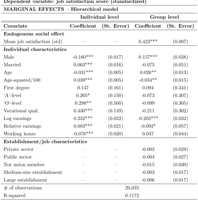
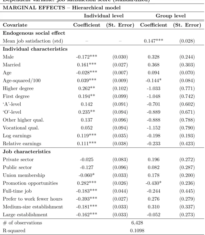
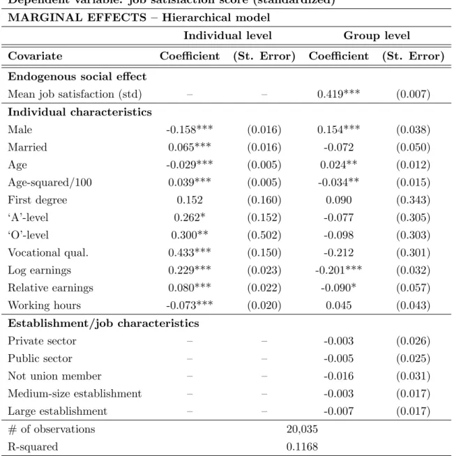
We find that one standard deviation increase in aggregate job satisfaction

(30)

satis-faction score at the workplace level and a 0.15 standard deviation increase in

individual-level job satisfaction score at the local labor market level. In other

words, we report that statistically significant job satisfaction spillovers exist

both at the establishment level and local labor market level; and, the estimated

spillovers are approximately three times larger at the establishment level than

those at the local labor market level. These estimates can be restated in terms

of the social multiplier: the corresponding social multipliers are [1/(1 - 0.42)_≈] 1.72 and [1/(1 - 0.15)≈] 1.18 at the workplace and local labor market levels, respectively.8

Simple calculations yield the result that the Boeckerman and Ilmakunnas(2012) estimates—which say that one standard deviation increase in job satisfaction within the plant increases productivity per hours worked by

6.6 percent—would be revised up to 11.4 percent at the workplace level and 7.8

percent at the local labor market level after accounting for the job satisfaction

spillovers. To summarize, these results suggest that (1) failing to account for

the spillover externalities in job satisfaction may lead us to mis-assess the

effec-tiveness of job satisfaction policies; thus, the policy maker should internalize

these externalities, and (2) job satisfaction spillovers are much stronger at the

workplace level than local labor market level; therefore, designing/enforcing

job satisfaction policies at the workplace level will likely be more effective than

implementing such policies at the local labor market level.

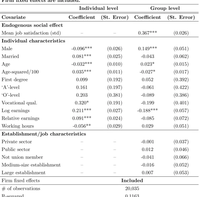
We also report estimates for contextual social effects. At the workplace level,

we find that individual-level job satisfaction goes up with the fraction of male

and older workers in the workplace. At the local labor market level, however,

8

(31)

gender and age do not have any statistically significant contextual effect;

in-stead, we only find that individual-level job satisfaction score goes down as the

fraction of workers with greater access to promotion opportunities goes up in

each industry _× region cell. We also document that there are significant “in-come comparison effects” at the workplace, but not at the local labor market.

In particular, we find that individual-level job satisfaction goes down with (i)

average earnings and (ii) fraction of high earners—i.e., those who earn above

the median wage within the relevant worker population—in the workplace.

We discuss these results further in Section 2.5, where we also present detailed

robustness exercises to prove that our estimates are not excessively sensitive

to relaxing some of the main assumptions behind the empirical model.

The plan of the paper is as follows. Section 2.1 relates and compares our work

to the relevant papers in the literature. Section 2.2 explains the details of

the econometric model and the identification strategy we employ. Section 2.3

provides an overview of the data sets we use and justifies the construction of our

reference groups in different work settings. Section 2.4 presents the estimates,

discusses in detail the results, performs robustness checks, and elaborates on

the policy implications. Section 2.5 concludes.

2.1 Related Literature

Our paper can be placed into the literature investigating social interactions

in labor markets. There is a large body of literature testing the existence of

(32)

absenteeism, and learning (or knowledge spillovers). The results are mixed.

For example, using grocery scanner data from a large supermarket chain,Mas and Moretti (2009) perform a field experiment among low-wage earners to analyze if the individual-level effort is influenced by a permanent increase in

the productivity of co-workers and find reasonably large peer effects. Falk and Ichino (2006) study the behavior of high school students performing a simple task in a laboratory experiment to understand if individual-level performances

are directly affected by the existence of other individuals doing the same task

and they also document moderate peer effects. Ichino and Maggi (2000) find that group-level peer absenteeism increases individual absenteeism. In a field

study, Bandiera et al. (2009) find that individual-level productivity responds to the level of a friend working nearby, but does not respond to the

skill-level of a non-friend working around. Guryan et al. (2009), on the other hand, find employing a random assignment exercise on a golf tournament data

that individual-level performance is not influenced by the playing partners’

ability. Cornelissen et al.(2013) report only small peer effects in wages among co-workers.9

While Azoulay et al. (2010) andJackson and Bruegmann (2009) document significant knowledge spillovers among co-workers,Waldinger(2012) shows that those spillovers are weak, if they ever exist.

There are also several papers investigating contagion effects in subjective

well-being measures. Using Chinese rural survey data, Knight and Gunatilaka (2009) examine whether happiness is infectious or not at the village level. Their results show that happiness is infectious in narrowly-defined reference

9

(33)

groups. They exploit the panel feature of their data set to remove the reflection

problem and identify the relevant social effects. Papers in the psychology

literature also find that happiness might be contagious in small environments.10

However, these studies do not address the reflection problem, which might bias

the results. Tumen and Zeydanli (2014), on the other hand, find that these contagion effects might disappear in more broadly defined reference groups.

Our paper differs from this body of work and contributes to the related

lit-erature in three ways. First, this is the first paper in the litlit-erature

estimat-ing spillover effects in job satisfaction. We show that there exist statistically

and economically significant job satisfaction spillovers in various work

environ-ments. Second, we show that the degree of these spillover externalities may

change at different aggregation levels. Using two different data sets from the

United Kingdom, we construct our reference groups at two aggregation levels:

workplace level and local labor market level. The former defines peer effects in

narrowly defined work settings, while the latter defines the social environment

in larger ecological settings that embed more general aspects of community

and working life. We document that the job satisfaction spillovers exist in

both environments; but, they are much stronger at the workplace level than

local labor market level. We further argue that this may have important

pol-icy implications. And, third, motivated by the hierarchical models of social

processes, we develop an original identification strategy to separate

endoge-nous effects from the contextual effects, controlling for group-level unobserved

heterogeneity.

10

See, e.g.,Hatfield et al. (1994),Sato and Yoshikawa (2007), and Fowler and Christakis

(34)

There are also several papers criticizing the empirical literature on peer

ef-fects.11

In particular, Angrist (2014) has pointed out that many papers in the literature falsely interpret the observed correlations between

individual-and group-level outcomes as causal relationships. He argues that the

instru-mental variable (IV) estimates reported in this literature “often ... produce

findings that look like a peer effect, even in a world where behavioral influences

between peers are absent.” In this paper, we do not use the IV approach;

in-stead, we rely on a non-linear model of social interactions—which is motivated

by hierarchical statistical models—to obtain econometric identification. The

non-linear models are not free of problems, either. The most common criticism

is that, most of the time, the non-linear structure used to identify peer effects

is hard to justify. The non-linear specification that we use in this paper has

two appealing features. First, the non-linearity is simply obtained by including

certain interaction terms between the regressors of a standard linear-in-means

model. The use of interaction terms is quite common in regression analysis and

are never regarded as strange or unjustified. Second, the inclusion of

interac-tion terms into linear-in-means models is theoretically justified by the “social

ecologies” viewpoint in a strand of the sociology literature.12

See Raudenbush and Sampson (1999) and Blume and Durlauf (2005) for further motivation and references. Next, we present the details of our non-linear model of social

interactions and describe our identification strategy.

11

See, e.g.,Moffitt(2001), andAngrist(2014). 12

(35)

2.2 Model and Theoretical Background

The econometric framework that we employ in this paper is a version of the

canonical linear-in-means model of social interactions. Our ultimate goal is

to estimate social interactions in job satisfaction. In particular, we would like

to estimate the effects of (1) group-level job satisfaction—the “endogenous

social effect”—and (2) group-level exogenous characteristics—the “contextual

effects”—on individual-level job satisfaction, controlling for group-level

hetero-geneity. The linear-in-means model of social interactions is plagued with the

well-known “reflection problem,” which masks the econometric identification

of social interactions [Manski(1993)]. The simplest way to resolve this issue is to use an appropriately formulated instrumental variables strategy. When an

instrument is not available, it is necessary to invoke non-linearities to identify

social interactions [Brock and Durlauf (2001a),Blume et al. (2011)].

In this paper, we use an empirical strategy that allows us to convert the

stan-dard linear model into a nonlinear one. The motivation comes from the

hier-archical models of social processes. This hierhier-archical structure secures

iden-tification of social interactions via introducing cross-product terms into the

standard model. This section provides a detailed description of our

economet-ric model for the purpose of familiarizing the reader with the basic concepts

we frequently mention throughout the paper. Section 2.2.1 presents our

em-pirical model and the associated technical issues (i.e., the reflection problem)

including a formal statement of the conditions required to identify social

(36)

how we achieve identification.

2.2.1 The Empirical Model of Social Interactions

Each individual i _{∈ I} is a member of a group g _{∈ G}, where _I is the number of individuals in the worker population and _G is the number of groups, with I >G. The following linear-in-means equation is an empirical tool commonly used in the literature:

ωig =β0+β1X_ig +β2Y_g+Jm_g+u_g+ǫ_ig, (2.1)

where the dependent variable, ωig, is the individual-level job satisfaction for

person iin groupg, Xig is a vector of individual-level observed characteristics

of i in group g, Yg is a vector of group-level observed characteristics of group

g,mg =E[ωig|g, Fig] is the mean job satisfaction in group g,ug is a group-level unobserved factor common across the members of groupg, andǫig is a random

error term with E[ǫig|g, Fig] = 0. In our notation, Fig corresponds to the empirical distribution of individuals in groupg and this distribution is possibly

different for each group. The distinction between β2 (contextual effects) and

J (endogenous effect) is the key notion in this model. The former measures

the effect of exogenous group-level variables on the individual-level outcome,

while the latter measures the effect of endogenous group-level outcome on

the individual-level outcome. Our ultimate goal is to clearly distinguish β2

from J and to separately identify the effects of group-level variables on the

(37)

issue in this standard setting. In what follows, we shut down the group-level

unobserved effect ug for notational simplicity. It will reappear in our final

equation.

To define the identification problem, we take the conditional mathematical

expectations of both sides of the linear-in-means equation, where the

condi-tioning is ong and Fig, for all i and g. This gives us

mg =β0+β1X_g+β2Y_g+Jm_g, (2.2)

where Xg = E[Xig|g, Fig]. Xg can be named as the group-level mean of individual-level observed characteristics and it may or may not coincide with

Yg. Notice that mg appears in both sides of Equation (2.2). Solving for mg yields the result that

mg =

β0

1−J + β1

1−JXg+ β2

1−JYg. (2.3)

The reflection problem states that if the dimensions of the vectors Xg and

Yg are the same, then linearity masks the econometric identification of the

(endogenous) social interactions parameter J.

To formalize this statement, we plug Equation (2.3) into Equation (2.1), which gives us the estimating equation

ωig =

β0

1−J +β1Xig + Jβ1

1−JXg+ β2

(38)

When the reflection problem is in effect, J and β2 cannot be distinguished

from each other, which implies that social interactions cannot be identified.

To see this, set Xg =Yg, which yields the equation

ωig =

β0

1₋J +β1Xig +

Jβ1+β2

1₋J Yg+ǫig. (2.5)

It is obvious that, in this equation, it is impossible to separate J from β2

econometrically. One solution is the existence of an additionalXg which is not

inYg. If such an Xg exists, then endogenous social interactions (J)—and also

all the other model parameters—are identified by applying simple ordinary

least-squares method on Equation (2.4). In other words, one individual-level variable, the mean of which cannot be regarded as a group-level variable, is

required for identification of social interactions.

Unfortunately, most of the large data sets—such as BHPS, GSOEP, WERS,

etc.—do not include a variableXg that can naturally fit into the IV definition

provided above. One popular alternative to IV is to introduce non-linearities

into the linear-in-means specification. To demonstrate how non-linearities

se-cure identification, we modify the standard model as follows:

ωig =β0+β1X_ig +β2Y_g+Jφ(m_g) +ǫ_ig, (2.6)

(39)

rearranging the terms in such a way that the terms with mg appears on the

left and the rest of the variables on the right, we get the equation

Φ(mg) =β0+β1X_g+β2Y_g, (2.7)

where Φ(mg) = mg − Jφ(mg). The functions φ(·) and Φ(·) has the same properties, therefore we can invert Φ(_·) to get

mg = Φ−

1

(β0+β1X_g+β2Y_g) (2.8)

and plugging this into the original estimating equation we get

ωig =β0+β1X_ig +β2Y_g+Jφ

Φ−1

(β0+β1X_g+β2Y_g)

+ǫig. (2.9)

In such a setting, we can identify β2 and J separately without a further need

for an exclusion restriction (or an IV). One problem with this framework is

that there is no systematic way of choosing the functional form ofφ(·). In this paper, we propose an estimation strategy that introduces a systematic way to

embed non-linearities into the standard empirical specification. To be specific,

we construct a hierarchical model, which has the additional advantage of being

consistent with our definition and conceptualization of social interactions in

(40)

2.2.2 The Hierarchical Model

Suppose that the Equation (2.1) is modified as follows:

ωig =α0(Y_g) +α1(Y_g)X_ig +α_J(Y_g)m_g+u_g+ǫ_ig. (2.10)

In words, the coefficients α0, α1, and α_J are stated as functions of the

con-textual variables, Yg, which define the “social context.” In other words, the

contextual variables describe the properties of the environments that the

in-dividuals live in. Setting up the regression coefficients in this way implies

that social groups describe ecologies in which decisions are made and matter

because different ecologies induce different mappings from the individual

de-terminants of these behaviors and choices.13

To convert this setting into an

empirical equation that we can estimate, we make the following simplifying

assumptions:

α0(Y_g) =β0+β2Y_g,

α1(Y_g) =β1+bY_g,

αJ(Yg) =J +πYg.

13

(41)

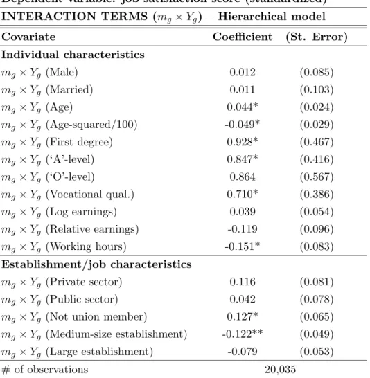
Plugging these expressions into Equation (2.10) yields

ωig =β0+β1Xig +β2Yg+Jmg+πYgmg+Yg′BXig +ug+ǫig, (2.11)

where B is the matrix form of the coefficient vector b. This equation looks

very similar to our original linear-in-means specification except that we include

interaction terms in the form of cross products motivated by the hierarchical

model.

Note that the nature of the unobserved group-level effect ug is a crucial issue.

There are two alternatives: random effects versus fixed effects. If the true

unobserved group-level effect can be controlled for up to a random error term,

then a common way to resolve this issue is to assume thatug is itself random

rather than fixed. Assuming that ug is random is equivalent to saying that it

is uncorrelated with the regressors. However, group-level unobserved factors

can easily be argued to be correlated with, say, group-level job satisfaction.

When this is the case, not being able to control group fixed effects will yield

erroneous results. In our baseline analysis, we assume that ug is a random

term. We then relax this assumption and control for group-level fixed effects

to check if the results differ [see Section 2.4]. We also cluster standard errors

at the group level, which means that we account for within-group correlations

in the error structure.

To demonstrate how this model is identified, we take the conditional

(42)

for mg, which gives us

mg =

β0+β1X_g +β2Y_g+Y_g′BX_g

1−J−πYg

. (2.12)

Notice that, very similar to the motivation behind the nonlinear model, this

model also introduces non-linearity betweenmg and the other regressors, even

when Xg =Yg. There is no need for an exclusion restriction and econometric

identification of social influences is immediate, given standard conditions on

individual- and group-level observed covariates [seeBlume and Durlauf(2005) for further details]. This formulation is consistent with our hypothesis and our

definition of social interactions.

At the end, we estimate Equation (2.11) to separately identify β2 and J. In

this setup, the endogenous social effect is J +πY¯g, where Y¯g are the sample

means of group-level variables, i.e., the endogenous effect is no more J since

we have cross-product terms in the regressions. The same logic applies to the

contextual effects we estimate. The estimates we report and discuss in Section

2.4 directly refer to these “marginal effects.”

2.3 Data and Reference Groups

In this section, we provide a detailed description of the two data sets we use in

our empirical analysis: Workplace Employment Relations Survey and British

Household Panel Survey. Both of these surveys are nationally

(43)

detail the construction of our reference groups for both of these data sets. We

focus on the 2004 editions of both data sets.

2.3.1 Workplace Employment Relations Survey (WERS)

WERS is a national survey of British employees constructed for the purpose

of collecting information on employment relations in Britain.14

The survey

provides information about workers, working conditions, and industrial

rela-tions from all sectors except primary industries and private households with

domestic staff. WERS 2004—the version that we use in our analysis—is the

fifth among a series of surveys. Previous surveys are conducted in 1980, 1984,

1990, and 1998. In the 2004 cross-section, there are around 2,300 workplaces,

1,000 employee representatives, and 22,500 employees.

We construct the job satisfaction scores using the following seven question in

the WERS-2004 data set. How satisfied are you with

1) the sense of achievement you get from work?

2) the scope for using your own initiative?

3) the amount of influence you have over the job?

4) the training you receive?

5) the amount of pay you receive?

6) the job security?

7) the work itself?

14

(44)

The responses are based on a five-point scale with 1 representing “very

satis-fied,” 2 “satissatis-fied,” 3 “neither satisfied nor dissatissatis-fied,” 4 “dissatissatis-fied,” and 5

“very dissatisfied.” For each of the seven questions listed above, we construct

a binary variable for the positive responses—taking the value 1 for the “very

satisfied” or “satisfied” responses and 0 otherwise—and, then, we construct a

sum of the seven binary variables for each individual to form an index with

values from 0 to 7 [see also Jones et al.(2009), Jones and Sloane (2010), and Mumford and Smith (2013)].15

We use this aggregate measure as the “job

satisfaction score” in our analysis. The average job satisfaction score in our

sample is 4.20 and the standard deviation is 2.13. The BHPS data set, which

we describe in the following subsection, has a 1–7 scale constructed based on

different principles. For the sake of comparability of the estimates, we

stan-dardize the main job satisfaction measures in both WERS and BHPS around

zero mean and unit variance. Thus, the dependent variable in our analysis will

be the “standardized job satisfaction.”

We control for a large set of individual- and job-related characteristics. To

achieve consistency between the two data sets, we construct the WERS

vari-ables similar to their counterparts in the BHPS data set. After excluding

miss-ing information on our control variables and droppmiss-ing workplaces with less than

two employees, the WERS data set includes 1,673 workplaces/establishments

and, in each workplace, up to 25 randomly-chosen employees taking the

ques-15

(45)

tionnaire.16

We start with describing the education variables. Since this is

a workplace-level data set, “No Qualification” category includes only a very

small number of observations; thus, we drop the observations in this category

and concentrate on the following education levels: “Higher Degree” (refers

to postgraduate education), “First Degree” (refers to college education),

“A-level,” “O-level” (both referring to different classes of high-school education),

and “Vocational Qualification.”17

Earnings variable in the WERS is reported

in 14 pre-specified intervals,18

and, following Mumford and Smith (2009), we use the midpoints of these intervals as our earnings variable for each individual.

The last interval is open ended, so it does not have a midpoint; instead, we use

the mean earnings for the last interval. In our sample, the average weekly log

earnings is around 5.7. We also include relative earnings as a dummy variable

taking 1 if the employee earns more than the mean earnings in the sample.

We categorize the job status under three sector categories: private sector job,

public sector job, and other. An establishment size variable is generated from

the question of “Currently, how many employees do you have on the payroll at

this establishment?” The answer varies from 5 to 10,000. We construct three

variables for establishment size; small establishment (less than 50 employees),

medium-size establishment (between 50 and 200 employees), and large

estab-lishment (more than 200 employees). Working hours are simply represented

16

For consistency, the individuals in the BHPS data set who work in firms with less than two employees are correspondingly dropped.

17

To be concrete, after constructing our sample, we observed that only two individuals remained in the data with no school degrees. We think that dropping these two observations would be more reasonable than generating a new education category called “no degree.” Such a category, on the other hand, exists in our BHPS sample since the number of individuals with no degree is non-negligible in the BHPS data.

18

(46)

as a dummy variable taking 1 if the actual hours worked is above the sample

mean and 0 otherwise.

Among 20,035 employees and 1,673 establishments in our sample, the average

age is 42, 47 percent are male, and 68 percent are married. Higher degree

has the lowest fraction, whereas vocational qualifications have the highest. 46

percent of the employees are union members. 55 percent of the workplaces

are publicly owned. Regarding the establishment size, the shares of small,

medium, and large establishments are 0.32, 0.32, and 0.36, respectively. See

Table (2.1) for detailed summary statistics for our WERS sample.

2.3.2 British Household Panel Survey (BHPS)

The BHPS provides information on individual-, household-, and

job/employer-related characteristics from 1991 to 2008 in England, Scotland, Wales, and

Northern Ireland. It yearly follows the same representative sample of

house-holds interviewing every adult member of sampled househouse-holds. Eighteen waves

of data are available. To make the two data sets comparable and compatible,

we focus on the 2004 cross-section of the BHPS.

The individual-level job satisfaction in the BHPS data set is reported based

on a seven-point scale ranging from 1 (not satisfied at all) to 7 (completely

satisfied). The employed workers are asked to rate the job satisfaction levels

regarding the total income, job security, the actual work itself, and hours

worked. The last question about job satisfaction is “Overall, how satisfied

(47)

the 1–7 scale and used as the “job satisfaction score” in our analysis. As we

explain above, we standardize the job satisfaction score around zero mean and

unit variance to achieve consistency across the job satisfaction measures we

use for the WERS and BHPS data sets.

For the individual-level observed characteristics, we control for gender, age,

education level, marital status, earnings, and pay comparisons. We collapse

the education-levels into seven broad groups as follows: higher degree refers

to postgraduate education, first degree refers to college education, A-level,

O-level, and other higher qualification refer to high school graduates of different

types (consistent with the education system in the UK), vocational

qualifica-tion refers to teaching, nursing, commercial, apprenticeship, and the certificate

of secondary education (CSE), and, finally, the ones withno qualification. The

earnings variable—usual gross pay per month: current job—is recorded as the

actual amount received and, thus, we simply take the natural logarithm of

this variable in our analysis. We also consider the “taste for working hours”

variable. Promotion opportunities is described by the binary variable taking

1 if the worker has access to promotion opportunities and 0 otherwise. The

rest of the variables—firm size, job status, relative earnings, and union

mem-bership—are constructed similar to their counterparts in our WERS sample.

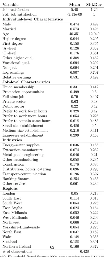
Table (2.2) presents the summary statistics of the sample that we use in our analysis. In order to be included into our sample, the respondent have to be

employed and report a job satisfaction score. The mean age of the respondents

(48)

married, 4.4 percent have higher degree, 15.8 percent have first degree, another

12.6 percent have A-level degree, 17.6 percent have O-level degree, 30.8 percent

have other higher qualifications, 9.4 percent have vocational qualifications, and

the remaining 9.4 percent have no qualifications. Before standardization, the

mean job satisfaction score is approximately 5.4 out of 7, with a standard

deviation of 1.26. 79 percent are employed in full-time jobs. 63 percent are

employed in privately-owned firms. 32.8 percent prefer to work fewer hours.

48.6 percent are employed in small-size firms. See Table (2.2) for further information on region- and industry-specific details. We generate group-level

variables based on our reference groups constructed as industry_×region cells. Below we describe how we construct our reference groups both in the WERS

and BHPS data sets.

2.3.3 Reference Groups

Our primary objective is to separately identify endogenous social effects and

contextual social effects in job satisfaction within a formal empirical model of

social interactions. We conceptualize the social interactions that we estimate as

the existence of “spillovers” in the society in the sense that the group-level job

satisfaction in one’s reference group affects the individual worker’s perception

of own job satisfaction. We perform this task at two levels with two different

data sets from the United Kingdom. First, we use the WERS data set to

estimate spillovers at the workplace level. And, second, we use the BHPS data

set to estimate job satisfaction spillovers at the local labor market level. The

(49)

interacting. The BHPS data set, on the other hand, captures social effects

among individuals who are potentially interacting indirectly. As Bramoulle et al. (2009) clearly state, this type of social effects is based on the idea that “neighbors in the neighborhood do not affect me directly; what matters is the

neighborhood itself.”

WERS_{. The WERS data sets naturally offers establishment-level reference}

groups; that is, all workers employed in a given establishment constitute the

reference group for each of the workers employed in that establishment. There

are 1,673 establishments in our WERS sample. Thus, the number of reference

groups is 1,673. The average group size is approximately 12 worker per

es-tablishment. This setting defines narrow reference groups hypothesizing that

social forces operate at the workplace level: workers in a given establishment

are exposed to similar work-specific conditions that shape their job satisfaction

perceptions. The group-level counterparts of the individual-level variables are

constructed taking averages at the workplace level. Similarly, the endogenous

social variable (the group-level job satisfaction score) is calculated by averaging

the job satisfaction scores within the workplace.

BHPS_{. For the BHPS data set, we construct industry} _× _{region cells as our}

reference groups. In terms of our conceptualization of social interactions, this

means that we try to capture the social forces that operate among workers

who are geographically close to each other and who are potentially exposed

to similar local labor market conditions specific to the industries they belong

(50)

social interactions studies, particularly the ones handling large data sets. For

example, Luttmer (2005) utilizes the outgoing rotation groups feature of the Current Population Survey and constructs industry _× occupation cells to es-timate the neighborhood effects of income on individual-level happiness.

Sim-ilarly, Ferrer-i-Carbonell (2005) uses the German Socio-Economic Panel and constructs education_×age _×region cells to estimate the impact of the group-level income on individual-group-level subjective well-being. In a similar context,

Glaeser et al.(1996) construct region-specific cells on a lattice to estimate the impact of neighbors’ criminal-activity decisions on the agent’s own decision to

participate in crime. In another example, Stutzer and Lalive (2004) use data from Switzerland cantons and construct canton-level cells to estimate the effect

of social norm to work—roughly, the rate of employment in one’s

neighbor-hood—on how quickly the unemployed individual finds a job, probably due to

social pressure. The examples can be extended further. In all of these papers,

large reference groups are constructed to capture the peer influences in broad

social settings.

In our BHPS sample, the following twelve regions describe the geographical

clustering: 1) London, 2) South East, 3) South West, 4) East Anglia, 5) East

Midlands, 6) West Midlands, 7) North West, 8) North East, 9) Yorkshire &

Humberside, 10) Wales, 11) Scotland, and 12) Northern Ireland. Nine industry

categories are selected at one-digit level as follows: 1) energy & water supplies,

2) extraction of minerals & manufacture of metal goods, mineral products &

chemicals, 3) metal goods, engineering & vehicles, 4) other manufacturing

ESSAYS ON SUBJECTIVE WELL-BEING

ESSAYS ON SUBJECTIVE WELL-BEING

A Ph.D. Dissertation

by

TUGBA ZEYDANLI

European Doctorate in Economics Erasmus Mundus (EDE-EM)

Paris School of Economics, Universit`e Paris I:

Panth`eon-Sorbonne

Nova School of Business and Economics, Universidade Nova de

Lisboa

ABSTRACT

ESSAYS ON SUBJECTIVE WELL-BEING

ACKNOWLEDGEMENTS

TABLE OF CONTENTS

LIST OF TABLES

LIST OF FIGURES

CHAPTER 1

INTRODUCTION

1.1

Social Interactions in Job Satisfaction

1.2

Selection Correction on Day-Of-The-Week

1.3

Competitive Elections and Ethnic

Identi-fication

1.4

Thesis Outline

CHAPTER 2

SOCIAL INTERACTION IN JOB

SATISFACTION

2.1

Related Literature

2.2

Model and Theoretical Background

2.2.1

The Empirical Model of Social Interactions

2.2.2

The Hierarchical Model

2.3

Data and Reference Groups

2.3.1

Workplace Employment Relations Survey (WERS)

2.3.2

British Household Panel Survey (BHPS)

2.3.3

Reference Groups