TIME CROSS HOLE TOMOGRAPHY
Armando Luis Imhof,
1Carlos Adolfo Calvo
2Recebido em 16 dez. 2003 / Aceito em 28 maio 2004 Received dec. 16, 2003 / Accepted may 28, 2004
ABSTRACT
It was developed a simple and high speed method with the purpose to model inclusions of irregular forms (simply connected and convex domain) in the context of cross hole travel time 2D tomography. The extension to 3D can be easily implemented and is not covered in this paper.
The following assumptions were made:
a) Homogeneus host medium (therefore straight ray propagation assumed) b) Homogeneus inclusion.
c) Not very high velocity contrast between host medium (V1) and the inclusion (V2).
The algorithm calculate the host velocity V1 considering the (straight) ray between source 1 and receiver 1, and considering that this ray not intersect the anomaly. Then the velocity V2 of the inclusion is estimated upon determining the difference δt among measured times sourcei- receiverj and corresponding calculated times. If the global difference is negative signifies that V2 will be greater than V1 and viceversa. The small values of δt are treated as outliers and therefore eliminated. The last initial parameters needed by the algorithm are the coordinates of the center of the inclusion, which are estimated by a graphical procedure.
Afterwards the program approximates the contour of the inclusion using the Nelder-Mead ‘simplex’ algorithm. At last the perfomance of the algorithm was applied with real data.
Keywords::::: Tomography, Cross Hole, Simplex Downhill, Variational, Nelder Mead.
RESÚMEN
Se desarrolló un método simple y veloz para modelar inclusiones de formas irregulares (dominio convexo, simple conexo) en el contexto del método de tomografía sísmica en cross hole 2D. La implementación a 3D es fácil de llevar a cabo y no es tratada en este trabajo.
Las siguientes premisas se tuvieron en cuenta:
a) Homogeneidad del sustrato (por consiguiente se consideró la teoría de propagación de rayo recto). b) Inclusión homogénea.
c) Un bajo contraste de velocidades entre el sustrato (V1) y la inclusión (V2).
El algoritmo calcula la velocidad del sustrato V1 considerando el rayo (recto) entre la fuente ‘1’ y el receptor ‘1’ (superiores) y considerando que este rayo en particular no intersecta la anomalía. Luego la velocidad V2 de la inclusión se calcula a partir de la diferencia dðt entre los tiempos medidos fuente ‘i’ receptor ‘j’ y los correspondientes tiempos calculados con las premisas citadas. Si la diferencia global es negativa significa que V2 es mayor que V1 y viceversa. Los valores muy pequeños de dðt son tratados como puntos fronterizos y no tenidos en cuenta.
Los últimos parámetros iniciales necesarios por el algoritmo son las coordenadas del centro de la inclusión, las cuales se estiman a partir de un procedimiento gráfico.
Posteriormente el programa aproxima el contorno de la inclusión mediante el empleo del algoritmo ‘simplex’ de Nelder Mead. Por último el funcionamiento del programa se puso a prueba con datos reales.
Palabras Clave: Tomografía, Cross Hole, Simplex Downhill, Variacional, Nelder Mead.
1 Instituto Geofísico Sismológico Volponi / Facultad de Ciencias Exactas Físicas y Naturales. Ignacio de la Roza y Meglioli. Rivadavia. C.P. 5400, San Juan, República Argentina. Fax: (54) 264 4234980. Tel.: 54 264 4945015. E-mail: [email protected].
INTRODUCTION
It was developed a simple and high speed algorithm with the purpose to delineate inclusions in the context of cross hole 2D tomography.
The assumptions made were:
a) Homogeneus host medium (therefore straight ray propagation assumed)
b) Homogeneus inclusion.
c) Not very high velocity contrast between host medium (V1) and the inclusion (V2).
The third assumption due to the fact that the algorithm consider that the acoustic impedance (z=ρ.V) among both media do not differ very much.
In a real case the error due to these assumptions is expected not to be large due to the fact that it was proven that a small perturbation in travel time (say 1%) represents an alteration in travel distance (due to refraction mainly) up to 7% (SANTAMARINA; CESARE, 1994).
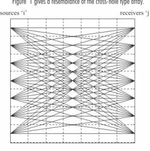
Figure 1 gives a resemblance of the cross-hole type array.
Figure 1 – Crosshole tomographic survey. 7 Sources and 7 receivers array. Raypaths.
Figura 1 – Dispositivo Tomográfico en Cross Hole. Arreglo con 7 fuentes y 7 receptores. Trayectorias de Rayos.
BASIC THEORY
At each reception point (rj) it was calculated the corresponding travel time from source ‘si’ to receiver ‘rj’, conforming the travel time matrixT:
T=
{
tij}
i n j m = = 1 1 ... ...
DenotingDijthe distance from si to rj:
D D
D s r
ij
ij i j
=
{
}
= −
Then the tij are:
t D V ij ij = 1
If there exists an anomaly (medium with velocity V2) insert in medium 1, the matrix of travel times Tis altered and it is formed a new matrix T’:
T’=
{
t’ij}
Inside the inclusion the ij-ray travels a dij distance with velocity V2. Figure 2 represents this situation:
Figure 2 – Raypath inside and outside the inclusion. Figura 2 –Trayectoria de un rayo dentro y en el exterior de la inclusión.
The computation of the travel time is:
t’ij=tij + tij
1 2
∆
wheret’ij is the ij-th perturbed travel time due to the inclusion presence; tij
1
is the travel time in host medium and ∆tij
2
into the anomaly. Writing the equation in terms of velocity and distances:
t D
V d V V
ij ij ij ’ = + . −
1 2 1
1 1
In matrix notation:
T T d V V ’= + . − 1 1 2 1
Note that in real situations T’ corresponds to the matrix of meas-ured travel times.
Extracting the matrix ‘d’ of travel distances into the anomaly gives:
d T T V V V V =( − ) − ’ . 1. 2
It is important to note that the matrix ‘d’ has non zero-ele-ments corresponding to the rays that intersect the inclusion. Later when proccesing these elements dij; there must be annulated those with val-ues near zero (treated as outliers).
It was assumed that the inclusion pertains to a simply connected and convex domain whose contour ‘C’ is a soft curve provided that everyi-j ray intercepts C in two points (except for the tangency points). Any convex domain fulfill this condition.
Let be these intersection points Pij in and
Pij
out (Figure 2)
Then the distances dij will be:
dij Pij P
out ij
in
= −
VARIATIONAL FORMULATION
Lety=y(x) be the contour curve equation . Denoting as ‘L’ to the closed curve length, it appears the functional L = L(y) condi-tioned by matrix ‘d’.
If from the contour Cit is altered ‘y’to ‘y+δy’ (Figure 3) it’ll be seen that ‘L’ turns to be greater; this is equivalent to say that the contour C corresponds to a minimum length solution (always condi-tioned by ‘d’)
Figure 3 – Inclusion contour C and distorted C’. Figura 3 – Contorno de la inclusión C y distorsionado ti.
It was accepted then, as a plausible hipothesis (variational one), that the solution contour correspond to that of minimum length:
solution y / min L(y) (constrained to matrix ‘d’)
Numerical Solution to Variational Calculus
The analitical solution to this variational problem is not possible to obtain in a general case; therefore it was faced by direct methods. These consist to replace the curve y(x) for a finite number of points.
For the inclusion it was replaced the continuous curve for a discretized one with the points Pij
in
and Pij out
, resulting a polygonal with length L* of easy determination.
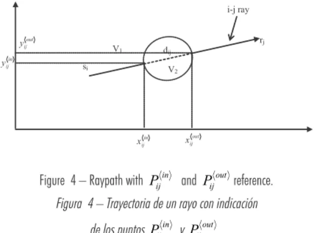
Due to the fact that the matrix of distances ‘d’ is known, Pij out
is easily determined from Pij in
(Xij in
;yij in
) and since ray path of
ij-th ray is known; only Xij in
remains as independent variable (see Figure 4)
Figure 4 – Raypath with Pij in
and Pij out
reference. Figura 4 – Trayectoria de un rayo con indicación
de los puntos Pij in
y Pij out
.
Finally, it stays formulated the problem to get minimum the functionL*:
L*=L*(Xij in
)
where Xij
in is a vector whose ‘p’ components correspond to the rays
that intersects the inclusion.
Computational Implementation
To get minimum the function L*, it was employed the SIMPLEX algorithm of Nelder-Mead (PRESS et al., 1992).
Ann-simplex is a convex polyhedron of ‘n’ dimensions deter-mined by ‘n+1’ vertex (P0,P1,...Pn) linearly independent, whose x points are defined by:
x t Pi i
i n = ⋅ =
∑
0 with0 ≤ t ≤1
i and ti i n = =
∑
1 0SIMPLEX is an algorithm that do not use derivatives; it is slow at the beginning of the iteration process, but nevertheless converges more rapidly in the final stage than other methods (which employ deriva-tives).
Experimental Study
The efficiency of the computational algorithm was demonstrated on real data, which were obtained in the laboratory using sound waves in air. Figure 5 represents schematically the complete installation and the solution parameters.
The objetive was to determine five unknowns with the proposed algorithm:
Vinc,Rinc;Xinc;YincandVback meaning ‘inc’ for inclu-sion and ‘back’ for background.
Figure 5 – Circular Inclusion in homogeneus background. Crosshole array data. Source - Santamarina & Fratta (1998).
Figura 5 – Inclusión Circular en sustrato homogéneo. Arreglo Cross Hole. Fuente - Santamarina & Frata (1998).
As it is represented in Figure 5, the case under study involved a 2D circular inclusion (helium balloon with radius = 23cm) insert in a square image region. Tomographic crosshole data were obtained by ra-diating the host medium (air) from seven discrete source positions (SANTAMARINA; REED, 1994; SANTAMARINA; FRATTA, 1998) and ac-quiring the corresponding records at the receivers on the opposite side. First of all it is necessary to determine which rays intersect the anomaly (from the delay times). Those delay times below a pre-estab-lished margin were discarded with the purpose to discard noise.
Figure 6 represents the rays from the source ‘i’ to the receiver ‘j’that intersects the inclusion. Then it was necessary to evaluate the center coordinates of it by inferential means, clicking with the mouse at the inferred position.
Figure 6 – Rays that intersect the inclusion. Figura 6 – Rayos que intersectan la inclusión.
It is easy to appreciate that the inclusion could be at x = 0.5m. from the origin.
This is the beginning datum. From it the algorithm calculate the
Pijin and Simplex were run calculating the C contour of minimum length. Afterwards the points were interpolated and represented in three forms: a) Representing the raypaths inside the anomaly (Figure 7)
b) Representing the anomaly contour (Figure 8)
Figure 8 – Final contour of the inclusion. Figura 8 – Contorno final de la inclusión.
c) Interpolating the points with an ellipse (Figure 9)
Figure 9 – Final contour of the inclusion (elliptic approximation). Figura 9 – Contorno Final de la Inclusión (aproximada con una elipse)
Solution Parameters (Calculated)
Figure 10 represents a detail of the Xinc,Yincand approxima-tion of Rinc.
The Vback was calculated by the algorithm considering that the raypath among source 1 and receiver 1 (upper) does not intersect the anomaly.
Rinc= 0.26m. Xinc= 0.5m. Yinc= 0.772m. Vinc.= 600m/s Vback.= 349m/s
Figure 10 – Contouring the inclusion with an ellipse. Detail. Figura 10 – Aproximando la inclusión con una elipse. Detalle.
CONCLUSIONS
It was proposed a new and simple method for delimitating ho-mogeneous inclusions into a hoho-mogeneous background which is accu-rate and can model both high and low velocity anomalies.
The method was succesfully applied in more general domains (i.e. simply connected) without the convexity constraint.
The exact circular form is not obtained from the inversion scheme. This is caused by the lack of sources or receivers (or both) in the ‘x’ direction, which diminishes the resolution (SANTAMARINA; REED, 1994; SANTAMARINA; FRATTA, 1998). Inherently, the cross hole configuration is not the optimum to model anomalies accurately. It is necessary to place sources and/or receivers in the ‘x’ direction too.
Because of the straight ray theory assumption was considered, the errors upon the size of the inclusion will be greater when the contrast between host and inclusion velocities increases.
The initial parameters Vback, Xinc and Yinc, needed for an ad-equate start with simplex method were easily calculated with a simple calculus (for Vback) and inferential method (Xinc, Yinc).
Acknowledgements
NOTES ABOUT THE AUTHORS
Armando Luis Imhof
is Geophysicist graduated in Universidad Nacional de San Juan (UNSJ, Argentina) in 1989. Specialist on
Environ-mental Studies from Universidad Nacional de San Luis (Argentina); graduated 2002. Doctoral student at the Engineering Faculty (Universidad
Nacional de Cuyo, Mendoza, Argentina). Researcher at the Instituto Geofísico Sismológico Volponi (Facultad de Cs. Exactas, Fcas y
Naturales - UNSJ) and adjunct professor at the Electrical Prospecting, Geophysics and Astronomy Department (UNSJ) since 1990. Member
of Asociación Argentina de Geofísicos y Geodestas (A.A.G.G.). Topics of main Research: Geophysics applied to mining, geotechnics an
hidrogeological studies.
Carlos Adolfo Calvo
is electromechanical engineer graduated in Universidad Nacional de San Juan (UNSJ, Argentina) in 1978. MSc in
Applied Mathematics and Informatics at Moscow Physics Institute (MEPHI). Main Professor of Mathematics Analysis, Applied Mathematics
and Numerical Methods; Engineering Faculty (U.N.S.J). Researcher on topics covering applied mathematics to solve engineering
prob-lems. Topics of main research: Applied mathematics.
The authors want to thank to professor Juan Carlos Santamarina from Georgia Tech (USA) for permission to use real case data from his laboratory in this paper.
REFERENCES
POTTS, B. D.; SANTAMARINA, J. C. Geotechnical tomography: the effects of diffraction. Geotechnical Testing Journal, [S.l.], v. 16, n. 4, p. 510-517, 1993.
PRESS, W. H. et al. Numerical recipes in Fortran: the art of scientific computing. New York. Cambridge University Press, 1992.
SANTAMARINA, J. C. 2000. Available in: <http://www.ce.gatech.edu/ ~carlos/laboratory/publication/sigma/ch11/ch11.htm
______; CESARE, M. A. Velocity inversion in the near surface: vertical heterogeneity and anisotropy. Internal report. University of Wat+erloo, Canada, 1994.