The 2d Gross-Neveu Model at Finite Temperature and Density with Finite
N
Corrections
Jean-Lo¨ıc Kneur,Laboratoire de Physique Math´ematique et Th´eorique - CNRS - UMR 5825 Universit´e Montpellier II, France
Marcus Benghi Pinto,
Departamento de F´ısica, Universidade Federal de Santa Catarina, 88040-900 Florian ´opolis, SC, Brazil
and Rudnei O. Ramos
Departamento de F´ısica Te´orica, Universidade do Estado do Rio de Janeiro, 20550-013 Rio de Janeiro, RJ, Brazil (Received on 10 September, 2006)
We use the linearδexpansion, or optimized perturbation theory, to evaluate the effective potential for the two dimensional Gross-Neveu model at finite temperature and density obtaining analytical equations for the critical temperature, chemical potential and fermionic mass which include finiteN corrections. Our results seem to improve over the traditional large-Npredictions.
Keywords: Non perturbative methods; Gross-Neveu model; Finite temperature; Finite density
I. INTRODUCTION
The development of reliable analytical non-perturbative techniques to treat problems related to phase transitions in quantum chromodynamics (QCD) represents an important do-main of research within quantum field theories. The appear-ance of large infrared divergences, happening for example in massless field theories, like in QCD [1], close to critical tem-peratures (in field theories displaying a second order phase transition or a weakly first order transition [2]) can only be dealt with in a non-perturbative fashion. Among the analytical non-perturbative techniques one of the most used is the 1/N approximation [3]. Though a powerful resummation method, this approximation can quickly become cumbersome after the resummation of the first leading contributions, like for the N=3 case which regards QCD. This is due to technical dif-ficulties such as the formal resummation of infinite subsets of Feynman graphs and their subsequent renormalization. In this work we employ an alternative non-perturbative method known as the linearδexpansion (LDE) [4] to investigate the breaking and restoration of chiral symmetry within the two dimensional Gross-Neveu model [5] at finite temperature (T) and chemical potential (µ). As we shall see, the LDE great advantage is that the actual selection and evaluation,including renormalization, of the relevant contributions are carried out in a completely perturbative way. Non-perturbative results are generated through the use of a variational optimization pro-cedure known as the principle of minimal sensitivity (PMS) [6]. The two dimensional Gross-Neveu model offers a per-fect testing ground for the LDE-PMS because, apart from sharing common features with QCD, it is exactly solvable in the large-Nlimit. The large-Nresult for the critical tempera-ture (at zero chemical potential) of the Gross-Neveu model is Tc≃0.567mF(0)wheremF(0)is the fermionic mass atT=0. However, due to the appearance of kink–anti-kink configura-tions, the exact critical temperature for this model should be zero [7]. Because kink configurations are unsuppressed the system is segmented into regions of alternating signs of the order parameter, at low temperatures. Then, the net average value of the order parameter is zero. At leading order, the
1/Napproximation misses this effect because the energy per kink goes to infinity asN→∞while the contribution from the kinks has the form e−N. Our strategy will be twofold. First, we show that the LDE-PMS exactly reproduces, within theN→∞limit, the “exact” large-Nresult. Next we show ex-plicitely that already at the first non trivial order the LDE takes into account finiteNcorrections which induce a lowering of Tcas predicted by Landau’s theorem. Here, the calculations are performed for three cases which are: (a)T =0 andµ=0, (b)T 6=0 andµ=0 and (c)T =0 andµ6=0. Our main results include analytical relations for the fermionic mass atT =0 andµ=0,Tc (atµ=0) andµc(atT =0) which include fi-niteNcorrections. The caseT 6=0 andµ6=0, which allows for the determination of the tricritical points and phase dia-gram is more complex, due to the numerics. This situation is currently being treated by the present authors [8]. In the next section we review the Gross-Neveu effective potential at finite temperature and chemical potential in the large-N approxima-tion. The LDE evaluations are presented in section III. The results are discussed in section IV while section V contains our conclusions.
II. THE GROSS-NEVEU EFFECTIVE POTENTIAL AT FINITE TEMPERATURE AND CHEMICAL POTENTIAL IN
THE LARGE-NAPPROXIMATION
The Gross-Neveu model is described by the Lagrangian density for a fermion fieldψk(k=1, . . . ,N) given by [5]
L
= N∑
k=1· ¯
ψk(i6∂)ψk+mFψ¯kψk+ g2
2 (ψ¯kψk)
2
¸
. (1) WhenmF=0 the theory is invariant under the discrete trans-formation
ψ→γ5ψ, (2)
For the studies of the Gross-Neveu model in the large-N limit it is convenient to define the four-fermion interaction as g2N=λ. Sinceg2vanishes like 1/N, we then study the
the-ory in the large-Nlimit with fixedλ[5]. As usual, it is useful to rewrite Eq. (1) expressing it in terms of an auxiliary (com-posite) fieldσ, so that [9]
L
=ψ¯k(i6∂)ψk−σψ¯kψk− σ2N2λ . (3)
As it is well known, using the 1/Napproximation, the large-N expression for the effective potential is [5, 9]
VeffN(σc) =Nσ 2
c 2λ+iN
Z d2p (2π)2ln
¡ p2−σ2
c ¢
. (4)
The above equation can be extended at finite temperature and chemical potential applying the usual associations and re-placements. E.g., momentum integrals of functions f(p0,p) are replaced by
Z d2p
(2π)2f(p0,p)→iT
∑
n Z d p
(2π) f[i(ωn−iµ),p],
whereωn= (2n+1)πT,n=0,±1,±2, . . ., are the Matsubara frequencies for fermions [10]. For the divergent, zero temper-ature contributions, we choose dimensional regularization in arbitrary dimensions 2ω=1−εand carry the renormalization in the MS scheme, in which case the momentum integrals are written as
Z d p
(2π)→
Z
p=
µeγEM2
4π
¶ε/2Z d2ωp
(2π)2ω,
whereM is an arbitrary mass scale and γE ≃0.5772 is the Euler-Mascheroni constant. The integrals are then evaluated by using standard methods.
In this case, Eq. (4) can be written as VeffN(σc)
N =
σ2
c 2λ−T
∑
nZ d p (2π) ln
£
(ωn−iµ)2+ω2
p(σc) ¤
, (5) whereω2
p(σc) =p2+σ2c. The sum over the Matsubara’s fre-quencies in Eq. (5) is also standard [10] and gives for the effective potential, in the large-Napproximation, the result
VeffN(σc)
N =
σ2
c 2λ−
Z
p ωp(σc)
+ T
Z
pln(1+exp{−[ωp(σc) + µ]/T})
+ T
Z
pln(1+exp{−
[ωp(σc)−µ]/T}). (6) After integrating and renormalizing the above equation one obtains
VeffN(σc)
N =
σ2
c 2λ−
1 2π
½ σ2
c ·
1 2+ln
µM
σc ¶¸
+2T2I1(a,b)
¾
,
(7)
where I1(a,b) =
Z ∞
0 dx
· ln
µ 1+e−
√
x2+a2−b
+ (b→ −b) ¸
, (8)
witha=σc/Tandb=µ/T. Taking theT=0 andµ=0 limit one may look for the effective potential minimum ( ¯σc) which, when different from zero signals dynamical chiral symmetry breaking (CSB). This minimization produces [5, 9]
mF(0) =σc¯ =Mexp ³
−πλ´. (9)
10
20
30
Μ 10
20 T
0 0.1
0.2 0.3
mF
10
20
30
Μ
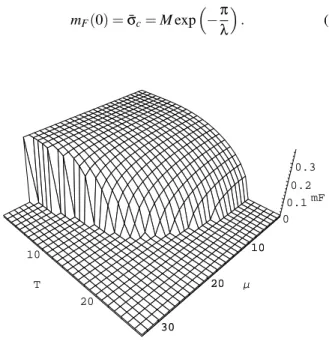
FIG. 1: A three dimensional graph showing the fermionic mass,mF,
as a function ofT andµ. One sees a second order phase transition at µ=0 while a first order transition occurs atT=0. All quantities are in units of 10×Mwhileλ=π.
5 10 15 20 25 30
Μ 5
10 15 20 25
T
5 10 15 20 25 30
Μ 5
10 15 20 25
T
FIG. 2: Top views of figure 1. On the LHS we have a shaded fig-ure where the black region represents CSR. The contour lines of the figure on the RHS indicate an abrupt (first order transition) for small values ofT. Both figures display a (tricritical) point where the smooth descent meets the abrupt one. All quantities are in units of 10×Mwhileλ=π.
the exact value for the critical temperature (Tc) at which chiral symmetry restoration (CSR) occurs can be evaluated analyti-cally producing [11]
Tc=mF(0) eγE
π ≃0.567mF(0), (10) while, according to Landau’s theorem, the exact result should beTc=0. By looking at Figure 1 one notices an abrupt (first order) transition whenT =0. The analytical value at which this transition occurs has also been evaluated, in the large-N limit, yielding [12]
µc= mF(0)
√
2 . (11)
In theT−µplane there is a (tricritical) point where the lines describing the first and second order transition meet. This can be seen more clearly by analyzing the top views of figure 1. Figure 2 shows these top views in a way which uses shades (LHS figure) and contour lines (RHS figure). The tricritical point (Ptc) values can be numerically determined producing Ptc= (Ttc,µtc) = [0.318mF(0),0.608mF(0)][13].
III. THE LINEARδEXPANSION AND FINITEN CORRECTIONS TO THE EFFECTIVE POTENTIAL
According to the usual LDE interpolation prescription [4] the deformed original four fermion theory displaying CS reads
L
δ= N∑
k=1· ¯
ψk(i6∂)ψk+η(1−δ)ψkψk¯ +δ λ
2N(ψkψk)¯ 2
¸
.
(12) So, that atδ=0 we have a theory of free fermions. Now, the introduction of an auxiliary scalar fieldσcan be achieved by adding the quadratic term,
−δ2λN
µ σ+λ
Nψkψk¯
¶2
, (13)
to
L
δ(ψ,ψ). This leads to the interpolated model¯L
δ= N∑
k=1· ¯
ψk(i6∂)ψk−δη∗ψkψk¯ −δ2λNσ2+
L
ct,δ
¸
, (14)
whereη∗=η−(η−σc)δ. The counterterm Lagrangian den-sity,
L
ct,δ, has the same polynomial form as in the original theory while the coefficients are allowed to beδandη depen-dent. Details about renormalization within the LDE can be found in Ref. [14].From the Lagrangian density in the interpolated form, Eq. (14), we can immediately read the corresponding new Feyn-man rules in Minkowski space. Each Yukawa vertex carries a factor−iδwhile the (free)σpropagator is now−iλ/(Nδ). The LDE dressed fermion propagator is
SF(p) = i
6p−η∗+iε, (15) whereη∗=η−(η−σc)δ.
FIG. 3: LDE Feynman graphs contributing up to order-δ. The black dot represents aδηinsertion. The external dashed line representsσc
while the internal line is theσpropagator. The last diagram brings the first finiteNcorrection to the effective potential.
Finally, by summing up the contributions shown in figure 3 one obtains the complete LDE expression to order-δ
Veff,δ1
N (η) = δ
σ2
c 2λ−
1 2π
½ η2
· 1 2+ln
µ M
η ¶¸
+2T2I1(a,b)
¾
+ δη(η−σc) π
· ln
µ M
η 
−I2(a,b)
¸
+ δλη
2
4π2N
( ·
ln
µM
η 
−I2(a,b)
¸2
+J22(a,b) )
.
(16)
whereI1(a,b)is defined by Eq. (8), witha=η/T. Also,
I2(a,b) = Z ∞
0 dx
√
x2+a2
à 1 e√x2+a2+b
+1
+ (b→ −b) !
,
(17) and
J2(a,b) =
sinh(b) a
Z ∞
0
dx 1
cosh(√x2+a2) +cosh(b). (18)
Notice once more, from Eq. (16), that our first order already takes into account finiteNcorrections. Now, one must fix the two non original parameters, δ andη, which appear in Eq. (16). Recalling that atδ=1 one retrieves the original Gross-Neveu Lagrangian allows us to choose the unity as the value for the dummy parameterδ. The infra red regulatorηcan be fixed by demandingVeff,δ1to be evaluated at the point where it is less sensitive to variations with respect toη. This criterion, known as Principle of the Minimal Sensitivity (PMS) [6] can be written as
dVeff,δ1 dη
¯ ¯
¯η¯,δ=1=0. (19)
IV. OPTIMIZED RESULTS
From the PMS procedure we then obtain from Eq. (16), at η=η, the general result¯
½·
Y
(η,T,µ) +η ddη
Y
(η,T,µ) ¸ ·η−σc+η λ
2πN
Y
(η,T,µ) ¸+λT
2
2πNJ2(η/T,µ/T) d
dηJ2(η/T,µ/T)
¾¯
¯
¯η=η¯ =0, (20)
where we have defined the function
Y
(η,T,µ) =lnµM
η 
−I2(η/T,µ/T). (21)
Let us first consider the caseN→∞. Then, Eq. (20) gives two solutions where the first one is ¯η=σcwhich, when plugged in Eq. (16), exactly reproduces the large-Neffective potential, Eq. (7). This result was shown to rigorously hold at any order inδprovided that one stays within the large-Nlimit [15]. The other possible solution, which depends only upon the scales M,T andµ, is considered unphysical [15].
A. The caseT =0andµ=0
Taking Eq. (20) atT =µ=0 one gets
· ln
µM
¯ η
−1 ¸ ·
¯
η−σc−η¯ λ 2πNln
µη¯
M ¶¸
=0. (22)
As discussed previously, the first factor leads to the model independent result, ¯η=M/e, which we shall neglect. At the same time the second factor in (22) leads to a self-consistent gap equation for ¯η, given by
¯
ηδ1(σc) =σc ·
1−2πλNln µη¯
δ1 M
¶¸−1
. (23)
The solution for ¯ηδ1obtained from Eq. (23) is
¯
ηδ1(σc) =Mexp
½2πN
λ +W ·
−2πλNσcM exp µ
−2πλN
¶¸¾
,
(24) where W(x) is the Lambert W function, which satisfies W(x)exp[W(x)] =x.
To analyze CS breaking we then replaceηby Eq. (24) in Eq. (16), which is taken atT =0 andµ=0. As usual, CS breaking appears when the effective potential displays minima at some particular value ¯σc6=0. Then, one has to solve
Veff,δ1(σc,η=η¯δ1) dσc
¯ ¯ ¯δ=
1,σc=σ¯c
=0. (25)
SincemF=σc, after some algebraic manipulation of Eq. (25)¯ and using the properties of theW(x)function, one finds
mF(T =0,µ=0) =M
F
(λ,N) µ1− 1
2N
¶−1
, (26)
where we have defined the quantity
F
(λ,N)asF
(λ,N) =exp ½−λ[1 π −1/(2N)]
¾
. (27)
Eq. (26) is our result for the fermionic mass at first order in
Π 2Π 3Π
Λ
0.20.4 0.6 0.8 1
Σ
c
1
3 10
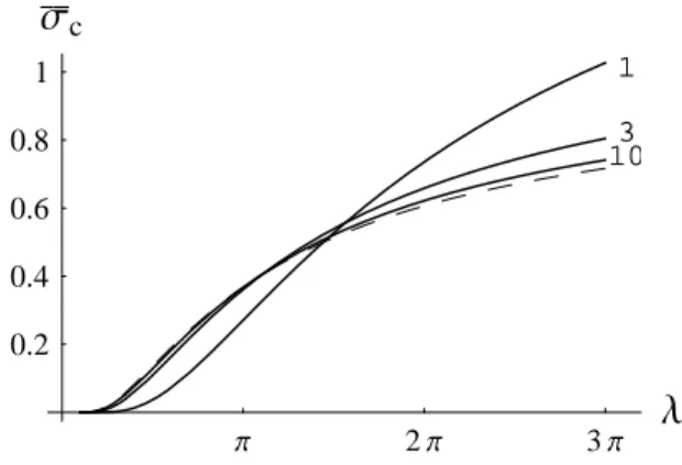
FIG. 4: The effective potential minimum, ¯σc, which corresponds to
the fermionic mass, as a function ofλ forN=1,3 and 10. The dashed line represents the large-Nresult. ¯σcis given in units ofM.
δwhich goes beyond the large-Nresult, Eq. (9). Note that in theN→∞limit,
F
(λ,N→∞) =exp(−π/λ). Therefore, Eq. (26) correctly reproduces, within the LDE non perturbative resummation, the large-Nresult, as already discussed. In Fig. 4 we compare the order-δ LDE-PMS results for ¯σcwith the one provided by the large-N approximation. One can now obtain an analytical result for ¯η evaluated at ¯σc=σc. Eqs. (24) and (26) yield¯
Π 2Π 3Π
Λ
0.2 0.4 0.6
Η
3 10
1
FIG. 5: The LDE optimum mass ( ¯η), evaluated atσc=σ¯c, as a
func-tion ofλforN=1,3 and 10. The continuous lines were obtained from the analytical result, Eq. (28), while the dots represent the re-sults of numerical optimization. ¯ηis given in units ofM.
B. The caseT6=0andµ=0
Let us now investigate the caseT 6=0 andµ=0. In prin-ciple, this could be done numerically by a direct application of the PMS the LDE effective potential, Eq. (16). However, as we shall see, neat analytical results can be obtained if one uses the high temperature expansion by takingη/T =a≪1 andµ/T=b≪1. The validity of such action could be ques-tioned, at first, sinceηis arbitrary. However, we have cross checked the PMS results obtained analytically using the high Texpansion with the ones obtained numerically without using this approximation. This cross check shows a good agreement between both results. Expanding Eq. (8) in powers ofaand b, the result is finite and given by [16]
I1(a≪1,b≪1) =
π2
6 + b2
2 − a2
2 ln
³π
a ´
−a
2
4(1−2γE)
− 7ζ(3)8π2 a2 µ
b2+a
2
4 
+
O
(a2b4,a4b2),(29) and
I2(a,b) =ln
³π
a ´
−γE+7ξ(3) 4π2
µ b2+a
2
2 
+
O
(a4,b4),(30) whereζ(3)≃1.202. If we then expand Eq. (16) at high tem-peratures, up to orderη2/T2, we obtain
Veff,δ1
N = δ
σ2
c 2λ−T
2π
6− η2
2π ·
ln µ
MeγE Tπ
−4(2π)7ζ(3)2
η2 T2
¸
+ δη(η−σc) π
· ln
µ MeγE
Tπ 
−2(2π)7ζ(3)2
η2 T2
¸
+ δλη
2
(2π)2N
· ln2
µMeγE
Tπ 
−7ζ(3)(2π)2ln
µMeγE
Tπ
¶η2
T2
¸
.
(31)
Now, one setsδ=1 and applies the PMS to Eq. (31) to obtain the optimum LDE mass
¯
η(σc,T) = σc ½
1+ λ N(2π)
· ln
µMeγE
Tπ 
− 2(2π)7ζ(3)2
σ2
c T2
· 1+ λ
N(2π)ln µ
MeγE Tπ
¶¸−2#)−1
.
(32) The above result is plugged back into Eq. (31) which, for consistency, should be re expanded to the orderη2/T2. This
generates a nice analytical result for the thermal fermionic mass
¯
σc(T) = ± T
N2p
14πζ(3)λ ·
2Nπ+ln µ
MeγE Tπ
¶¸3/2
×
·
−2Nπ+ (2N−1)λln
µMeγE
Tπ ¶¸1/2
. (33) Figure 6 shows ¯σc(T)/Mgiven by Eq. (33) as a function of T/M, again showing a continuous (second order) phase tran-sition for CS breaking/restoration. The numerical results
illus-0.15 0.17 0.19 0.21
T
0.050.1 0.15 0.2 0.25
Σ
c
FIG. 6: The effective potential minimum, ¯σc, as a function of the
temperature. Both quantities are in units ofMand have been plotted forN=3 andλ=π. The dotted line corresponds to the large result predictingTc=0.208Mwhile the continuous line, which represents
the LDE result, predictsTc=0.170M. In both cases the transition is
of the second kind.
trated by Fig. 6 show that the transition is of the second kind and an analytical equation for the critical temperature can be obtained by requiring that the minima vanish atTc. From Eq. (33) one sees that ¯σc(T =Tc) =0 can lead to two possible solutions forTc.
The one coming from ·
2Nπ+ln
µMeγE
Tcπ ¶¸
=0, (34)
Π 2Π 3Π
Λ
0.10.2 0.3 0.4
T
c1 3 10
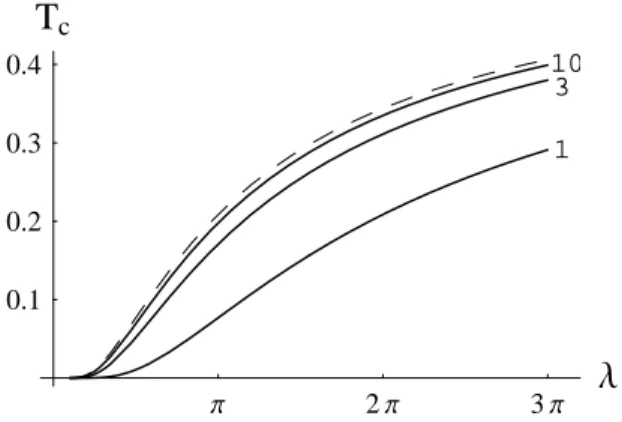
FIG. 7: The critical temperature (Tc), in units ofM, as a function ofλ
forN=1,3 and 10. The continuous lines represent the LDE results while the dotted line represents the large-Nresult.
·
−2Nπ+ (2N−1)λln
µMeγE
πTc ¶¸
=0, (35)
gives for the critical temperature, evaluated at first order inδ, the result
Tc=M eγE
π exp ½
−λ[1 π −1/(2N)]
¾
=Me
γE
π
F
(λ,N) , (36) withF
λ(N)as given before, by Eq. (27). Therefore, Eq. (36) also exactly reproduces the large-N result for N→∞. The results given by this equation are plotted in Fig. 7 in terms of λfor different values of N. The (non-perturbative) LDE results show thatTcis always smaller (for the realistic finiteNcase) than the value predicted by the large-Napproximation. According to Landau’s theorem for phase transitions in one space dimensions, our LDE results, including the first 1/N correction, seem to converge to the right direction.
C. The caseT=0andµ6=0
One can now study the caseT=0,µ6=0 by taking the limit T→0 in the integralsI1,I2andJ2which appear in the LDE
effective potential, Eq. (16). In this limit, both functions are given by
lim T→0T
2I
1(a,b) =−
1
2θ(µ−η) "
η2ln Ã
µ+pµ2−η2
η
!
− µpµ2−η2i, (37)
lim
T→0I2(a,b) =θ(µ−η)ln
Ã
µ+pµ2−η2
η !
, (38)
lim
T→0T J2(a,b) =sgn(µ)θ(µ−η)
p
µ2−η2. (39)
Then, one has to analyze two situations. In the first,η>µ, the optimized ¯ηis given by
½· ln
µM
η 
−1 ¸ ·
η−σc+ λη 2πNln
µM
η ¶¸
− λµ
2
2πN 1 ηln
µM
η
¶¾¯
¯
¯η=η¯ =0, (40)
while for the second,η<µ, ¯ηis found from the solution of
("
η−σc−2πληNln Ã
µ+pµ2−η2 M
!# "
−ln Ã
µ+pµ2−η2 M
!
− η
2
(η2−µ2−µp µ2−η2)
#
−2πληN
) ¯ ¯
¯η=η¯=0. (41)
Note that the results given by Eqs. (37-39) vanish forµ<η. Fig. 8 showsµc, obtained numerically, as a function ofλfor different values ofN. Our result is contrasted with the ones furnished by the 1/N approximation. The analytical expres-sions for ¯ηδ1(σc), Eq. (28), and¯ Tc, Eq. (36), suggest that an approximate solution forµcat first order inδis given by
µc(T =0)≃√M
2
F
(λ,N). (42) It is interesting to note that both results, forTc, Eq. (7), and µc, Eq. (42), follow exactly the same trend as the correspond-ing results obtained from the large-N expansion, Eqs. (10)and (11), respectively, which have a common scale given by the zero temperature and density fermion massmF(0). Here, the common scale is given by ¯η evaluated at σc =σc¯ and T=µ=0, ¯ηδ1(σ¯c) =M
F
(λ,N).V. CONCLUSIONS
Π 2
Π 3Π 2
2Π
Λ
0.10.2 0.3 0.4
Μ
cFIG. 8: The critical chemical potentialµcin units ofM, plotted as
a function ofλforN=3 andT =0. The dashed line represents the 1/N result at leading order, the dot-dashed line represents the 1/Nresult at next to leading order and the continuous line is the first order LDE result.
Tc andµc. However, as far as Tc is concerned the large-N predictsTc≃0.567mF(0)while Landau’s theorem for phase transitions in one space dimensions predicts Tc =0.
Hav-ing this in mind we have considered the first finiteN correc-tion to the LDE effective potential. The whole calculacorrec-tion was performed with the easiness allowed by perturbation the-ory. Then, the effective potential was optimized in order to produce the desired non-perturbative results. This procedure has generated analytical relations for the relevant quantities (fermionic mass,Tcandµc) which explicitely display finiteN corrections. The relation forTc, for instance, predicts smaller values than the ones predicted by the large-Napproximation which hints on the good convergence properties of the LDE in this case. The LDE convergence properties in critical temper-atures has received support by recent investigations concerned with the evaluation of the critical temperature for weakly in-teracting homogeneous Bose gases [17]. In order to produce the complete phase diagram, including the tricritical points, we are currently investigating the caseT6=0 andµ6=0 [8].
Acknowledgments
M.B.P. and R.O.R. are partially supported by CNPq. R.O.R. acknowledges partial support from FAPERJ and M.B.P. thanks the organizers of IRQCD06 for the invitation.
[1] D. J. Gross, R. D. Pisarski, and L. G. Yaffe, Rev. Mod. Phys. 53, 43 (1981).
[2] M. Gleiser and R. O. Ramos, Phys. Lett. B300, 271 (1993); J. R. Espinosa, M. Quir´os and F. Zwirner, Phys. Lett. B291, 115 (1992).
[3] M. Moshe and J. Zinn-Justin, Phys. Rept.385, 69 (2003). [4] A. Okopinska, Phys. Rev. D35, 1835 (1987); A. Duncan and
M. Moshe, Phys. Lett. B215, 352 (1988).
[5] D. Gross and A. Neveu, Phys. Rev. D10, 3235 (1974). [6] P. M. Stevenson, Phys. Rev. D23, 2961 (1981); Nucl. Phys. B
203, 472 (1982).
[7] L.D. Landau and E.M. Lifshtiz,Statistical Physics(Pergamon, N.Y., 1958) p. 482; R.F. Dashen, S.-K. Ma and R. Rajaraman, Phys. Rev.D11, 1499 (1974); S.H. Park, B. Rosenstein and B. Warr, Phys. Rept.205, 59 (1991).
[8] J.-L. Kneur, M.B. Pinto, and R.O. Ramos, in progress. [9] S. Coleman,Aspects of Symmetry(Cambridge University Press,
Cambridge, 1985).
[10] J. I. Kapusta, Finite-Temperature Field Theory (Cambridge University Press, Cambridge, England, 1985).
[11] L. Jacobs, Phys. Rev D10, 3976 (1974); B.J. Harrington and A. Yildz, Phys. Rev. D11, 779 (1974).
[12] U. Wolff, Phys. Lett. B157, 303 (1985); T.F. Treml, Phys. Rev. D39, 679 (1989).
[13] A. Barducci, R. Casalbuoni, M. Modugno, and G. Pettini, Phys. Rev. D51, 3042 (1995).
[14] M. B. Pinto and R. O. Ramos, Phys. Rev. D60, 105005 (1999); ibid.D61, 125016 (2000); J.-L. Kneur and D. Reynaud, JHEP 301,14 (2003).
[15] S.K. Gandhi, H.F. Jones, and M.B. Pinto, Nucl. Phys. B359, 429 (1991).
[16] B. R. Zhou, Phys. Rev. D57, 3171 (1998); Comm. Theor. Phys. 32, 425 (1999).