Mortality tables for the Brazilian
insured population
*Mário Moreira Carvalho de Oliveira**
Milton Ramos Ramirez***
Ricardo Milton Frischtak****
Rafael Brandão de Rezende Borges*****
Bruno Costa******
Ricardo Cunha Pedroso*******
This paper describes the construction of the BR-EMS 2015 mortality tables for the Brazilian insured population. The tables were based on data collected from insurance companies which represent about 80 per cent of the Brazilian insurance market, and they are updates of their previous versions, BR-EMS 2010, which have been the irst mortality tables built with Brazilian market experience. Additional data from government sources was used to improve the information of the companies’ databases. The mortality rates of the population under risk products (death coverage) are remarkably diferent than those under savings products (survivorship coverage); as such, four diferent mortality tables are constructed, separating the population by sex as well as the type of insurance coverage. A straight comparison between the BR-EMS 2015 tables with the statistics of the general Brazilian population shows a striking diference on life expectancies. The BR-EMS 2015 tables are also compared with other life tables.
Keywords: Life tables. Mortality. Death rate. Insurance market. Heligman-Pollard.
* This research received support from Federação Nacional de Previdência Privada e Vida (FenaPrevi); and Fundação de Amparo à Pesquisa do Estado do Rio de Janeiro (Faperj).
Introduction
Over the past few decades, the Brazilian insurance market has expanded at an accelerated rate. Insurance companies operating in Brazil had to resort to foreign and outdated mortality tables in their actuarial analysis and computations, such as the American Annuity 2000 Mortality Table, AT-2000 (JOHANSEN, 1995), since there were no local life tables available based on the Brazilian insurance market.
Following several joint initiatives from the Brazilian government and insurance
companies, the Brazilian association of insurance and pension companies, FenaPrevi,1
through an agreement with the LabMA/UFRJ2 research group, commissioned the
construction of mortality tables for the Brazilian insurance market. The Brazilian regulatory
agency for the insurance market, SUSEP,3 determined the irst version of these tables,
named BR-EMS 2010 (for “Experiência do Mercado Segurador Brasileiro” — Experience of
the Brazilian insurance market), as the as the new oicial standard tables for the Brazilian insurance market. BR-EMS 2010 tables are separated by sex and type of insurance coverage: survivorship (pertaining to old-age pensions) and death (risk products), since the death rates for these two insured groups were shown to be clearly distinct. These tables were built using data from 13 insurance company groups (amounting to about 80 per cent of the Brazilian insurance market) from 2004 to 2006, comprising more than 39 million individuals. The process of building these tables was detailed in the book (DE OLIVEIRA et al., 2012b), which also has an English version (DE OLIVEIRA et al., 2012a).
In 2015, BR-EMS tables were reviewed in order to stay up-to-date with the most current mortality information available at the time. The new version, named BR-EMS 2015, is the current standard for the Brazilian insurance market, published in (SUPERINTENDÊNCIA DE SEGUROS PRIVADOS, 2015). In this revision, data from 2007 to 2012 was incorporated, comprising more than 83 million individuals.
The goal of this paper is to describe and analyse the methodology employed in the construction of Brazilian insurance market tables and perform a comparison with well-established native and foreign mortality tables. Due to the large amount of collected data, parametric models were not used for the entire age range. Instead, we applied a sequence of moving averages to the intermediate age interval in order to smooth the crude rates. We also applied logit patching and exponential itting to smooth the connection of the extreme age intervals to the middle one.
BR-EMS 2015 tables were compared with mortality tables issued by the Brazilian Institute of Geography and Statistics, IBGE,4 for the general Brazilian population. The results
1 In Portuguese, Federação Nacional de Previdência Privada e Vida.
2 The Applied Mathematics Laboratory of the Rio de Janeiro Federal University. In Portuguese, Laboratório de Matemática Aplicada da Universidade Federal do Rio de Janeiro.
show a striking diference between both groups of tables, which reflects the improved socioeconomic conditions of the Brazilian insured population. We also compared other life tables , such as the aforementioned AT-2000, the Chilean table for the insured market, and RV-2009 (SUPERINTENDENCIA DE PENSIONES, 2010), as well as other foreign tables.
The present paper is organized as follows: in section 2, the insurance companies’ databases and efects of their aggregation with government databases are described in more detail, along with some demographic features of the studied population. Section 3 details procedures used to build the curve of death probabilities from crude rates obtained from data. Section 4 contains BR-EMS 2015 tables compared with their previous version, BR-EMS 2010, and with diferent tables from around the world. Final considerations are shown in section 5.
The database
This section describes the whole series of annual data collected from 2004 to 2012 from the 13 insurance company groups participating in the Brazilian mortality tables study commissioned by FenaPrevi. All of this private data was provided to LabMA/UFRJ under a conidentiality agreement with FenaPrevi and the company groups involved.
BR-EMS 2010 tables used data from the three-year period ranging from 2004 to 2006, while BR-EMS 2015 used data from the period from 2004 to 2012. It is worth noting that more than 1.5 billion lines of information have been processed, from around 83 million
individuals. Despite being a unique identiier, the CPF5 (the Brazilian individual taxpayer
registry identiication) cannot be mapped as a key for individuals in the database, since the same CPF code is sometimes used for individuals from the same family in the companies’ databases, or even within the same group of clients of an insurance agent. Thus, in this study, insured individuals were modelled using their attributes of birth date, sex, and CPF, with the extra precaution of allowing only a limited number of individuals with the same CPF code.
During data processing, it was also necessary to deal with undercounting and imprecision of death records of the companies’ databases. For instance, sometimes the death of an individual is not reported by the insurance company, or the death event is misreported as the end of his/her contract (and vice versa). Such data inconsistencies required all informed data records to be checked against the oicial Brazilian social information databases, Cadastro Nacional de Informações Sociais (CNIS) and Sistema Nacional de Óbitos (SISOBI), which have, respectively, information for all pension payments made by the Brazilian Social Security Institute and all deaths registered at all government notary oices in the country. Data from CNIS and SISOBI were obtained through a cooperation agreement with their
legal holder, the Brazilian Ministry of Social Security (Ministério da Previdência Social).
Graph 1 shows annual counts of exposed individuals and deaths, and Graph 2 shows crude mortality rate for each calendar year, which remained stable around 0.26 per cent throughout the years. One can notice a steady growth in the number of exposed individuals, reflecting recent expansion of the Brazilian insurance market along the period. The fluctuations observed in Graph 1 reflect a loss of information due to speciic insurance companies’ database problems in particular years. Graph 1 also shows that the correction provided by the government databases equals 34 per cent of the amount reported by the companies. This represents a fundamental improvement for the computation of the mortality tables.
GRAPH 1
Insured population (before/ater data iltering) and number of death records (before/ater correction with CNIS/SISOBI data)
Brazil – 2004-2012
- 25,000 50,000 75,000 100,000 125,000 150,000 175,000 200,000
- 5,000,000 10,000,000 15,000,000 20,000,000 25,000,000 30,000,000 35,000,000 40,000,000
2004 2005 2006 2007 2008 2009 2010 2011 2012
Deaths
PPo
op
pu
ul
laat
tiio
on
n
Total population Population after filtering
Deaths, as informed by the insurance companies
Source: Brazilian insurance companies participating in the analysis, CNIS, and SISOBI.
GRAPH 2
Crude mortality rates of insured individuals (before/ater correction with CNIS/SISOBI data) Brazil – 2004-2012
0.0 0.1 0.2 0.3 0.4 0.5
2004 2005 2006 2007 2008 2009 2010 2011 2012
Mortality rate
Crude mortality rate per year, as informed by the insurance companies Crude mortality rate per year, corrected with CNIS/SISOBI
%
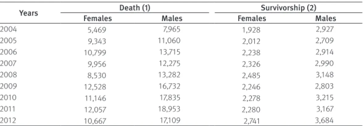
Table 1 shows exposed individuals of Graph 1 in greater detail, classiied by sex and type of insurance coverage: death (pertaining to risk products) and survivorship (pertaining to old-age pensions and savings products). In our analysis, all individuals who have both coverages are considered to belong to the survivorship group only. As one can see in section 4, mortality tables for these groups show a clear separation between death and survivorship coverages. Table 1 also shows that death coverage accounts for more than four times as many individuals as survivorship coverage.
TABLE 1
Insured population by type of insurance coverage and sex (/1,000) Brazil – 2004-2012
Years Death (1) Survivorship (2)
Females Males Females Males
2004 5,469 7,965 1,928 2,927
2005 9,343 11,060 2,012 2,709
2006 10,799 13,715 2,238 2,914
2007 9,956 12,275 2,326 2,990
2008 8,530 13,282 2,485 3,148
2009 12,528 16,732 2,246 2,803
2010 11,146 17,835 2,278 3,215
2011 12,057 18,953 2,280 3,167
2012 10,667 17,109 2,741 3,684
Source: Brazilian insurance companies participating in the analysis. (1) Risk products.
(2) Old-age pensions.
Regarding territorial distribution of the studied population, the total number of individuals in the ive geographical regions of Brazil is shown in Table 2. Notice that more than 70 per cent of the population belongs to the most socioeconomically developed regions, the South and Southeast, where about 28 per cent of the population participates in the insurance market (Note: the data represent about 80 per cent of the Brazilian insurance market). It can also be inferred that the Brazilian insured population corresponds to around 22 per cent of the entire Brazilian population in 2012, which is a small proportion compared to more developed countries.
TABLE 2
Insured and general population by region and type of insurance coverage (/1,000) Brazil – 2012
Zones Death (1) Survivorship (2) Both coverages Brazilian population
N % N % N % N %
Southeast 14,319 51 3,973 61 18,292 53 81,566 42
South 5,164 19 1,081 17 6,245 18 27,732 15
Northeast 4,849 17 783 12 5,632 17 53,907 28
Central-West 2,329 8 430 7 2,759 8 14,424 7
North 1,237 5 195 3 1,432 4 16,318 8
Total 27,897 100 6,462 100 34,359 100 193,947 100
Source: Brazilian insurance companies participating in the analysis; IBGE. Censo Demográico 2010. (1) Risk products.
Graph 3 shows the population under study for the year 2012 distributed by age and sex. Almost three-fourths of this population is concentrated between the ages of 20 and 50, and the maximum number of deaths is at age 58 for males and 62 for females. The decrease at ages 82 and over is due to the much smaller number of insured elderly people.
GRAPH 3
Distribution of number of insured individuals and deaths by age and sex Brazil – 2012
0 500 1,000 1,500 2,000 2,500
0 50,000 100,000 150,000 200,000 250,000 300,000 350,000 400,000 450,000 500,000
0 5 10 15 20 25 30 35 40 45 50 55 60 65 70 75 80 85 90 95 100
I
Individuals
Age
Females Males Female deaths Male deaths
Deaths
Source: Brazilian insurance companies participating in the analysis, CNIS, and SISOBI.
Table 3 shows the distribution of the Brazilian insured population under study for all years, highlighting the very low igures regarding the extreme age groups (i.e., young and old individuals). This is particularly true for the age 80 or above, which, as we shall see in the next section, is essential for completion of the table.
TABLE 3
Number of insured individuals at young and old ages (/1,000) Brazil – 2004-2012
Years
Age 18 years Age 60 years Age 80 years
Males Females Males Females Males Females
N % N % N % N % N % N %
2004 285 2.6 240 3.3 946 8.7 704 9.5 48 0.4 31 0.4
2005 385 2.8 336 3.0 1,194 8.7 1,202 10.6 67 0.5 63 0.6
2006 444 2.7 390 3.0 1,571 9.4 1,529 11.7 105 0.6 98 0.8
2007 477 4.4 406 5.9 929 8.5 676 9.8 65 0.6 52 0.8
2008 510 3.8 439 5.1 1,242 9.3 915 10.7 87 0.7 75 0.9
2009 459 2.5 397 3.0 1,622 9.0 1,360 10.3 90 0.5 75 0.6
2010 535 2.5 446 3.3 2,048 9.7 1,612 12.0 134 0.6 104 0.8
2011 612 2.8 511 3.6 2,842 12.8 2,382 16.6 214 1.0 200 1.4
2012 649 3.1 568 4.2 2,921 14.0 2,486 18.5 246 1.2 246 1.8
Total 4,355 3.0 3,734 3.7 15,315 10.4 12,865 12.7 1,055 0.7 944 0.9
Methodology for computing the mortality tables
Annual mortality rates
Data provided by insurance companies still contained inaccuracies and inconsistencies even ater correction using data from CNIS/SISOBI. The set of problematic data needed
to be iltered out using reliable criteria. In this section, procedures used to ilter data and
compute crude mortality rates corresponding to the years 2007-2012 are detailed. Part of these procedures is also described in (DE OLIVEIRA et al., 2012a).
First, clearly inconsistent records were discarded, such as those containing: • Invalid CPF, date of birth or death;
• Wildcard CPF (i.e., CPF shared by more than four diferent individuals in the database); • Date of death preceding the beginning of the insurance contract or birth date.
Second, individuals were sorted into diferent subpopulations, which are deined as groups of individuals with the same sex, coverage (death or survivorship), insurance company, and acquired insurance product, in the same calendar year. This grouping was necessary because there is a clear separation between the mortality tables for males and females, and also between individuals with diferent coverages of the same sex. Additionally, it allows iltering out inconsistent data records and unbalanced insurance products in a more precise way, since the same company may report problematic data for some products but not others.
Next, the subpopulations were statistically iltered in order to exclude outliers (which may correspond to problematic data). This iltering method only makes sense for statistically relevant groups; for this reason, subpopulations with fewer than 1000 individuals were discarded. Each remaining subpopulation was then grouped by sex and coverage, and with similar subpopulations from the past two calendar years (e.g., to ilter the subpopulations corresponding to the annual table of 2008, subpopulations of 2006 and 2007 were also taken into consideration). This was done to avoid large gaps between annual tables for consecutive years.
In order to compare these subpopulations and ilter out those with too many or too few death records, two extreme mortality tables were used as a basis of comparison, namely: • IBGE Complete Mortality Tables 2005, based on mortality in Brazil’s general popu-lation in 2005, which has higher mortality rates than the Brazilian insured popula-tion (IBGE, 2005). This table was continuously extended to 103 years for use in the iltering process.
• CSO 2001 Valuation Basic Table, which has low mortality rates, based on some US insurance companies’ 1990-1995 mortality experience , projected to 2001 (AMERICAN ACADEMY OF ACTUARIES, 2002).
For each subpopulation s, the ratio between the observed and the theoretical number
, ,
, ,
∑
=r o
q E s e
s e x s x
x
( 1 )
where os is the total observed number of death records of subpopulation s, qe,x is the
probability of death at age x in extreme table e, and Es,x denotes the number of individuals at age x in subpopulation s. When rs,e is close to 1, this means that the mortality rate of
subpopulation is close to the rate of extreme table e.
If all subpopulations have about the same mortality pattern, then all values of rs,e should be roughly near a central value and close to each other. Subpopulations with rs,e very diferent from the central value should be discarded, as they probably involve data errors. Since the
numerator of each fraction rs,e is the actual number of deaths for each subpopulation, and
since the number of deaths, considered as a random variable, is the sum of independent binomial random variables (one for each age), one may assume that the numerator of each fraction will be approximately normally distributed. As such, Tukey’s fences (TUKEY, 1977) were applied to the ratios rs,e in order to deine and discharge outlier subpopulations, via an iterative process that was repeated until all outliers ceased to exist. For the present case, each bound was established by adding and subtracting 1.5 inter-quartile distances from the median, leaving roughly 95 per cent of the subpopulations unafected.
Ater this statistical iltering, the remaining subpopulations were further examined, in order to visually detect and discard those for which mortality rates greatly diverged from the expected mortality pattern for human populations. Graph 4 shows an example of an insurance company/product subpopulation that was excluded from the inal population due to its over mortality with respect to the IBGE 2005 table, and its non-increasing mortality rates over the age interval from 20 to 65 years, which is not an expected mortality pattern. This indicates a likely error in the death records.
GRAPH 4
Example of an excluded subpopulation in the data iltering process
0,00001 0,0001 0,001 0,01 0,1 1
0 5 10 15 20 25 30 35 40 45 50 55 60 65 70 75 80 85 90 95 100
Excluded subpopulation CSO 2001 VBT IBGE 2005
Mortality rate
Age
Graph 1 shows the extent of this data iltering process for each year from 2004 to 2012. It shows the great impact iltering has on the amount of data used for the construction of BR-EMS tables. For instance, in 2012 approximately 34 per cent of individuals were discarded due to data iltering.
Ater all subpopulations were iltered, the death probability qc s x, ,
y
for year y for the
population with coverage c and sex s at age x was estimated by the mortality rate, as follows:
ˆ, , , , ,
, , =
q d
E c s x y c s x
y
c s x y
(2)
where dc s xy, , is the total number of deaths and Ec s xy, , is the total exposition (i.e., respectively
the sum of deaths and exposition of all remaining subpopulations with coverage c and sex
s of calendar year y).
BR-EMS 2015 tables
The procedure detailed in the previous section was used to obtain annual mortality rates ˆ, ,
qc s xy for the years 2007 to 2012. For each coverage c and sex s, the crude mortality rates
of BR-EMS 2015 tables, ˆ
, , 15
qc s xBR , were then estimated as an exponentially weighted average
of ˆ , ,
qc s xy and the corresponding BR-EMS 2010 table entry ˆ
, , 10
qc s xBR , namely,
qc s xBR qc s x qc s x qc s x qc s x qc s x qc s x qc s x BR = + + + + + + ˆ ˆ 2 ˆ 4 ˆ 8 ˆ 16 ˆ 32 ˆ 64 , , ,
15 , ,
2012 , , 2011 , , 2010 , , 2009 , , 2008 , , 2007 , , 10 (3)
This weighting emphasizes the most recent information, because the most current value ˆ
, , 2012
qc s x has the same weight as all past tables combined.
The resulting rates were graduated by applying diferent methods to three distinct age groups, hereater called “younger”, “intermediate”, and “older”. The 2010 and 2015 versions of the tables difer on this point, as BR-EMS 2010 only had the Heligman-Pollard model applied to its full set of ages, from the earliest to the oldest. The separation into three age groups was necessary due to the relative scarcity of data for the younger group (as seen in Graph 3 and Table 3), and to the well-known death undercounting in the older group, as reported in Gomes and Turra (2009) and Queiroz and Sawyer (2012). More extensive modelling was required for these two groups, whereas the crude rates of the intermediate age interval exhibit smooth behaviour. The exact range of each age group by coverage and sex are:
• Death coverage, females. Younger: 19 and under; Intermediate: 20-99; Older: 100 and over.
• Death coverage, males. Younger: 16 and under; Intermediate: 17-90; Older: 91 and over.
• Survivorship coverage, females. Younger: 17 and under; Intermediate: 18-100; Older: 101 and over.
For the younger group, crude rates ˆ , ,
qc s xy were graduated by a nonlinear it to the data using a nine-parameter version of the Heligman-Pollard model (HELIGMAN; POLLARD, 1980),
( )
1
( ) (In In )2
= + +
+
+ − −
q x A De GH
KGH
x B E x F x
x
C
(4)
Due to the scarcity of data in this age interval, the sets of both death and survivorship coverage were used together to obtain the parameters.
For the intermediate group, in which most of the exposed population is concentrated, the rates qc s x, , were obtained by a simple moving average of length three of ˆ
, ,
qc s x, followed by one of length ive for further smoothing. There was no need for more extensive modelling due to the amount of good quality data available for this age group – all resulting rates are fairly smooth and monotone for this age interval, with the exception of naturally occurring humps around age 23. Rates for younger ages were then smoothly interpolated to the intermediate rates using a suggestion proposed by (BRASS, 1975), calculating a constant logit distance between the curves for males and females.
The older group had its rates qc s x, , generated from exponential extrapolations of the intermediate group rates. Any two diferent curves were forced to coincide at the age where they irst met. Thus, rates for males insured under death and survivorship coverages coincide from 97 years on; rates for females insured under death coverage coincide with the two rates for males from 100 years on; and the rates for females insured under survivorship coverage coincide with the remaining rates from 117 years on.
Conidence intervals
Assuming that all individuals with the same age x die independently and with the same
probability, the number of deaths in year y for coverage c and sex s, dc s xy, ,, can be understood
as a random variable with a binomial B E(| c s xy, , |,qc s xy, , ) distribution, where qc s xy, , is unknown. As before, let qˆc s xy, , =dc s xy, , /Ec s xy, ,. Using the binomial hypothesis, and estimating qc s xy, , with ˆ
, ,
qc s xy , one has the following estimate for the variance of ˆ , ,
qc s xy :
Var (ˆ, , ) ˆ, , (1 ˆ, , ) , ,
= −
q q q
E c s x
y c s x y
c s x y
c s x y
(5)
For a given age x, each annual rate ˆ , ,
qc s xy is assumed to be independent from the others;
therefore, the variance of ˆ
, , 15
qc s xBR can be estimated by the weighted sum of the variances of ˆ
, ,
qc s xy and ˆ
, , 10
qc s xBR (cf. Eq. 2),
Var (ˆ ) Var (ˆ )
2
Var (ˆ )
4
Var (ˆ ) Var (ˆ )
64 , ,
15 , ,
2012 2 , , 2011 2 , , 2007 , , 10 2 ⋯ = + + + +
qc s xBR qc s x qc s x qc s x qc s x BR
(6)
Finally, using the normal approximation to ˆ
, , 15
qc s xBR , one gets the conidence interval
q q
− +
qˆ, ,15 1.96 Var( ˆq , ,15), ˆ, ,15 1.96 Var( ˆ, ,15)
c s x BR
c s x BR
c s x BR
c s x BR
The mortality tables
In this section, BR-EMS 2015 tables are presented for both sexes and the two diferent types of insurance coverage: death and survivorship. The complete tables are given in Appendix A (TABLES 1 to 4), following the oicial nomenclatures as (SUPERINTENDÊNCIA DE SEGUROS PRIVADOS, 2015):
• Death coverage, females: BR-EMSmt-V.2015-f. • Death coverage, males: BR-EMSmt-V.2015-m. • Survivorship coverage, females: BR-EMSsb-V.2015-f. • Survivorship coverage, males: BR-EMSsb-V.2015-m.
Graph 5 presents the case of males insured under death coverage. The crude rates qˆ are
shown along with the smoothed curve qx obtained by the graduation techniques described
in section 3. Note that conidence intervals between ages 20 to 90 are very tight, reflecting the large amount of data available, supporting the use of moving averages instead of the Heligman-Pollard model in the intermediate interval.
GRAPH 5
BR-EMS 2015 mortality table for the Brazilian insured population, along with crude mortality rates, and conidence intervals for males, death coverage (on logarithmic scale)
Brazil – 2015
0,00001 0,0001 0,001 0,01 0,1 1
0 5 10 15 20 25 30 35 40 45 50 55 60 65 70 75 80 85 90 95 100 105 110 115
Mortality rate
Age 0,0001
0,001 0,01 0,1 1
qx BR-EMSmt-V.2015-m -IC(95%) +IC(95%)
Source: Brazilian insurance companies participating in the analysis, CNIS, and SISOBI.
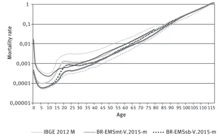
Graph 6 shows all four cases together with IBGE 2012 tables for the sake of comparison. One clearly notices the separation between males and females. Overmortality for males is plainly observed in both coverages, mainly around age 20, where there is a more pronounced hump in the curve due to deaths from external causes. Note that rates for death coverage are higher than rates for survivorship coverage for males and females at all ages.
GRAPH 6
BR-EMS 2015 mortality tables for the Brazilian insured population alongside the IBGE Complete Mortality Tables 2012 for the Brazilian general population (on logarithmic scale)
0,00001 0,0001 0,001 0,01 0,1 1
0 5 10 15 20 25 30 35 40 45 50 55 60 65 70 75 80 85 90 95 100 105 110 115
Age
Mortality rate
IBGE 2012 M BR-EMSmt-V.2015-m BR-EMSsb-V.2015-m
IBGE 2012 F BR-EMSmt-V.2015-f BR-EMSsb-v.2015-f
Source: IBGE: Complete Mortality Tables, 2012; Brazilian insurance companies participating in the analysis, CNIS, and SISOBI.
GRAPH 7
Comparison between the 2010 and 2015 versions of the BR-EMS tables for the Brazilian insured population, death coverage (on logarithmic scale)
0,00001 0,0001 0,001 0,01 0,1 1
0 5 10 15 20 25 30 35 40 45 50 55 60 65 70 75 80 85 90 95 100 105 110 115
BR-EMSmt-V.2010-f BR-EMSmt-V.2015-f
BR-EMSmt-V.2010-m BR-EMSmt-V.2015-m Age
Mortality rate
Source: Brazilian insurance companies participating in the analysis, CNIS, and SISOBI.
GRAPH 8
Comparison between the 2010 and 2015 versions of the BR-EMS tables for the Brazilian insured population, survivorship coverage (on logarithmic scale)
0,00001 0,0001 0,001 0,01 0,1 1
0 5 10 15 20 25 30 35 40 45 50 55 60 65 70 75 80 85 90 95 100 105 110 115
BR-EMSsb-V.2010-f BR-EMSsb-V.2015-f
BR-EMSsb-V.2010-m BR-EMSsb-V.2015-m
Age
Mortality rate
Source: Brazilian insurance companies participating in the analysis, CNIS, and SISOBI.
TABLE 4
Life expectation of the population under survivorship coverage according to the BR-EMS 2015 tables, and that of the Brazilian population according to IBGE 2012 tables, at ages 0, 30 and 60 (in years)
Sex Age IBGE 2012 BR-EMS 2015Survivorship BR-EMS 2015 and IBGE 2012Diference between
Females
0 78.3 87.8 9.5
30 50.3 58.1 7.8
60 23.3 29.5 6.2
Males
0 71 82.4 11.4
30 44.4 53 8.6
60 19.8 25.1 5.3
Source: IBGE. Complete Mortality Tables, 2012; Brazilian insurance companies participating in the analysis, CNIS, and SISOBI.
GRAPH 9
Comparison of the overmortality for males between the 2010 and 2015 versions of the BR-EMS mortality tables for the Brazilian insured population (on logarithmic scale)
0
0,5 1 1,5 2 2,5 3 3,5 4
20 25 30 35 40 45 50 55 60 65 70 75 80 85 90
Death coverage 2010 Death coverage 2015 Survivorship coverage 2010 Survivorship coverage 2015
Overmortality
Age
Source: Brazilian insurance companies participating in the analysis, CNIS, and SISOBI.
Comparison with other mortality tables
In order to highlight some characteristics of the Brazilian insured population under analysis, we performed some comparisons with foreign market tables, as well as with general population tables from developed countries. In Graph 10 illustrates the AT 2000 and RV-2009 tables in direct comparison with the survivorship version of BR-EMS 2015 for males. RV-2009 was constructed using the experience of the Chilean annuity market, pension funds, and the Social Security Institute (SUPERINTENDENCIA DE PENSIONES, 2010), while AT 2000 (JOHANSEN, 1995) uses data from the American individual annuity market and was the former standard for the Brazilian market before the appearance of BR-EMS 2010. Note the similarity of the BR-EMS 2015 with the AT-2000 at most of the age intervals under consideration and, similarly, its lower mortality against the Chilean RV-2009.
GRAPH 10
Comparison between the BR-EMS 2015 table for males/survivorship coverage with other market tables
0,00001 0,0001 0,001 0,01 0,1 1
0 5 10 15 20 25 30 35 40 45 50 55 60 65 70 75 80 85 90 95 100 105 110 115
BR-EMS-2015 RV-2009 (Chile) AT-2000 (USA)
Mortality rate
Age
Sources: Brazilian insurance companies participating in the analysis, CNIS, and SISOBI; Superintendencia de Pensiones, Chile: Circular n. 1679/2010; Society of Actuaries, USA: Mortality and Other Rate Tables, 2016.
GRAPH 11
Comparison between the BR-EMS 2015 table for males/death coverage with foreign tables (UK and USA)
0,00001 0,0001 0,001 0,01 0,1 1
0 5 10 15 20 25 30 35 40 45 50 55 60 65 70 75 80 85 90 95 100 105
BR-EMS-2015 USA (2013) UK (2013)
Age
Mortality rate
Conclusions
This paper describes the database and procedures used to construct BR-EMS mortality tables, which were the irst ones compiled from Brazilian market experience data. Despite being more focused on the 2015 version, this paper also contains an account of the design of BR-EMS 2010 via a direct comparison between the two versions. For instance, the newer version showed improvements with regards to the amount and quality of collected data from the participating insurance companies.
The database contains over a billion records, from which information on around 83 million insured individuals was compiled, allowing the elaboration of four distinct tables, classiied under sex and insurance coverage types (death or survivorship). The whole database has been scrutinized and checked against oicial government social information databases, which proved to be a necessary step for the accuracy of a large part of the collected data.
For the construction of BR-EMS 2010 and 2015 tables, data were irst classiied into subpopulations separated by calendar year, company, product, sex, and type of insurance coverage. These subpopulations were iltered using various exclusion criteria, ranging from possessing a small number of individuals to having a nonstandard mortality pattern. Aterwards, outliers were further excluded using Tukey’s fences. The remaining groups of subpopulations were merged, giving rise to the inal population from which all death rates were obtained. The Heligman–Pollard model was then used to graduate the set of obtained rates; however, distinctly from BR-EMS 2010, which was entirely itted with this model, the 2015 version used parametric models only at the extreme age groups. In the range between 18 and 90 years, only moving averages were used, due to the smooth behaviour exhibited by crude rates in this interval.
Mortality tables for the Brazilian insured population were shown to be much lower than those for the Brazilian general population, and more akin to those for more developed countries, such as the USA and UK. This reflects the fact that only about 22 per cent of the Brazilian population – which can be assumed to have a higher socioeconomic level compared to the rest of the population – has some kind of insurance contract.
As future studies, we cite the investigation of mortality trends at older ages, which will depend on insurance companies providing further and more speciic; analysis of mortality rates in diferent regions of Brazil, which may improve insurance companies’ underwriting experience; and analysis of the changes in mortality rates for the Brazilian insured population over the years.
References
BRASS, W. Methods for estimating fertility and mortality from limited and defective data. Chapel Hill: University of North Carolina, 1975.
DUCHÈNE, J.; WUNSCH, G. J. Population aging and the limits to human life. Louvain-la-Neuve: CIACO, 1988.
GOMES, M. M. F.; TURRA, C. M. The number of centenarians in Brazil: indirect estimates based on death certiicates. Demographic Research, v. 20, p. 493-502, 2009.
HELIGMAN, L.; POLLARD, J. H. The age pattern of mortality. Journal of the Institute of Actuaries, v. 107, p. 49-80, 1980.
IBGE – Instituto Brasileiro de Geograia e Estatística. Censo Demográico: microdados. Rio de Janeiro: IBGE, 2010.
_________. Complete life tables 2005. Available at: <http://www.ibge.gov.br/english/estatistica/ populacao/tabuadevida/2005/default.shtm>. Accessed on: 1 Dec. 2016.
_________. Complete mortality tables 2012. Available at: <http://www.ibge.gov.br/english/ estatistica/populacao/tabuadevida/2012/default.shtm>. Accessed on: 1 Dec. 2016.
JOHANSEN, R. J. Review of adequacy of 1983 individual annuity mortality table. Transactions of Society of Actuaries, v. 47, p. 211-249, 1995.
MCCULLAGH, P.; NELDER, J. A. Generalized linear models. London: Chapman and Hall, 1989. NATIONAL CENTER FOR HEALTH STATISTICS. Multiple cause of death public use ile, 2006. USA, 2013. Available at: <http://www.mortality.org>. Accessed on: 1 Dec. 2016.
NELDER, J. A.; WEDDERBURN, R. W. Generalized linear models. Journal of the Royal Statistical Society A, v. 135, n. 3, p. 370-384, 1972.
OFFICE FOR NATIONAL STATISTICS, UK. Deaths by sex and single year of age until the last age 110+. 2013. Available at: <http://www.mortality.org> Accessed on: 1 Dec. 2016.
DE OLIVEIRA, M.; FRISCHTAK, R.; RAMIREZ, M.; BELTRÃO, K.; PINHEIRO, S. Brazilian mortality and survivorship life tables: insurance market experience – 2010. Rio de Janeiro: Fundação Escola Nacional de Seguros – Funenseg, 2012.
_________. Tábuas biométricas de mortalidade e sobrevivência: experiência do mercado segurador brasileiro – 2010. Rio de Janeiro: Fundação Escola Nacional de Seguros – Funenseg, 2012.
QUEIROZ, B. L.; SAWYER, D. O. O que os dados de mortalidade do Censo de 2010 podem nos dizer? Revista Brasileira de Estudos de População, v. 29, n. 2, p. 225-38, 2012.
SOCIETY OF ACTUARIES. Mortality and other rate tables. USA, 2016. Available at: <http://mort. soa.org/>. Accessed on: 1 Dec. 2016.
SUPERINTENDENCIA DE PENSIONES. Circular n. 1679/2010. Chile, 2010. Available at: <http:// www.spensiones.cl/iles/normativa/circulares/CAFP1679.pdf>. Accessed on: 1 Dec. 2016. SUPERINTENDÊNCIA DE SEGUROS PRIVADOS. Circular SUSEP n. 402, de 18 de março de 2010.
Diário Oicial da União, Brasília, v. 53, p. 30, 2010.
_________. Circular SUSEP n. 515, de 3 de julho de 2015. Diário Oicial da União, Brasília, v. 133, p. 23-25, 2015.
TUKEY, J. W. Exploratory data analysis. Reading: Addison-Wesley Publishing Company, 1977.
About the authors
Mário Moreira Carvalho de Oliveira has doctorate degree in Dynamic Systems, University of
Warwick. Professor of the Applied Mathematics Department of Universidade Federal do Rio
de Janeiro (UFRJ) and head of the Applied Mathematics Laboratory of UFRJ.
Milton Ramos Ramirez has doctorate degree in Systems and Computational Engineer from
Universidade Federal do Rio de Janeiro (UFRJ). Professor of the Applied Mathematics
Department of Universidade Federal do Rio de Janeiro (UFRJ) and vice-head of the Applied Mathematics Laboratory of UFRJ.
Ricardo Milton Frischtak researcher of the Applied Mathematics Department of Universidade
Federal do Rio de Janeiro (UFRJ).
Rafael Brandão de Rezende Borges has doctorate degree in Mathematics from Universidade
Federal do Rio de Janeiro (UFRJ). Professor of the Mathematical Analysis Department of
Universidade do Estado do Rio de Janeiro (UERJ) and researcher of the Applied Mathematics
Laboratory of UFRJ.
Bruno Costa has doctorate degree in Applied Mathematics from University of Indiana Professor
of the Applied Mathematics Department of Universidade Federal do Rio de Janeiro (UFRJ) and researcher of the Applied Mathematics Laboratory of UFRJ.
Ricardo Cunha Pedroso has undergraduation degree in Actuarial Sciences and Statistics from
Universidade Federal do Rio de Janeiro (UFRJ). Researcher of the Applied Mathematics
Laboratory of UFRJ.
Contact address (all authors)
Av. Athos da Silveira Ramos 149, Sala ABC-110
Centro de Tecnologia, Cidade Universitária, Ilha do Fundão 21941-909 – Rio de Janeiro-RJ, Brasil
Resumo
Tábuas de mortalidade para a população brasileira de segurados
Este artigo descreve a construção das tábuas de mortalidade BR-EMS 2015 para a população brasileira de segurados. As tábuas foram elaboradas a partir de dados coletados de companhias de seguros que representam 80% do mercado segurador brasileiro e são atualizações das tábuas BR-EMS 2010, que foram as primeiras tábuas de mortalidade a serem produzidas usando-se a experiência do mercado segurador brasileiro. Informações adicionais de fontes governamentais foram utilizadas para complementar e melhorar as informações fornecidas pelas companhias de seguros. As taxas de mortalidade da população contratante de produtos com cobertura de morte são notavelmente diferentes daquelas referentes aos contratantes de produtos de sobrevivência. Assim, quatro tábuas de mortalidade diferentes foram construídas, separando a população por sexo e também pelo tipo de cobertura de seguro. Uma comparação direta entre as tábuas BR-EMS 2015 com as estatísticas da população brasileira geral mostra uma diferença considerável nas expectativas de vida. As tábuas BR-EMS 2015 ainda são comparadas com outras tábuas de mortalidade.
Resumen
Tablas de mortalidad de la población brasileña asegurada
En este trabajo se describe la construcción de las tablas de mortalidad BR-EMS 2015 para la población asegurada de Brasil. Las tablas se confeccionaron a partir de datos recogidos de las compañías de seguros que representan alrededor del 80% del mercado brasileño de seguros y son actualizaciones de sus versiones anteriores, BR-EMS 2010 —las primeras tablas de mortalidad hechas con base en la experiencia del mercado brasileño—. Se utilizó información adicional de fuentes gubernamentales para complementar y mejorar las bases de datos de las empresas. Las tasas de mortalidad de la población con contrato de productos de riesgo (cobertura de la muerte) son notablemente diferentes a las de los incluidos en los productos de ahorro (cobertura de supervivencia). Por lo tanto, cuatro diferentes tablas de mortalidad se han construido, separando la población según el sexo y el tipo de cobertura de seguro. Una comparación directa entre las tablas BR-EMS 2015 para la población asegurada de Brasil con las estadísticas de la población en general de Brasil muestra una diferencia considerable en la esperanza de vida. Las tablas BR-EMS 2015 también se comparan con otras tablas de vida.
Palabras clave: Tablas actuariales. Mortalidad. Índice de mortalidad. Mercado de seguros. Heligman-Pollard.
Appendix
BR-EMS 2015 mortality tables
TABLE 1
BR-EMS 2015 mortality table for males, survivorship coverage
BR-EMSsb-V.2015-m
Age x qx -IC(95%) +IC(95%) ex Age x qx -IC(95%) +IC(95%) ex
0 0.0003372 – 0.0004601 82.4 60 0.0060008 0.0055785 0.0065806 25.1
1 0.0001568 0.0000313 0.0003004 81.4 61 0.0065038 0.0057443 0.0068260 24.3
2 0.0000941 0.0000019 0.0001312 80.4 62 0.0070974 0.0063579 0.0075268 23.4
3 0.0000688 – 0.0001466 79.4 63 0.0078021 0.0068684 0.0081651 22.6
4 0.0000582 0.0000101 0.0001562 78.4 64 0.0086713 0.0076143 0.0090447 21.8
5 0.0000543 – 0.0001123 77.4 65 0.0095833 0.0089048 0.0105576 21.0
6 0.0000539 0.0000287 0.0001895 76.4 66 0.0105349 0.0096438 0.0114647 20.2
7 0.0000555 0.0000197 0.0001732 75.5 67 0.0114564 0.0110306 0.0130871 19.4
8 0.0000584 0.0000200 0.0001495 74.5 68 0.0124987 0.0107566 0.0128659 18.6
9 0.0000624 0.0000020 0.0001252 73.5 69 0.0135974 0.0120266 0.0143593 17.8
10 0.0000673 0.0000100 0.0001456 72.5 70 0.0150356 0.0131070 0.0156831 17.1
11 0.0000738 0.0000257 0.0001844 71.5 71 0.0166761 0.0151923 0.0181320 16.3
12 0.0000831 0.0000425 0.0002255 70.5 72 0.0187002 0.0162117 0.0193218 15.6
13 0.0000971 0.0000089 0.0001312 69.5 73 0.0208752 0.0197566 0.0233805 14.9
14 0.0001182 0.0000188 0.0001508 68.5 74 0.0232898 0.0204555 0.0242138 14.2
15 0.0001487 0.0000634 0.0002945 67.5 75 0.0257844 0.0237511 0.0279666 13.5
16 0.0001909 0.0000195 0.0001965 66.5 76 0.0286674 0.0263564 0.0310054 12.8
17 0.0002796 0.0001060 0.0003647 65.5 77 0.0317212 0.0279893 0.0330158 12.2
BR-EMSsb-V.2015-m
Age x qx -IC(95%) +IC(95%) ex Age x qx -IC(95%) +IC(95%) ex
19 0.0004909 0.0003343 0.0006625 63.6 79 0.0382344 0.0369938 0.0433616 11.0
20 0.0006045 0.0005644 0.0009935 62.6 80 0.0417852 0.0377950 0.0445176 10.4
21 0.0007069 0.0004186 0.0007494 61.6 81 0.0457989 0.0388412 0.0458777 9.8
22 0.0007623 0.0007485 0.0011770 60.7 82 0.0499480 0.0481660 0.0566452 9.3
23 0.0007817 0.0007073 0.0010812 59.7 83 0.0544018 0.0473654 0.0564657 8.7
24 0.0007731 0.0004720 0.0007466 58.8 84 0.0597001 0.0555617 0.0660344 8.2
25 0.0007544 0.0006772 0.0009975 57.8 85 0.0665090 0.0590970 0.0710866 7.7
26 0.0007373 0.0005705 0.0008389 56.9 86 0.0744187 0.0581873 0.0710348 7.2
27 0.0007298 0.0005357 0.0007748 55.9 87 0.0839599 0.0775002 0.0938849 6.8
28 0.0007258 0.0006692 0.0009324 54.9 88 0.0934390 0.0884822 0.1085387 6.3
29 0.0007177 0.0006331 0.0008741 54.0 89 0.1049700 0.0882675 0.1108556 5.9
30 0.0007211 0.0005669 0.0007785 53.0 90 0.1143591 0.1084554 0.1372477 5.6
31 0.0007342 0.0005625 0.0007703 52.0 91 0.1247292 0.0944340 0.1261158 5.2
32 0.0007579 0.0006251 0.0008474 51.1 92 0.1325577 0.1340578 0.1764087 4.9
33 0.0007941 0.0006910 0.0009280 50.1 93 0.1466181 0.1017761 0.1465084 4.6
34 0.0008395 0.0007406 0.0009804 49.2 94 0.1585720 0.1310846 0.1887968 4.3
35 0.0008802 0.0007860 0.0010373 48.2 95 0.1737468 0.1202828 0.1882540 4.0
36 0.0009202 0.0007437 0.0009856 47.2 96 0.1895589 0.1800968 0.2786733 3.7
37 0.0009512 0.0008456 0.0011122 46.3 97 0.2053710 0.1280817 0.2399470 3.4
38 0.0009876 0.0008457 0.0011124 45.3 98 0.2220684 0.1372591 0.2704877 3.2
39 0.0010291 0.0009099 0.0011870 44.4 99 0.2401233 0.0936042 0.2478258 3.0
40 0.0010883 0.0008832 0.0011552 43.4 100 0.2596462 0.0709706 0.2612205 2.8
41 0.0011563 0.0009721 0.0012590 42.5 101 0.2807563 – – 2.6
42 0.0012443 0.0010892 0.0013957 41.5 102 0.3035828 – – 2.4
43 0.0013505 0.0011953 0.0015121 40.6 103 0.3282651 – – 2.2
44 0.0014798 0.0012633 0.0015954 39.6 104 0.3549543 – – 2.0
45 0.0016034 0.0014090 0.0017597 38.7 105 0.3838133 – – 1.9
46 0.0017246 0.0015799 0.0019457 37.7 106 0.4150187 – – 1.7
47 0.0018463 0.0017713 0.0021654 36.8 107 0.4487611 – – 1.6
48 0.0020009 0.0016472 0.0020233 35.9 108 0.4852470 – – 1.4
49 0.0021789 0.0018339 0.0022444 34.9 109 0.5246993 – – 1.3
50 0.0023873 0.0020945 0.0025436 34.0 110 0.5673592 – – 1.2
51 0.0026229 0.0024889 0.0029863 33.1 111 0.6134875 – – 1.1
52 0.0029034 0.0026636 0.0031939 32.2 112 0.6633662 – – 1.0
53 0.0032172 0.0027495 0.0033021 31.3 113 0.7173002 – – 0.9
54 0.0035536 0.0031244 0.0037195 30.4 114 0.7756192 – – 0.8
55 0.0039070 0.0036191 0.0042868 29.5 115 0.8386798 – – 0.7
56 0.0042981 0.0040578 0.0047995 28.6 116 0.9068674 – – 0.6
57 0.0047163 0.0042631 0.0050350 27.7 117 0.9805989 – – 0.5
58 0.0051323 0.0045029 0.0053273 26.9 118 1.0000000 – – 0.5
59 0.0055507 0.0052183 0.0061402 26.0
TABLE 2
BR-EMS 2015 mortality table for females, survivorship coverage
BR-EMSsb-V.2015-f
Age x qx -IC(95%) +IC(95%) ex Age x qx -IC(95%) +IC(95%) ex
0 0.0003438 – 0.0005157 87.8 60 0.0033009 0.0028676 0.0037850 29.5
1 0.0001527 0.0000024 0.0002489 86.8 61 0.0035957 0.0028336 0.0038094 28.6
2 0.0001159 0.0000291 0.0002981 85.8 62 0.0039135 0.0034820 0.0046102 27.7
3 0.0000791 – 0.0001047 84.8 63 0.0042898 0.0036846 0.0049342 26.8
4 0.0000576 0.0000272 0.0002201 83.9 64 0.0047135 0.0038296 0.0050806 25.9
5 0.0000494 0.0000895 0.0003281 82.9 65 0.0052346 0.0043106 0.0057349 25.0
6 0.0000471 0.0000358 0.0002272 81.9 66 0.0057864 0.0050778 0.0067244 24.1
7 0.0000475 0.0000894 0.0003290 80.9 67 0.0063930 0.0052629 0.0069876 23.3
8 0.0000496 0.0000050 0.0001481 79.9 68 0.0071061 0.0064645 0.0084680 22.4
9 0.0000526 0.0000120 0.0001408 78.9 69 0.0079214 0.0064644 0.0085299 21.6
10 0.0000565 – 0.0000802 77.9 70 0.0088362 0.0068243 0.0090208 20.7
11 0.0000610 0.0000110 0.0001439 76.9 71 0.0097454 0.0093127 0.0119991 19.9
12 0.0000664 0.0000383 0.0002216 75.9 72 0.0107480 0.0093361 0.0120629 19.1
13 0.0000731 – 0.0000975 74.9 73 0.0117749 0.0103784 0.0133390 18.3
14 0.0000825 – 0.0001456 73.9 74 0.0128002 0.0106514 0.0136876 17.5
15 0.0000968 0.0000122 0.0000707 72.9 75 0.0138450 0.0122032 0.0155904 16.7
16 0.0001220 0.0000261 0.0002453 71.9 76 0.0151097 0.0135731 0.0172523 16.0
17 0.0001428 0.0001054 0.0004234 70.9 77 0.0166446 0.0134669 0.0172280 15.2
18 0.0001708 0.0000563 0.0002825 69.9 78 0.0186115 0.0159908 0.0202627 14.5
19 0.0002035 0.0000661 0.0002514 68.9 79 0.0210603 0.0179160 0.0225324 13.7
20 0.0002313 0.0000925 0.0003476 68.0 80 0.0240473 0.0200704 0.0251228 13.0
21 0.0002520 0.0001684 0.0004502 67.0 81 0.0273368 0.0251988 0.0311254 12.3
22 0.0002726 0.0001497 0.0004179 66.0 82 0.0307907 0.0274535 0.0338054 11.6
23 0.0002870 0.0001298 0.0003398 65.0 83 0.0342908 0.0312612 0.0385392 11.0
24 0.0002872 0.0002469 0.0005221 64.0 84 0.0381713 0.0334486 0.0415755 10.4
25 0.0002883 0.0001412 0.0003350 63.0 85 0.0428888 0.0358394 0.0448472 9.8
26 0.0002895 0.0001775 0.0003840 62.1 86 0.0490175 0.0403966 0.0508624 9.2
27 0.0002978 0.0001950 0.0004009 61.1 87 0.0560458 0.0474815 0.0597653 8.6
28 0.0003144 0.0001755 0.0003548 60.1 88 0.0632215 0.0575942 0.0728071 8.1
29 0.0003336 0.0002579 0.0004578 59.1 89 0.0703395 0.0669034 0.0853944 7.6
30 0.0003480 0.0002617 0.0004560 58.1 90 0.0776935 0.0664111 0.0872479 7.2
31 0.0003575 0.0003326 0.0005385 57.2 91 0.0858280 0.0660068 0.0902789 6.7
32 0.0003685 0.0002281 0.0003944 56.2 92 0.0942675 0.0765699 0.1062159 6.3
33 0.0003831 0.0002264 0.0004000 55.2 93 0.1042955 0.0870142 0.1234421 5.9
34 0.0004103 0.0003342 0.0005410 54.2 94 0.1150503 0.0986205 0.1421199 5.5
35 0.0004548 0.0002982 0.0004957 53.2 95 0.1264029 0.0941398 0.1442040 5.2
36 0.0004992 0.0004159 0.0006577 52.3 96 0.1371851 0.1101155 0.1738843 4.9
37 0.0005337 0.0004523 0.0007060 51.3 97 0.1477910 0.1075871 0.1854425 4.6
38 0.0005578 0.0004796 0.0007449 50.3 98 0.1592878 0.1059616 0.2071148 4.3
39 0.0005769 0.0004119 0.0006616 49.3 99 0.1717446 0.1126357 0.2387093 4.0
40 0.0005968 0.0003913 0.0006388 48.4 100 0.1817103 0.0899087 0.2533851 3.7
41 0.0006254 0.0005375 0.0008252 47.4 101 0.1981795 – – 3.4
42 0.0006793 0.0004663 0.0007397 46.4 102 0.2190084 – – 3.1
BR-EMSsb-V.2015-f
Age x qx -IC(95%) +IC(95%) ex Age x qx -IC(95%) +IC(95%) ex
44 0.0008159 0.0006497 0.0009733 44.5 104 0.2674637 – – 2.6
45 0.0008868 0.0007489 0.0010885 43.5 105 0.2955744 – – 2.4
46 0.0009663 0.0008232 0.0011819 42.6 106 0.3266396 – – 2.1
47 0.0010661 0.0007522 0.0011014 41.6 107 0.3609698 – – 1.9
48 0.0011670 0.0009623 0.0013619 40.7 108 0.3989082 – – 1.7
49 0.0012926 0.0010524 0.0014679 39.7 109 0.4408339 – – 1.6
50 0.0014107 0.0013033 0.0017936 38.8 110 0.4871661 – – 1.4
51 0.0015282 0.0011978 0.0016772 37.8 111 0.5383679 – – 1.2
52 0.0016306 0.0014741 0.0020170 36.9 112 0.5949510 – – 1.1
53 0.0017601 0.0014116 0.0019488 35.9 113 0.6574810 – – 1.0
54 0.0019246 0.0014128 0.0019588 35.0 114 0.7265831 – – 0.8
55 0.0021113 0.0018153 0.0024670 34.0 115 0.8029478 – – 0.7
56 0.0023298 0.0020125 0.0027104 33.1 116 0.8873386 – – 0.6
57 0.0025640 0.0023128 0.0030794 32.2 117 0.9805989 – – 0.5
58 0.0028004 0.0022189 0.0029948 31.3 118 1.0000000 – – 0.5
59 0.0030334 0.0026527 0.0035199 30.4
Source: Brazilian insurance companies participating in the analysis, CNIS, and SISOBI.
TABLE 3
BR-EMS 2015 mortality table for males, death coverage
BR-EMSmt-V.2015-m
Age x qx -IC(95%) +IC(95%) ex Age x qx -IC(95%) +IC(95%) ex
0 0.0003911 – – 79.9 60 0.0084372 0.0083931 0.0091053 23.7
1 0.0002025 – – 78.9 61 0.0092120 0.0087556 0.0095160 22.9
2 0.0001350 – – 77.9 62 0.0098629 0.0093399 0.0101625 22.1
3 0.0001068 – – 77.0 63 0.0106900 0.0102532 0.0111506 21.3
4 0.0000948 – – 76.0 64 0.0116459 0.0111312 0.0121026 20.5
5 0.0000906 – – 75.0 65 0.0125490 0.0120788 0.0131592 19.8
6 0.0000909 – – 74.0 66 0.0135129 0.0128054 0.0140171 19.0
7 0.0000938 – – 73.0 67 0.0143795 0.0138099 0.0152074 18.3
8 0.0000987 – – 72.0 68 0.0156326 0.0144610 0.0159763 17.5
9 0.0001052 – – 71.0 69 0.0167943 0.0163247 0.0180164 16.8
10 0.0001141 – – 70.0 70 0.0183789 0.0170886 0.0188987 16.1
11 0.0001277 – – 69.0 71 0.0202899 0.0189700 0.0209750 15.4
12 0.0001509 – – 68.0 72 0.0226976 0.0217824 0.0240245 14.7
13 0.0001911 – – 67.0 73 0.0254119 0.0239913 0.0264423 14.0
14 0.0002557 – – 66.0 74 0.0280659 0.0267492 0.0294820 13.4
15 0.0003486 0.0001388 0.0009397 65.1 75 0.0298929 0.0293750 0.0323556 12.7
16 0.0004682 0.0002126 0.0005339 64.1 76 0.0326954 0.0292065 0.0321888 12.1
17 0.0006352 0.0004362 0.0007509 63.1 77 0.0358784 0.0347630 0.0382833 11.5
18 0.0008963 0.0008160 0.0010616 62.2 78 0.0398857 0.0384142 0.0424148 10.9
19 0.0010702 0.0010604 0.0012523 61.2 79 0.0429656 0.0405713 0.0448674 10.4
20 0.0011606 0.0010260 0.0012046 60.3 80 0.0479174 0.0434413 0.0480848 9.8
21 0.0011614 0.0011275 0.0012927 59.3 81 0.0528419 0.0525664 0.0579730 9.3
BR-EMSmt-V.2015-m
Age x qx -IC(95%) +IC(95%) ex Age x qx -IC(95%) +IC(95%) ex
23 0.0011071 0.0010397 0.0011907 57.5 83 0.0638227 0.0597814 0.0666190 8.3
24 0.0010760 0.0009748 0.0011196 56.5 84 0.0694993 0.0668961 0.0746545 7.8
25 0.0010557 0.0009928 0.0011384 55.6 85 0.0773917 0.0702550 0.0787896 7.3
26 0.0010491 0.0009836 0.0011249 54.7 86 0.0847935 0.0818401 0.0919153 6.9
27 0.0010373 0.0009565 0.0010986 53.7 87 0.0943216 0.0872256 0.0987353 6.5
28 0.0010233 0.0009600 0.0011002 52.8 88 0.1019140 0.0963876 0.1098260 6.1
29 0.0010371 0.0009443 0.0010800 51.8 89 0.1130950 0.1019021 0.1174076 5.8
30 0.0010541 0.0009982 0.0011398 50.9 90 0.1207108 0.1171713 0.1358756 5.5
31 0.0010763 0.0010094 0.0011531 49.9 91 0.1284853 0.1152730 0.1366352 5.1
32 0.0011029 0.0010056 0.0011518 49.0 92 0.1389316 0.1199890 0.1459676 4.8
33 0.0011428 0.0010704 0.0012272 48.0 93 0.1502272 0.1399481 0.1728321 4.5
34 0.0011748 0.0011209 0.0012810 47.1 94 0.1624412 0.1568366 0.1990034 4.2
35 0.0012103 0.0010941 0.0012551 46.1 95 0.1756482 0.1542759 0.2043695 4.0
36 0.0012596 0.0011690 0.0013415 45.2 96 0.1899291 0.1410388 0.1983652 3.7
37 0.0013443 0.0012596 0.0014381 44.3 97 0.2053710 0.1422694 0.2136175 3.4
38 0.0014038 0.0013341 0.0015235 43.3 98 0.2220684 – – 3.2
39 0.0014580 0.0013409 0.0015266 42.4 99 0.2401233 – – 3.0
40 0.0015362 0.0014131 0.0016096 41.4 100 0.2596462 – – 2.8
41 0.0016430 0.0015595 0.0017676 40.5 101 0.2807563 – – 2.6
42 0.0017815 0.0016467 0.0018615 39.6 102 0.3035828 – – 2.4
43 0.0018980 0.0018131 0.0020408 38.6 103 0.3282651 – – 2.2
44 0.0020322 0.0018962 0.0021294 37.7 104 0.3549543 – – 2.0
45 0.0021748 0.0020363 0.0022776 36.8 105 0.3838133 – – 1.9
46 0.0023466 0.0022256 0.0024840 35.9 106 0.4150187 – – 1.7
47 0.0025429 0.0023953 0.0026606 34.9 107 0.4487611 – – 1.6
48 0.0027966 0.0026062 0.0028858 34.0 108 0.4852470 – – 1.4
49 0.0030327 0.0029606 0.0032710 33.1 109 0.5246993 – – 1.3
50 0.0033904 0.0030737 0.0033992 32.2 110 0.5673592 – – 1.2
51 0.0037727 0.0036405 0.0039977 31.3 111 0.6134875 – – 1.1
52 0.0042051 0.0040662 0.0044589 30.5 112 0.6633662 – – 1.0
53 0.0046575 0.0043296 0.0047377 29.6 113 0.7173002 – – 0.9
54 0.0050194 0.0049536 0.0053993 28.7 114 0.7756192 – – 0.8
55 0.0055152 0.0051148 0.0055818 27.9 115 0.8386798 – – 0.7
56 0.0059796 0.0057641 0.0062775 27.0 116 0.9068674 – – 0.6
57 0.0065447 0.0062955 0.0068442 26.2 117 0.9805989 – – 0.5
58 0.0070133 0.0067519 0.0073352 25.3 118 1.0000000 – – 0.5
59 0.0077397 0.0071131 0.0077400 24.5
TABLE 4
BR-EMS 2015 mortality table for females, death coverage
BR-EMSmt-V.2015-f
Age x qx -IC(95%) +IC(95%) ex Age x qx -IC(95%) +IC(95%) ex
0 0.0004151 – – 84.7 60 0.0052625 0.0047657 0.0053806 27.1
1 0.0001843 – – 83.7 61 0.0057335 0.0053405 0.0060323 26.2
2 0.0001048 – – 82.7 62 0.0062466 0.0058562 0.0066011 25.3
3 0.0000732 – – 81.7 63 0.0067445 0.0065460 0.0073847 24.5
4 0.0000600 – – 80.7 64 0.0072829 0.0066739 0.0075465 23.7
5 0.0000551 – – 79.8 65 0.0078072 0.0073839 0.0083633 22.8
6 0.0000543 – – 78.8 66 0.0084053 0.0075111 0.0086130 22.0
7 0.0000558 – – 77.8 67 0.0090414 0.0084463 0.0098087 21.2
8 0.0000588 – – 76.8 68 0.0097934 0.0088182 0.0102934 20.4
9 0.0000627 – – 75.8 69 0.0105983 0.0097606 0.0114250 19.6
10 0.0000675 – – 74.8 70 0.0115216 0.0104040 0.0122794 18.8
11 0.0000730 – – 73.8 71 0.0124819 0.0113474 0.0134358 18.0
12 0.0000791 – – 72.8 72 0.0136001 0.0122920 0.0145151 17.2
13 0.0000862 – – 71.8 73 0.0147735 0.0135792 0.0160197 16.4
14 0.0000950 – – 70.8 74 0.0164225 0.0141698 0.0167845 15.7
15 0.0001080 – – 69.8 75 0.0182079 0.0164700 0.0195039 14.9
16 0.0001299 0.0000675 0.0002320 68.8 76 0.0203084 0.0168877 0.0200380 14.2
17 0.0001653 0.0001299 0.0002993 67.8 77 0.0223018 0.0233764 0.0274675 13.5
18 0.0002244 0.0002146 0.0003829 66.8 78 0.0247974 0.0214198 0.0255632 12.8
19 0.0002806 0.0002227 0.0003381 65.8 79 0.0276023 0.0239309 0.0286157 12.1
20 0.0003307 0.0002825 0.0004181 64.9 80 0.0309387 0.0258966 0.0309048 11.4
21 0.0003653 0.0003856 0.0005257 63.9 81 0.0348520 0.0317041 0.0376682 10.8
22 0.0003893 0.0003599 0.0004934 62.9 82 0.0394659 0.0374427 0.0442739 10.1
23 0.0004000 0.0003049 0.0004248 61.9 83 0.0444953 0.0380712 0.0456849 9.5
24 0.0003980 0.0003116 0.0004353 61.0 84 0.0497225 0.0465859 0.0557147 9.0
25 0.0003921 0.0003841 0.0005170 60.0 85 0.0559396 0.0491658 0.0595253 8.4
26 0.0003997 0.0002859 0.0003979 59.0 86 0.0627591 0.0534150 0.0651957 7.9
27 0.0004128 0.0003466 0.0004746 58.0 87 0.0699435 0.0616295 0.0757743 7.4
28 0.0004337 0.0003476 0.0004643 57.1 88 0.0770216 0.0736720 0.0916715 6.9
29 0.0004563 0.0003993 0.0005269 56.1 89 0.0854361 0.0744645 0.0951460 6.4
30 0.0004818 0.0004485 0.0005844 55.1 90 0.0952068 0.0757165 0.0996102 6.0
31 0.0005078 0.0004330 0.0005648 54.1 91 0.1055215 0.0839596 0.1130493 5.5
32 0.0005376 0.0004572 0.0005977 53.2 92 0.1176157 0.1033095 0.1414962 5.1
33 0.0005755 0.0004453 0.0005818 52.2 93 0.1322245 0.1125635 0.1601010 4.7
34 0.0006176 0.0005518 0.0007060 51.2 94 0.1462507 0.1044274 0.1598997 4.4
35 0.0006637 0.0006072 0.0007749 50.2 95 0.1626539 0.1297183 0.2063967 4.1
36 0.0007043 0.0006385 0.0008132 49.3 96 0.1810076 0.1409713 0.2387968 3.8
37 0.0007494 0.0006711 0.0008449 48.3 97 0.1999287 0.1110581 0.2109873 3.5
38 0.0007991 0.0006570 0.0008384 47.4 98 0.2191843 0.1725731 0.3321869 3.2
39 0.0008630 0.0006815 0.0008643 46.4 99 0.2407379 – – 3.0
40 0.0009412 0.0008834 0.0010969 45.4 100 0.2596462 – – 2.8
41 0.0010410 0.0009221 0.0011333 44.5 101 0.2807563 – – 2.6
42 0.0011431 0.0010048 0.0012262 43.5 102 0.3035828 – – 2.4
BR-EMSmt-V.2015-f
Age x qx -IC(95%) +IC(95%) ex Age x qx -IC(95%) +IC(95%) ex
44 0.0013457 0.0012707 0.0015282 41.6 104 0.3549543 – – 2.0
45 0.0014550 0.0012545 0.0015078 40.7 105 0.3838133 – – 1.9
46 0.0015758 0.0014424 0.0017069 39.7 106 0.4150187 – – 1.7
47 0.0017322 0.0015149 0.0017893 38.8 107 0.4487611 – – 1.6
48 0.0019093 0.0016752 0.0019606 37.9 108 0.4852470 – – 1.4
49 0.0021023 0.0019559 0.0022796 36.9 109 0.5246993 – – 1.3
50 0.0022899 0.0022768 0.0026269 36.0 110 0.5673592 – – 1.2
51 0.0024860 0.0022645 0.0026194 35.1 111 0.6134875 – – 1.1
52 0.0026688 0.0024223 0.0027966 34.2 112 0.6633662 – – 1.0
53 0.0028667 0.0026119 0.0030014 33.3 113 0.7173002 – – 0.9
54 0.0030948 0.0029047 0.0033214 32.4 114 0.7756192 – – 0.8
55 0.0033761 0.0029982 0.0034239 31.5 115 0.8386798 – – 0.7
56 0.0036901 0.0034205 0.0038902 30.6 116 0.9068674 – – 0.6
57 0.0040317 0.0038030 0.0043143 29.7 117 0.9805989 – – 0.5
58 0.0044048 0.0040906 0.0046365 28.8 118 1.0000000 – – 0.5
59 0.0048090 0.0045244 0.0051096 27.9
Source: Brazilian insurance companies participating in the analysis, CNIS, and SISOBI.