SOIL SPATIAL VARIABILITY AND THE ESTIMATION
OF THE IRRIGATION WATER DEPTH
Klaus Reichardt1,6,8; José Carlos de Araújo Silva2; Luis Henrique Bassoi3; Luís Carlos Timm4,6,7; Julio Cesar Martins de Oliveira5; Osny Oliveira Santos Bacchi6,8*; João Eduardo Pilotto6
1
Depto. de Ciências Exatas - USP/ESALQ, C.P. 9 - CEP: 13418-900 - Piracicaba, SP.
2
Empresa Maranhense de Pesquisa Agropecuária, C.P. 176 - CEP: 65000-970 - São Luís, MA.
3
Embrapa Semi-Árido, C.P. 23 - CEP: 56300-000 - Petrolina, PE.
4
Pós-Graduando do Depto. de Engenharia Rural - USP/ESALQ.
5
Depto. de Física e Química - Escola de Engenharia de Piracicaba, C.P. 226 - CEP: 13414-040 - Piracicaba, SP.
6
Lab. de Física do Solo, USP/CENA, C.P. 96 - CEP: 13400-970 - Piracicaba, SP.
7
Bolsista FAPESP.
8
Bolsista CNPq
*Corresponding author <[email protected]>
ABSTRACT: The effects of soil water spatial variability previous to irrigation and of the field capacity on the estimation of irrigation water depth are evaluated. The experiment consisted of a common bean (Phaseolus vulgaris L.) crop established on a Kandiudalfic Eutrudox of Piracicaba, SP, Brazil, irrigated by central pivot, in which soil water contents were evaluated with a depth neutron gauge, in a grid of 20x4 points with lag of 0.5 m. In a given situation, the 80 calculated irrigation water depths presented a coefficient of variation of 29.3%, with an average water value of 18 mm, maximum of 41mm and minimum of 9 mm. It is concluded that the only practical way of irrigation is the use of an average water depth, due to the inherent variability of the soil, and that the search for better field capacity values does not imply in better water depth estimates.
Key words: irrigation water depth, field capacity, spatial variability
VARIABILIDADE ESPACIAL DO SOLO E A ESTIMATIVA
DA LÂMINA DE IRRIGAÇÃO
RESUMO: A influência da variabilidade espacial da umidade do solo em uma situação pré-irrigação e da capacidade de campo é avaliada no cálculo da lâmina de irrigação. O experimento constou de cultura de feijão (Phaseolus vulgaris L.) estabelecida em um ARGISSOLO da região de Piracicaba, SP, irrigada por pivô central, tendo as medidas de umidade sido feitas com sonda de nêutrons, em uma malha de 20x4 pontos, espaçados de 0.5 m. Em determinada situação, os 80 valores de lâmina de irrigação calculados apresentaram um coeficiente de variação de 29.3%, para uma média de 18 mm, com valor mínimo de 9 mm e máximo de 41mm. É concluído que a única forma prática de irrigação é o uso de uma lâmina média devido à variabilidade inerente ao solo, e que a procura de melhores valores para a capacidade de campo não implica em melhores estimativas da lâmina de irrigação.
Palavras-chave: lâmina de irrigação, capacidade de campo, variabilidade espacial
INTRODUCTION
Soil spatial variability of physical properties is a complication for soil management accomplishment such as fertilization, irrigation, liming, and harvest, among others. In the case of irrigation a central management point is the establishment of the irrigation, water depth for a given soil condition. The main soil properties that affect the water distribution in a homogeneous field are the water content and the bulk density. Warrick & Nielsen (1980), who classified soil parameters in relation to their spatial variability in low, medium and high, show that for bulk density and water content at saturation the coefficients of variation are in the range 7-10%, the smallest among all studied.
Since the calculation of the irrigation water depth involves the knowledge of the actual soil water content before irrigation, of the soil water content at field capacity, and of soil bulk density, it is obvious that the variability of these properties within the field to be irrigated is of extreme importance. This case study intends to collaborate for a better understanding of the effects of soil spatial variability on the estimation of the irrigation water depth for a common bean crop grown under central pivot irrigation.
MATERIAL AND METHODS
consisted in a flat soil area of 4 x 12 m2, on which soil water contents θ were measured using a depth neutron probe, model CPN 503, at depths 0.25 and 0.50 m. In order to characterize the variability of θ, 80 neutron access tubes of length 1.00 m were installed down to the depth of 0.80 m, spaced 0.50 m from each other, consisting of four rows of 20 tubes each. Since the sphere of influence of this neutron probe is of the order of 0.25 m in diameter, the sampled area for one measurement in the 80 access tubes, is almost 50% of the soil volume of the experimental area.
The neutron probe was calibrated at the same site (Falleiros et al., 1993) and yields data of soil water content θ on a volume basis, i.e., m3 H
2O m
-3 soil, so that
the variability of θ includes the variability of soil bulk density.
Irrigation water depth LL (mm) was calculated through the traditional way:
LL = (θFC - θa) . z . 1000 (1) where θFC is the volumetric soil water content (m
3 m-3) at
field capacity, θa the actual (before irrigation) volumetric soil water content (m3 m-3), and z (m) the irrigated soil depth.
The 48 m2 area, including 2 m borders, was planted to common dry beans (Phaseolus vulgaris, L.). During the whole crop cycle, neutron probe measurements were carried out on 17 dates, at the depths 0.25 and 0.50 m, using the 80 access tubes.
RESULTS AND DISCUSSION
Figure 1 shows the soil water content data for two
dates and one depth, at which the average
θ
wasmaximum and minimum for the 17 observations made. Grid data are presented in the form of one transect only, of 80 points. The four rows of the grid with 20 points each were disposed in sequence, observing the 0.50 m lag of each neighbor. As it can be seen, the spatial variability of the data is high, even for the chosen area of 20 m2, which is relatively small and visually very homogeneous. They present, however, a good time stability judged from the parallelism of both data sets. Figures 2 and 3 are histograms of the normal distribution of the data presented in Figure 1. Average values of θ were 0.382 and 0.346 m3 m-3, with standard deviations of 0.0122 and 0.0167, and coefficients of variation of 3.19 and 4.82%, respectively. In comparison to the analysis of Warrick & Nielsen (1980), the CVs do not exceed the expected range of 7-10%.
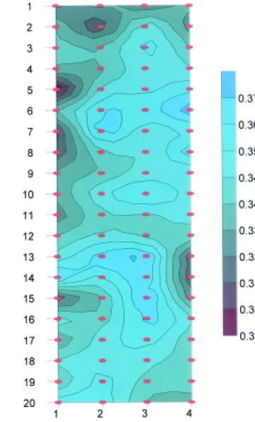
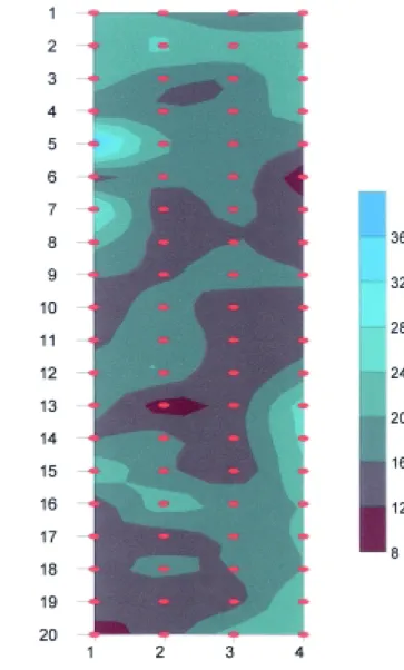
Figures 4 and 5 show soil water content isolines for the same dates and depths, calculated with the aid of the software Surfer version 5.0, Golden Software, Inc. They also show a great spatial variability, which is stable in time since the positions of the driest and wettest areas do not change significantly.
For the same dates, soil water storage of the layer
Figure 1 - Soil water content distribution for two dates 02/21/1995 and 06/07/1995 and one depth (z=0.25 m). Data are presented in a transect disposing the four lines of the grid in sequence.
Figure 3 - Histogram of the normal distribution of the soil water content at 06/07/1995 (z=0.25 m).
Figure 2 - Histogram of the normal distribution of the soil water content at 02/21/1995 (z=0.25 m).
0 to 0.75 m was calculated using the θ measurements at depths 0.25 and 0.50 m. The result is also presented in the form of a transect (Figure 6), and as isolines (Figure 7). In this case, the average value was 296 mm, the standard deviation 5.61 and the CV 1.89 %.
0.28 0.30 0.32 0.34 0.36 0.38 0.40 0 5 10 15 20 25 Fr eque ncy
Soil water content classes,θ (m3 m-3
)
0.35 0.36 0.37 0.38 0.39 0.40 0.41 0 2 4 6 8 10 F requen cy
Soil water content classes, θ m3 m-3
0.28 0.30 0.32 0.34 0.36 0.38 0.40 042
0 10 20 30 40 50 60 70 80
Depth = 0.25m
21/02/1995 07/06/1995 So il wa te r co nt en t, θ (m
3 m -3)
Figure 4 - Soil water content isolines for date (02/21/1995) at depth z=0.25 m. The points correspond to acess tube positions.
Considering the wettest set of θ (0.25 m) data (02/21/1995, Figure 1) as being the field capacity of the profile to be irrigated, irrigation water depths LL were calculated for the 80 locations, using equation (1) with the actual soil water contents θ as being those of the driest date (Figure 1). They are also presented as a transect (Figure 8) and as isolines (Figure 9). The average value is 18 mm, with a standard deviation of 5.23 mm2, and a CV of 29.3%. This high variability of LL speaks for itself in the case of decision making in relation to irrigation water depths. The lowest value is 9 mm and the largest 41mm. If irrigation is applied according to the average value of 18mm, points of the field will receive an excess of 23 mm, i.e., 128% over the average, and other points a deficit of 9 mm, i.e., 50% below average.
To establish irrigation water depths for projects of irrigation systems design, average field capacity
Figure 5 - Soil water content isolines for date (06/07/1995) at depth z=0.25 m. The points correspond to acess tube positions.
Figure 6 - Soil water storage (A) of the layer = 0 to 0.75 m for 02/21/1995.
Figure 7 - Soil water storage isolines at the layer of 0 - 0.75m for 02/21/1995. The points correspond to acess tube positions.
0 10 20 30 40 50 60 70 80
280 290 300 310 320
Depth: 0 to 0.75m
S
o
il w
a
te
r
s
tor
age,
A
(
m
m)
P oints of the transect
Figure 9 - Irrigation water depths (LL) isolines for the depth 0.25 m. The points correspond to acess tube positions.
Figure 8 - Irrigation water depths (LL) at the depth = 0.25 m, calculated for the 80 locations.
0 10 20 30 40 50 60 70 80 0
5 10 15 20 25 30 35 40 45 50
Irr
igat
ion
w
at
er
dept
hs
, LL (
m
m
)
In conclusion it might be said that due to the shown field soil water variability, the search for better values of field capacity of a given soil does not necessarily imply in better estimates of irrigation water depths, and that irrigations based on the replacement of the lost water by evapotranspiration are simpler and sufficient to meet crop demand.
REFERENCES
FALLEIROS, M.C.; SANCHEZ, A.R.; SOUZA, M.D.; BACCHI, O.O.S.; PILOTTO, J.E.; REICHARDT, K. Neutron probe measurement of soil water content close to soil surface. Scientia Agricola, v.50, p.333-337, 1993.
FRIZZONE, J.A. Irrigação por aspersão: uniformidade e eficiência. Piracicaba: USP, ESALQ, Depto. de Engenharia Rural, 1992. 53p. (Série Didática, 3)
WARRICK, A.W.; NIELSEN D.R. Spatial variability of soil physical properties in the field. In: HILLEL, D. (Ed.) Applications of soil physics. New York: Academic Press, 1980. p.319-344.