Towards a rigorous assessment of systems biology models: the DREAM3 challenges.

(1)

Towards a Rigorous Assessment of Systems Biology

Models: The DREAM3 Challenges

Robert J. Prill1, Daniel Marbach2, Julio Saez-Rodriguez3,4, Peter K. Sorger3,4, Leonidas G. Alexopoulos5, Xiaowei Xue6, Neil D. Clarke6, Gregoire Altan-Bonnet7, Gustavo Stolovitzky1*

1IBM T. J. Watson Research Center, Yorktown Heights, New York, United States of America,2Laboratory of Intelligent Systems, Ecole Polytechnique Fe´de´rale de Lausanne, Lausanne, Switzerland,3Department of Systems Biology, Harvard Medical School, Boston, Massachusetts, United States of America,4Department of Biological Engineering, Massachusetts Institute of Technology, Cambridge, Massachusetts, United States of America,5Department of Mechanical Engineering, National Technical University of Athens, Athens, Greece,6Genome Institute of Singapore, Singapore, Singapore,7Program in Computational Biology and Immunology, Memorial Sloan-Kettering Cancer Center, New York, New York, United States of America

Background: Systems biology has embraced computational modeling in response to the quantitative nature and increasing scale of contemporary data sets. The on-slaught of data is accelerating as molecular profiling technology evolves. The Dialogue for Reverse Engineering Assessments and Methods (DREAM) is a community effort to catalyze discussion about the design, application, and assess-ment of systems biology models through annual reverse-engineer-ing challenges.

Methodology and Principal Find-ings:We describe our assessments of the four challenges associated with the third DREAM conference which came to be known as the DREAM3 challenges: signaling cas-cade identification, signaling re-sponse prediction, gene expression prediction, and the DREAM3 in silico network challenge. The chal-lenges, based on anonymized data sets, tested participants in network inference and prediction of mea-surements. Forty teams submitted 413 predicted networks and mea-surement test sets. Overall, a hand-ful of best-performer teams were identified, while a majority of teams made predictions that were equivalent to random. Counterin-tuitively, combining the predictions of multiple teams (including the weaker teams) can in some cases improve predictive power beyond that of any single method.

Conclusions: DREAM provides valuable feedback to practitioners of systems biology modeling. Les-sons learned from the predictions of the community provide much-needed context for interpreting claims of efficacy of algorithms described in the scientific literature.

Introduction

Computational models of intracellular networks are a mainstay of systems biology. Researchers have used a variety of algorithms to deduce the structure of very different biological and artificial networks [1] and have evaluated their success using various metrics [2–8]. What is needed is a fair comparison of the strengths and weaknesses of the methods and a clear sense of the reliability of the network models they produce.

The Dialogue on Reverse Engineering Assessment and Methods (DREAM) pro-ject ‘‘takes the pulse’’ of the current state of the art in systems biology modeling [9,10]. DREAM is organized around annual reverse-engineering challenges whereby teams download data sets from recent unpublished research, then attempt to recapitulate some withheld details of the data set. A challenge typically entails inferring the connectivity of the molecular networks underlying the measurements, predicting withheld measurements, or related reverse-engineering tasks. Assess-ments of the predictions are blind to the methods and identities of the participants. The format of DREAM was inspired by the Critical Assessment of techniques for protein Structure Prediction (CASP) [11]

whereby teams attempt to infer the three-dimensional structure of a protein that has recently been determined by X-ray crystal-lography but temporarily withheld from publication for the purpose of creating a challenge. Instead of protein structure prediction, DREAM is focused on network inference and related topics that are central to systems biology research. While no single test of an algorithm is a panacea for determining efficacy, we assert that the DREAM project fills a deep void in the validation of systems biology algorithms and models. The assessment provides valuable feedback for algorithm designers who can be lulled into a false sense of security based on their own internal benchmarks. Ulti-mately, DREAM and similar initiatives may demystify this important but opaque area of systems biology research so that the greater biological research community can have confidence in this work and build new experimental lines of research upon the inferences of algorithms.

Evolution of the DREAM Challenges At the conclusion of the second DREAM conference [10], a few voices of reason suggested that reverse-engineering chal-lenges should not be solely focused on the network inference. As the argument goes, only that which can be measured should be

Citation:Prill RJ, Marbach D, Saez-Rodriguez J, Sorger PK, Alexopoulos LG, et al. (2010) Towards a Rigorous Assessment of Systems Biology Models: The DREAM3 Challenges. PLoS ONE 5(2): e9202. doi:10.1371/ journal.pone.0009202

Editor:Mark Isalan, Center for Genomic Regulation, Spain

ReceivedNovember 19, 2009;AcceptedJanuary 19, 2010;PublishedFebruary 23, 2010

Copyright: ß2010 Prill et al. This is an open-access article distributed under the terms of the Creative Commons Attribution License, which permits unrestricted use, distribution, and reproduction in any medium, provided the original author and source are credited.

Funding:G.S. and R.P. acknowledge support of the National Institutes of Health (NIH) Roadmap Initiative, the Columbia University Center for Multiscale Analysis Genomic and Cellular Networks (MAGNet), and the IBM Computational Biology Center. L.A. acknowledges funding from the Marie Curie MIRG-CT-2007-46531 grant. J.R. acknowledges funding from NIH P50-GM68762 and U54-CA11296 grants. G.A.-B. acknowledges funding from a National Science Foundation (NSF) grant 0848030 and NIH grant AI083408. The funders had no role in study design, data collection and analysis, decision to publish, or preparation of the manuscript.

Competing Interests:The authors have declared that no competing interests exist.

(2)

predicted. Since knowledge of biological networks is actually a model in its own right, it may be counterproductive to evaluate networks for which no ground truth is known. We agree that the positivist viewpoint has merit both as a matter of philosophy and practicality. Some of the DREAM3 challenges reflect this attitude, which was a shift from previous challenges which were squarely focused on network inference.

Nevertheless, the systems biology com-munity continues to assert—through fund-ing opportunities, conference attendance, and the volume of publications—that network inference is a worthwhile scien-tific endeavor. Therefore, DREAM con-tinues to provide a venue for vetting algorithms that are claimed to reverse-engineer networks from measurements. Despite the above mentioned criticisms, network inference challenges are a main-stay of DREAM. To contend with the criticism that no ground truth is known for molecular networks, the organizers must occasionally tradeoff realism for truth— generating in silico(i.e., simulated) data is one way that this problem is mitigated.

We describe the results of the DREAM3 challenges: signaling cascade identifica-tion, signaling response predicidentifica-tion, gene expression prediction, andin siliconetwork inference. The fourth challenge was sim-ilar to the DREAM2 in silico network inference challenge [10] which enabled a cursory analysis of progress (or lack thereof) in the state of the art of network inference. The best-performer strategies in each challenge are described in detail in accompanying publications in this PLoS ONE Collection. Here, our focus is the characterization of the efficacy of the reverse-engineering community as a whole. The results are mixed: a handful of best-performer teams were identified, yet the performance of most teams was not all that different from random.

In the remainder of the Introduction we describe each of the four DREAM3 challenges. In Results and Discussion, we summarize the results of the prediction efforts of the community, identify best-performer teams, and analyze the impact of the community as a whole. Readers interested in a particular challenge can read the corresponding sub-sections with-out loss of continuity. Finally, we present the conclusions of this community-wide experiment in systems biology modeling.

The DREAM3 Challenges

In this section we describe the challeng-es as they were prchalleng-esented to the

partici-pants. Additionally, we elaborate on the experimental methods at a level of detail that was not provided to the participants. We then go on to describe the basis of the assessments—‘‘gold standard’’ test sets, scoring metrics, null models andp-values. The complete challenge descriptions and data are archived on the DREAM website [12].

Signaling Cascade Identification The signaling cascade identification challenge explored the extent to which signaling proteins are identifiable from flow cytometry data. Gregoire Altan-Bonnet of Memorial Sloan-Kettering Can-cer Center generously donated the data set consisting of pairwise measurements of proteins that compose a signaling pathway in T cells [13]. The data producer, cell type, and protein identities were not disclosed to participants until the results of the challenge were released.

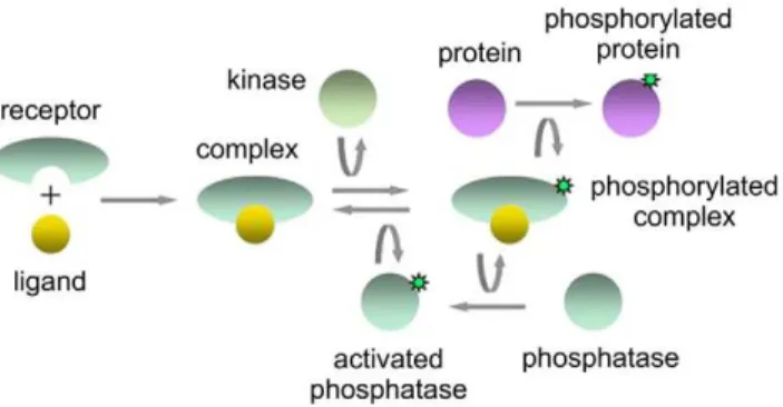
Protein concentrations in a signaling network were measured in single cells by antibody staining and flow cytometry. Participants were provided a network diagram (Figure 1) and pairwise measure-ments of four signaling proteins (denoted x1, x2, x3, x4) obtained from single cells. The pairs of proteins (x1, x4), (x2, x4), and (x3, x4) were simultaneously measured in separate assays. The task was to identify each of the measured proteins (x1, x2, x3, x4) from among the seven molecular species (complex, phosphorylated com-plex, protein, phosphorylated protein, kinase, phosphatase, and activated phosphatase).

The experimental setup allowed for external control over the signaling network through the ligand that binds to the membrane-bound receptor. Two types of ligands, weak and strong (i.e., with differ-ent potency), in differdiffer-ent concdiffer-entrations,

were used. Five concentrations of strong ligand (including none) and seven concen-trations of weak ligand (including none) were applied to approximately104_{cells in} separate experiments. In total, data from 36 experiments corresponding to the various combinations of quantified pro-teins, ligand type, and ligand concentra-tion were provided. The biological moti-vation of the T cell experiment is discussed in [13].

Basis of assessment. Participants were instructed to identify each of each of the four measured proteins (x1, x2, x3, x4) as a molecular species (kinase, phosphatase, etc.). Each measurement could only be identified as a single molecular species, and each molecular species could be assigned to at most one measurement. For example, if measurement x1 was identified as the kinase then no other measurement could also be identified as the kinase. Submissions were scored by the probability that a random assignment table would result in as many correct identifications as achieved by the participant.

There are 840 possible assignment tables for seven molecular species and four measurements (i.e., 7|6|5|4). The probability of guessing the gold standard assignment table by chance is 1/840, which we denotea. By enumerat-ing the 840 tables and countenumerat-ing the number of correct (or incorrect) assign-ments in each table, we obtain the probability of correctly identifying four, three, two, one, or zero molecular species. It can be shown that the probability P(:) of making some number of correct identifi-cations is exactly

P(4 correct)~ 1

7|6|5|4~a

Figure 1. The objective of the signaling cascade identification challenge was to identify some of the molecular species in this diagram from single-cell flow cytometry measurements. The upstream binding of a ligand to a receptor and the downstream phosphorylation of a protein are illustrated.

(3)

P(3 correct)~ 4

1

1 7|6|5|

3 4~12a

P(2 correct)~

4

2

!

1 7|6

1 5z

3 5|

3 4

~₇₈a

P(1 correct)~

4

3

!

1 7

2 6

1 5z

4 5|

3 4

z3

6 1 5z

3 5|

3 4

~284a

P(0correct)~3

7 2 6

1 5z

4 5|

3 4

z4

6 1 5z

3 5|

3 4

z3

7 2 6

1 5z

4 5|

3 4

z3

6 1 5z

3 5|

3 4

~465a:

In addition to assigning a score to each team, we characterized the efficacy of the community as a whole. For example, what is the probability that five teams would correctly identify the same protein? To compute p-values for community-wide outcomes such as this we used the binomial distribution which is explained in Results.

Signaling Response Prediction The signaling response prediction chal-lenge explored the extent to which the responses to perturbations of a signaling pathway can be predicted from a set of training data consisting of perturbations (environmental cues and signaling protein inhibitors) and their responses. Peter Sorger of Harvard Medical School gener-ously donated the data for this challenge consisting of time-series measurements of a signaling network measured in human hepatocytes [14,15]. The task entailed predicting some phosphoprotein and cy-tokine measurements that were withheld from the participants.

Approximately 10,000 fluorescence mea-surements proportional to the concentration of intracellular phosphorylated proteins and extracellular cytokines were acquired in normal human hepatocytes and the hepa-tocellular carcinoma cell line HepG2 using the using the Luminex (Austin, TX) 200

xMAP system. The data set consisted of measurements of 17 phosphoproteins at 0 minutes, 30 minutes, and 3 hrs following stimulation/perturbation of the two cell types. Additionally, 20 cytokines were quan-tified at 0 minutes, 3 hours, and 24 hours following stimulation/perturbation of the two cell types. Data were processed and visualized using the open-access MATLAB-based software, DataRail [16]. The cell types and protein identities were disclosed so that participants could draw upon the existing signal transduction literature.

In each experiment, a combination of a single chemical stimulus and a single chemical perturbation to the signaling network were simultaneously applied, and measurements of either the signaling network proteins or cytokines were taken (Figure 2A). Seven stimuli were investigat-ed: INFc, TNFa, IL1a, IL6, IGF-I, TGFa, and LPS (Table 1). Also, seven chemical inhibitors of specific signaling proteins were investigated, which selectively inhib-ited the activities of MEK12, p38, PI3K, IKK, mTOR, GSK3, or JNK. All pairs of stimulus/inhibitor combinations (a total of 64) were applied to both cell types and measurements of fluorescence for individ-ual proteins or cytokines were taken at the indicated time points. Fluorescence was reported in arbitrary units from 0 to *29000. The upper limit corresponded to saturation of the detector. Signal

intensity below 300 was considered noise. Fluorescence intensity was approximately linear with concentration in the mid-dynamic range of the detector.

The challenge was organized in two parts that were evaluated separately: the phosphoprotein subchallenge and the cy-tokine subchallenge. The complete data set (training and test) in the signaling response prediction challenge was com-posed of fluorescence measurements of phosphoproteins and cytokines in cells exposed to pairwise combinations of eight stimuli and eight signaling-network-pro-tein inhibitors, for a total of 64 stimulus/ inhibitor combinations (including zero concentrations). Fifty-seven of the combi-nations composed the training set, and seven combinations composed the test set. The phosphoprotein subchallenge solicited predictions for 17 phosphoproteins, in two cell types (normal, carcinoma), at two time points, under seven combinatoric stimu-lus/inhibitor perturbations for a total of 476 predictions. Likewise, the cytokine subchallenge solicited predictions for 20 cytokines for a total of 560 predictions. The biological motivation for the hepato-cyte experiment is described in [14,15].

Basis of assessment. Assessment of the predicted measurements was based on a single metric, the normalized squared error over the set of predictions in each subchallenge,

Figure 2. The objective of the signaling response prediction challenge was to predict the concentrations of phosphoproteins and cytokines in response to combinatorial perturbations the environmental cues (stimuli) and perturbations of the signaling network (inhibtors).(a) A compendium of phosphoprotein and cytokine measurements was provided as a training set. (b) Histograms (log scale) of the scoring metric (normalized squared error) for 100,000 random predictions were approximately Gaussian (fitted blue points). Significance of the predictions of the teams (black points) was assessed with respect to the empirical probability densities embodied by these histograms. Scores of the best-performer teams are denoted with arrows.

(4)

Norm:Sq:Error~X n

i~1

(^xxi{xi)2

s2_Techzs2_Bio

, ð1Þ

wherexiis theith measurement,^xxiis theith prediction, s2_Tech is the technical variance, and s2_Bio is the biological variance. The variances were parametrized as follows: sTech= 300 (minimum sensitivity of the detector for antibody-based detection assays) and sBio= 0.8|xi (product of the coefficient of variation and the measurement). Note that the squared prediction error is normalized by an estimate of the measurement variance, a sum of the biological variance and the technical variance. A probability distri-bution for this metric was estimated by simulation of a null model.

The null model was based on a naive approach to solving the challenge. Essen-tially, participants were provided a spread-sheet of measurements with some entries

missing. The columns of the spreadsheet corresponded to the phosphoproteins or cytokines (depending on the subchallenge); rows corresponded to various perturba-tions of stimuli and inhibitors. We ran-domly ‘‘filled-in’’ the spreadsheet by choosing values for the missing entries, with replacement, from the corresponding column. Since each protein or cytokine had a characteristic dynamic range, this procedure ensured that the random pre-dictions were drawn from the appropriate order of magnitude of fluorescence. This procedure was performed 100,000 times. Parametric curves were fit to the histo-grams (Figure 2B) to extrapolate the probability density beyond the range of the histogram (i.e., to computep-values for teams that did far better or worse than this null model). The procedure for curve-fitting was described previously [10]. Briefly, an approximation of the empirical probability density was given by stretched

exponentials with different parameters to the right and left of the mode of the distribution, with functional form

pdf(x)~hmaxexp½

{bw(x{xmax)cwforx§xmax

hmaxexp½{bv(x{xmax)cvforxvxmax

,ð2Þ

wherehmax is the maximum height of the histogram, xmax is the position of hmax, and bw, bv, cw, and cv are fitted parameters.

Gene Expression Prediction

The gene expression prediction chal-lenge explored the extent to which time-dependent gene expression measurements can be predicted in a mutant strain of S. cerevisiae (budding yeast) given complete expression data for the wild type strain and two related mutant strains. Experi-mental perturbations involving histidine biosynthesis provided a context for the challenge. Neil Clarke of the Genome Institute of Singapore generously donated unpublished gene expression measure-ments for this challenge.

The yeast transcription factors GAT1, GCN4, and LEU3 regulate genes involved in nitrogen and/or amino acid metabolism. They were disrupted in three mutant strains denotedgat1D,gcn4D, andleu3D. These genes are considered nonessential since the deletion strains are viable. Ex-pression levels were assayed separately in the three mutant strains and in the wild type strain at times 0, 10, 20, 30, 45, 60, 90 and 120 minutes following the addition of 3-aminotriazole (3AT) as described [17]. 3AT inhibits an enzyme in the histidine biosynthesis pathway and, in the appropri-ate media (used in these experiments), has the effect of starving the cells for this essential amino acid.

Expression measurements were ob-tained using DNA microarrays (Affymetrix YGS98 GeneChip). Two biological repli-cates (i.e., independent cultures) and an additional technical replicate (i.e., inde-pendent labeling and hybridization of the same culture) were performed. Measure-ments were normalized using the RMA algorithm [18] within the commercial software package, GeneSpring. Values were median normalized within arrays prior to the calculation of fold-change. The mean hybridization value for each probe set was obtained from the three replicates and was normalized to the mean value for the probe set in the wild-type samples at time zero. Values were provid-ed as the log (base two) of the ratio of the indicated experimental condition (i.e., strain and time point) relative to the wild type strain at time zero.

(2)

Table 1.The signaling response prediction challenge solicited predictions of the concentrations of 17 phosphoproteins and 20 cytokines.

Phosphoproteins (17) Inhibitors (7) Cytokines (20) Stimuli (7)

Akt IL1b

ERK1/2 IL4

GSK-3alpha/beta IL6 IL6

IkappaB-alpha IL8

JNK JNK-i IL10

p38 MAPK p38-i IL15

p70 S6 kinase GCSF

p90RSK GMCSF

STAT3 IP10

c-Jun MCP1

CREB MIP1a

Histone H3 MIP1b

HSP27 PDGFbb

IRS-1 RANTES

MEK1 VEGF

p53 GROa

STAT6 ICAM1

MEK12-i MIF

PI3K-i MIG

IKK-i SDF1a

mTOR-i INFg

GSK3-i TNFa

IL1a

IGF-I

TGFa

LPS

The data set underlying this challenge consisted of phosphoprotein and cytokine concentrations in response to 49 combinatoric perturbations of seven protein-specific inhibitors and seven stimuli.

(5)

The fifty genes composing the test set were selected by subjective criteria, but with an eye towards enriching for genes that are significantly regulated in at least one strain, or are bound by one or more of the transcription factors according to ChIP-chip data, or are relatively strongly predicted to be bound based on a PWM-based promoter occupancy calculation [19]. Thus, the expression profiles for these genes tend to be somewhat more explicable than would be the case for randomly selected genes. Nevertheless, it was trivial to find genes for which an explanation for the expression profiles was not obvious, and there are many such genes among the fifty prediction targets.

A quantitative prediction of gene ex-pression changes is far beyond state of the art at this time, so participants were asked to predict the relative expression levels for 50 genes at the eight time points in the gat1D strain. Participants were provided complete expression data for the other strains, as well measurements for the genes that were not part of the set of 50 challenge genes ingat1D. Predictions for each time point were submitted as a ranked list with values from 1 to 50 sorted from most induced to most repressed compared to the wild type expression at time zero.

Basis of assessment. Participants submitted a spreadsheet of 50 rows (genes) by eight columns (time points). Submissions were scored using Spearman’s rank correlation coefficient between the predicted and measured gene expression at each of the eight time points. The same statistic was also computed with respect to each gene across all time points. Thus, we evaluated predictions using two different tests of similarity to the gold standard which we call the time-profiles and gene-profiles, respectively.

For each column of the predicted matrix of relative expression, we obtained a correlation coefficient and its correspond-ingp-value under the null hypothesis that the ranks are randomly distributed. From the columnp-values we arrived at a single summaryp-value for all eight time points using the geometric mean of individualp -values (i.e., (p1p2p3p4p5p6p7p8)1=8). The same procedure was performed on the row p-values to arrive at a summaryp-value for the 50 genes. Finally, the score used to assess best-performers was computed from the two summaryp-values

score~{1

2log10(pT|pG), ð3Þ

wherepTis the overallp-value for the

time-profiles (columns) andpG is the overallp -value for the gene-profiles (rows). The higher the score, the more significant the prediction.

In SilicoNetwork Inference

Thein siliconetwork inference challenge explored the extent to which gene net-works of various sizes and connection densities can be inferred from simulated data. Daniel Marbach of Ecole Polytech-nique Fe´de´rale de Lausanne extracted the challenge networks as subgraphs of the currently accepted E. coli and S. cerevisiae gene regulation networks [8] and imbued the networks with dynamics using a thermodynamic model of gene expression. Thein silico‘‘measurements’’ were gener-ated by continuous differential equations which were deemed reasonable approxi-mations of gene expression regulatory functions. To these values was added a small amount of Gaussian noise to simu-late measurement error.

The simulated data was meant to mimic three typical types of experiments: (1) time courses of a wild type strain following an environmental perturbation (i.e., trajecto-ries); (2) knock-down of a gene by deletion of one copy in a diploid organism (i.e., heterozygous mutants); (3) knock-out of a gene by deletion of both copies in a diploid organism (i.e., homozygous null mutants). Technically, a haploid organism such asE. coli can not be a heterozygote, but since this data only existsin silicowe did not see harm in the use of this term. A trajectory of the wild-type response to an environ-mental perturbation was simulated by a random initialization of the simulation. A heterozygous knock-down mutant was simulated by halving the wild type con-centration of the gene. A homozygous knock-out mutant was simulated by floor-ing the wild type concentration of the gene to zero.

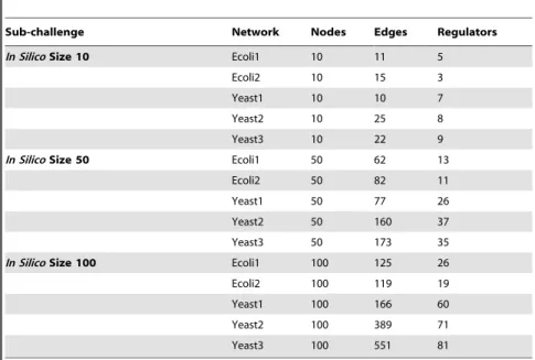
The challenge was organized into three parts: the 10-node subchallenge, the 50-node subchallenge, and the 100-50-node subchallenge. Within each sub-challenge, participants were required to predict five networks, denoted Ecoli1, Ecoli2, Yeast1, Yeast2, Yeast3. Completion of a subchal-lenge required submission of predictions for all five of the networks in the subchallenge. Participants were encour-aged, but not required, to perform all three subchallenges on networks of various sizes. Some of the gross topological properties of the fifteen gold standard networks are illustrated in Table 2.

Complete steady state expression infor-mation was provided for the wild type and mutant strains. In other words, in the

10-node subchallenge, all ten genes were knocked-down and knocked-out, one at a time, while the remaining nine measure-ments were provided. Various numbers of trajectories from random initializations were provided depending on the subchal-lenge. Four, 23, and 46 trajectories were provided for the 10-node, 50-node, and 100-node subchallenges, respectively.

Participants were asked to predict the directed, unsigned networks from in silico gene expression data sets. A network prediction was submitted in the form of a ranked list of potential network edges ordered from most reliable to least reli-able. In other words, the edges at the top of the list were believed to be present in the network and the edges at the bottom of the list were believed to be absent from the network. This submission format was chosen because it does not require the researcher to impose a particular threshold for calling an edge present or absent. Also, it can be scored without imposition of a specific threshold. An example of the file format of a network prediction is illustrat-ed in Table 3.

Basis of assessment. From the ranked edge-list (Table 3), a particular concrete network withkedges is obtained by designating the first k edges present and the remaining edges absent. Then,k is a parameter that controls the number of edges in a predicted network. Various performance metrics were computed ask was varied from 1 toT, the total number of possible directed edges, where T~N(N{1) and N is the number of nodes in the network.

Two parametric curves, the precision-recall (P-R) curve and the the receiver operating characteristic (ROC) curve, were traced by scanning k~1,. . .,T. Recallis a measure of completeness,

rec(k)~TP(k)

P ,

where TP(k) is the number of true positives at threshold k, and P is the number of positives (i.e., gold standard edges).Precisionis a measure of fidelity,

prec(k)~ TP(k)

TP(k)zFP(k)~ TP(k)

k ,

(6)

(AUPR) is a single number that summa-rizes the precision-recall tradeoff. Similar-ly, the receiver operating characteristic (ROC) curve graphically explores the tradeoff between the true positive rate (TPR) and the false positive rate (FPR). TPR(k) is the fraction of positives that are correctly predicted at thresholdk,

TPR(k)~TP(k)

P :

(Note that TPR is equivalent to recall.) FPR(k) is the fraction of negatives that are

incorrectly predicted at thresholdk,

FPR(k)~FP(k)

N :

Negativedenotes the absence of an edge in the gold standard network. The area under the ROC curve (AUROC, also denoted AUC in the literature) is a single number that summarizes the tradeoff between TPR(k) and FPR(k) as the parameter k is varied. Using both the AUPR and the AUROC metrics, we gain a fuller characterization of the prediction

than using either alone. For example, the P-R curve indicates whether the first few edge predictions at the top of the predic-tion list are correct. The ROC curve does not provide this information.

A technical point is the issue of how to score a truncated prediction list, where fewer than the total number of possible edges are submitted. A methodology is in place from the previous DREAM assess-ment [10]. If a prediction list does not contain a complete ordering of all possible N(N{1)edges, we ‘‘add’’ the missing edges in random order at the end of the list. The addition takes place in an analytical way.

A team’s score for a subchallenge depended on quite a few calculations. Each of the five network predictions (Ecoli1, Ecoli2, Yeast1, Yeast2, Yeast3) were evaluated by AUPR and AUROC. P-values for these assessments were ob-tained from the empirical distributions described above. The five AUPRp-values were condensed to an overall AUPR p -value using the geometric mean of indi-vidualp-values (i.e.,(p1p2p3p4p5)1=5). The same procedure was performed on the five AUROC p-values to arrive at an overall AUROCp-value. Finally, the score for the team was computed as

score~{1

2log10(pAUPR|pAUROC), ð4Þ

where pAUPR and pAUROC are the overall p-values for AUPR and AUROC, respec-tively. The higher the score, the more significant the network prediction.

Results and Discussion

The DREAM3 challenges were posted on the DREAM website on June 15, 2008. Submissions in response to the challenges were accepted on September 15, 2008. Forty teams submitted 413 predicted networks and test set predictions in the various challenges. The anonymous results were posted on the DREAM website [12] on October 15, 2008.

In this section, we describe our assess-ment of the predictions supplied by the community. Our dual goals are to identify the best-performers in each challenge and to characterize the efficacy of the commu-nity as a whole. We highlight the best-performer strategies and comment on some of the sub-optimal strategies. Where possible, we attempt to leverage the community intelligence by combining the predictions of multiple teams into a consensus prediction.

Best-performers in each challenge were identified by statistical significance with respect to a null model combined with a Table 2.Statistical properties of the gold standard networks in thein siliconetwork

inference challenge.

Sub-challenge Network Nodes Edges Regulators

In SilicoSize 10 Ecoli1 10 11 5

Ecoli2 10 15 3

Yeast1 10 10 7

Yeast2 10 25 8

Yeast3 10 22 9

Ecoli2 50 82 11

Yeast1 50 77 26

Yeast2 50 160 37

Yeast3 50 173 35

Ecoli2 100 119 19

Yeast1 100 166 60

Yeast2 100 389 71

Yeast3 100 551 81

In each of the three sub-challenges the number of nodes was held constant but the number of edges and regulator nodes was not. There were five gold standard networks in each of the three sub-challenges (which were treated as three separate contests).

doi:10.1371/journal.pone.0009202.t002

Table 3.Format of a predicted network in thein siliconetwork inference challenge.

Source Node Target Node Confidence Scoring Cutoff (k)

G85 G1 1.00 1

G85 G10 0.99 2

G10 G85 0.73 3

G99 G52 0.44 4

.. .

G10 G3 0.01 N(N-1)

Predicted edges were to be ranked from most confidence to least confidence that the edge is present in the network. A directed edge is denoted by a source and target node and an arbitrary (non-increasing) score between one (most confidence) to zero (least confidence). Thus, edges that are predicted to exist in the network should be at the top of the list and those predicted not to exist in the network should be at the bottom of the list. To evaluate the predicted network, two metrics—area under the ROC curve and area under the precision-recall curve—were computed by scanning all possible decision boundaries (i.e., k = 1, k = 2, etc.) up to the maximum number of possible directed edges (excluding self-edges).

(7)

clear delineation from the rest of the participating teams (e.g., an order of magnitude lower p-value compared to the next best team). Occasionally, this criterion identified multiple best-perform-ers in a challenge.

Signaling Cascade Identification Seven teams submitted predictions for the signaling cascade identification chal-lenge as described in the Introduction. Submissions were scored based on the probability that a random solution to the challenge would achieve at least as many correct protein identifications as the sub-mitted solution.

Five of seven teams identified two of the four proteins correctly (though not the same pair) (Table 4). One team identified only one protein correctly and one team did not identify any correctly. Thep-value for a team identifying two or more proteins correctly is 0.11, as described in the Introduction. On the basis of this p -value, this challenge did not have a best-performer. However, in the days following the conference, follow-up questions from some of the participants to the data provider revealed a misrepresentation in how the challenge was posed, which probably negatively impacted the teams’ performances. The source of the confusion is describe below.

Despite that no individual team gained much traction in solving this challenge, the community as a whole seemed to possess intelligence. For example, five of seven teams correctly identified two proteins (though not the same pair). While such a performance is not significant on an individual basis, the event of five teams correctly identifying two proteins is un-likely to occur by chance. Under the

binomial distribution, assuming indepen-dent teams, the probability of five or more teams correctly identify two or more proteins is2:6|10{4_.

Summing over the predictions of all the teams we obtain Figure 3. For example, five of seven teams correctly identified x1 as the kinase. The probability that five or more teams would pick the same table entry is 9:7|10{4_{. Similarly, the} proba-bility of three or more teams identifying the same pair of proteins (e.g., kinase, phosphoprotein) is4:4|10{4_.

The assumption of independence is implicit in the null hypothesis underlying these p-values. Rejection of the null hypothesis on the basis of a smallp-value indicates that there is a correlation be-tween the teams. This correlation can be interpreted as a shared success within the community. In other words, the commu-nity exhibits some intelligence not evi-denced in the predictions of the individual teams. Based on this assessment of the community as a whole, we conclude that some structural features of the signaling cascade were indeed identified from flow cytometry data.

The community assessment suggests that a mixture of methods may be an advantageous strategy for identifying sig-naling proteins from flow-cytometry data. A simple strategy for generating a consen-sus prediction is illustrated by Figure 3 in which the total number of predictions made by the community for each possible assignment are indicated along with the corresponding p-values indicating the probability of such a concentration of predictions in a single table entry. The the kinase and phosphorylated protein are the only identifications (individually) sig-nificant at pv₀:₀₅. This analysis also reveals clustering of incorrect predic-tions—the phosphatase was most often confused with the activated phosphatase, and the phosphorylated protein was most often confused with the phosphorylated ligand-receptor complex—but these mis-identifications were not significant.

Mea culpa: a poorly posed challenge.

There are three conjugate pairs of species in the signaling pathway: complex/phospho-complex, protein/phosho-protein, and phosphatase/activated phosphatase. The challenge description led participants to believe that each measured species (x1,…, x4) may match one of the six individ-ual species. In fact, measurement x3 corresponded to total protein (inactive and active forms). Likewise, measurement x2 corresponded to total phosphatase (inactive and active forms). It would be highly unusual for an antibody to target one

epitope of a protein to the exclusion of a phosphorylated epitope. That is, it would be difficult but not impossible to raise an antibody that reacted with only the unphosphorylated version of a protein. This serious flaw in the design of the challenge did not come to light until after the scoring was complete.

The simultaneous identification of the upstream kinase and the downstream phosphorylated protein (Figure 3) can be explained in light of the confusion sur-rounding precisely what the measurements entailed. The measurements correspond-ing to the kinase and phosphoprotein were accurately portrayed in the challenge description whereas the total protein and total phosphatase were not.

Signaling Response Prediction Four teams participated in the signaling response prediction challenge. The phos-phoprotein subchallenge received three submissions, as did the cytokine subchal-lenge. As described in the Introduction, the task was to predict measurements of proteins and/or cytokines, in normal and cancerous cells, for combinatoric pertur-bations of stimuli and inhibitors of a signaling pathway. Submissions were scored by a metric based on the sum of the squared prediction errors (Figure 2B). In the phosphoprotein subchallenge two teams achieved a p-value orders of mag-nitude lower than the remaining other submission (Table 5). In the cytokine subchallenge one team had a substantially smaller total prediction error than the next best team. On this basis, the best-perform-ers were:

N

Genome Singapore (phosphoprotein and cytokine subchallenges): Guil-laume Bourque and Neil Clarke of the Genome Institute of Singapore, Singapore

N

Vital SIB (phosphoprotein subchal-lenge): Nicolas Guex, Eugenia Miglia-vacca, and Ioannis Xenarios of the Swiss Institute of Bionformatics, Switzerland

There are two main types of strategies that could have been employed in this challenge: to explicitly model the underly-ing signalunderly-ing network, or to model the data statistically. Both of the best-performers took a statistical approach. Vital SIB approached it as a missing data problem and used multiple imputation to predict the missing data. This involved learning model parameters by cross-validation, followed by prediction of the missing data [20]. Genome Singapore identified the Table 4.Results of the signaling

cascade identification challenge.

No. Correct

Team Identifications p-value

Team 315 2 0.11

Team 283 2 0.11

Team 106 2 0.11

Team 281 2 0.11

Team 181 2 0.11

Team 110 1 0.45

Team 286 0 1.00

Two correct identifications is not a significant performance so no team was named the best-performer.

(8)

nearest-neighbors of missing ments based on similarity of the measure-ment profiles [21]. To predict the mea-surements for an unobserved stimulus or inhibitor, they took into consideration the values observed for the nearest neighbor. Neither team utilized external data sourc-es, nor did they evoke the concept of a biological signaling network.

Surprisingly, one team in the cytokine subchallenge had a significantly larger total error than random. We investigated this strange outcome further. This team systematically under-predicted the medi-um and large intensity measurements (data not shown). This kind of systematic error was heavily penalized by the scoring metric. Nevertheless, the best-performer would have remained the same had linear correlation been used as the metric. Due to the low participation level from the community, we did not perform a com-munity-wide analysis.

Gene Expression Prediction

Nine teams participated in the gene expression prediction challenge as de-scribed in the Introduction. The task was to predict the expression of 50 genes in the gat1D strain of S. cerevisiae at eight time points. Participants submitted a spread-sheet of 50 rows (genes) by eight columns (time points). At each time point, the participant ranked the genes from most induced to most repressed compared to the wild type values at time zero.

Predic-tions were assessed by Spearman’s corre-lation coefficient and its correspondingp -value under the null hypothesis that the ranks are uniformly distributed.

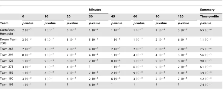
The p-values (based on Spearman correlation coefficient) computed over the set of 50 test genes at each of the eight time-points are reported in Table 6. Some trends are readily identifiable. Across the community, the least significant predic-tions were those at time zero. Relatively more significant predictions were made at 10, 20, 45, and 60 minutes, and compar-atively less significant predictions were made at 30 and 90 minutes. This analysis identified the teams that predicted well (over the 50 test genes) at each time point. We computed a summary statistic for each team using the geometric mean of the eight p-values for the individual time points.

In the above analysis, each of the eight time points was analyzed as a 50-dimen-sional vector. An alternative viewpoint is to consider each of the 50 genes as an eight-dimensional vector. We also per-formed this analysis using Spearman’s correlation coefficient computed for each gene. We computed a summary statistic for each team using the geometric mean of the 50 p-values for the individual genes (not shown). Correlation coefficients and p-values for the gene-profiles are published on the DREAM website [12].

Summary statistics from the time-profile analysis and the gene-profile analysis are

reported in Table 7. Weaker significance of gene-profilep-values compared to time-profilep-values may be due to the fact that the former are eight-dimensional vectors while the latter are 50-dimensional vec-tors. Best-performers were identified by an overall score based on the time-profile and gene-profile summary p-values. A differ-ence of one in the overall score corre-sponds to an order of magnitude differ-ence in thep-value. Two teams performed more than an order of magnitude better than the nearest competitor atpv0:05.

N

Gustafsson-Hornquist : Mika Gustafs-son and Michael Hornquist of Linko¨p-ing University, Sweden

N

Dream Team 2008 : Jianhua Ruan of the University of Texas at San Anto-nio, USA

We used hierarchically clustered heat maps to visualize the teams’ predictions (gene ranks from 1 to 50) relative to the gold standard (Figure 4A). The two best-performers were more similar to each other than either was to the gold standard. The Spearman correlation coefficient be-tween Gustafsson-Hornquist and Dream Team 2008 is 0.96, while the correlation between either team and the Gold Stan-dard is 0.67. One could reasonably presume that substantially similar methods were employed by both teams. That turns out not the be the case.

Team Gustafsson-Hornquist used a weighted least squares approach in which the prediction for each gene was a weighted sum of the values of the other genes [22]. The particular linear model they employed is called an elastic net, which is a hybrid of the lasso and ridge regression [23]. They incorporated additional data into their model, taking advantage of public yeast expression profiles and ChIP-chip data. The additional expression profiles provided more training examples from which to estimate pairwise correlations between genes. The physical binding data (ChIP-chip) was integrated into the linear model by weighting each gene’s contribution to a

Figure 3. Overlay of the assignment tables from the seven teams in the signaling cascade identification challenge.The number of teams making each assignment and thep-value is indicated. Thep-value expresses the probability of a such a concentration of random guesses in the same table entry. Highlighted entries are correct. Five teams correctly identified species x1 as the kinase, a significant event for the community despite that no team had a significant individual performance.

doi:10.1371/journal.pone.0009202.g003

Table 5.Results of the signaling response prediction challenge.

Subchallenge Team Norm. Sq. Error p-value

Phosphoprotein Vital SIB 3102 210{22

GenomeSingapore 3310 410{22

Team 302 11329 710{14

Cytokine GenomeSingapore 4462 810{36

Team 302 13995 410{9

Team 126 29795 1

(9)

prediction based on the number of com-mon transcription factors the pair of genes shared.

Dream Team 2008 did not use any additional data beyond what was provided in the challenge. Rather, they employed a k-nearest neighbor (KNN) approach to predict the expression of a gene based on the expression of other genes in the same strain at the same time point [24]. The Euclidean distance between all pairs of genes was determined from the strains for which complete expression profiles were provided. The predicted value of a gene was the mean expression of thek -nearest-neighbors. The parameter k was chosen by cross-validation; k~10 was used for prediction.

Does the community possess an intelli-gence that trumps the efforts of any single

team? To answer this question we created a consensus prediction by summing the predictions of multiple teams, then re-ranking. The results of this analysis are shown in Figure 4B which traces the overall score of the consensus prediction as lower-significance teams are included. The first consensus prediction includes the best and second-best teams. The next consensus prediction includes the top three teams, and so on.

The consensus prediction of the top four teams had a higher score than the best-performer, which is counter-intuitive since the third and fourth place teams individ-ually scored much lower than the best-performer (Figure 4B). Furthermore, the inclusion of all teams in the consensus prediction scored about the same as the best-performer. This result suggests that,

given the output of a collection of algorithms, combining multiple result sets into a consensus prediction is an effective strategy for improving the results.

We assigned a difficulty level to each gene based on the accuracy of the community. For each gene, we computed the geometric mean of the gene-profilep -values over the nine teams, which we interpreted as the difficulty level of each gene. The five best-predicted genes were: arg4, ggc1, tmt1, arg1, and arg3. The five worst-predicted genes were:srx1,lee1,sol4, glo4, and bap2. The relative difficulty of prediction of a gene was weakly correlated with the absolute expression level of that gene at t= 0, but many of the 50 genes defied a clear trend. The five best-predicted genes had an average expression of 42.7 (arbitrary units, log scale) at t = 0, whereas the five worst-predicted genes had an average expression of 3.7. It is known that low intensity signals are more difficult to characterize with respect to the noise. It is likely that the absolute intensity of the genes played a role in the relative difficulty of predicting their expression values.

In SilicoNetwork Inference

Twenty-nine teams participated in the in silico network inference challenge as described in the Introduction, the greatest level of participation by far of the four DREAM3 challenges. The task was to infer the underlying gene regulation net-works from in silico measurements of environmental perturbations (dynamic tra-jectories), gene knock-downs (heterozy-gous mutants), and gene knock-outs (ho-mozygous null-mutants). Participants Table 6.Time-profilep-values of the gene expression prediction challenge.

Minutes Summary

0 10 20 30 45 60 90 120 Time-profile

Team p-value p-value p-value p-value p-value p-value p-value p-value p-value

Gustafsson-Hornquist

210{2 ₁₁₀{7 ₃₁₀{7 ₁₁₀{4 ₁₁₀{7 ₁₁₀{7 ₇₁₀{4 ₃₁₀{6 _6.5₁₀{6

Dream Team 2008

310{3 ₄₁₀{7 ₃₁₀{6 ₅₁₀{4 ₁₁₀{6 ₁₁₀{7 ₂₁₀{4 ₆₁₀{6 _1.1₁₀{5

Team 263 710{2 ₁₁₀{4 ₇₁₀{6 ₄₁₀{3 ₂₁₀{3 ₂₁₀{2 ₈₁₀{4 ₂₁₀{5 _7.5₁₀{4

Team 297 810{2 ₁₁₀{2 ₇₁₀{5 ₄₁₀{4 ₁₁₀{3 ₄₁₀{3 ₄₁₀{2 ₃₁₀{1 _5.6₁₀{3

Team 126 110{1 ₅₁₀{3 ₈₁₀{3 ₂₁₀{2 ₈₁₀{4 ₁₁₀{3 ₉₁₀{2 ₈₁₀{3 _9.0₁₀{3

Team 273 310{1 ₁₁₀{2 ₄₁₀{3 ₁ ₁₁₀{5 ₆₁₀{3 ₉₁₀{2 ₂₁₀{5 _6.1₁₀{3

Team 186 110{1 ₂₁₀{2 ₇₁₀{1 ₇₁₀{1 ₂₁₀{1 ₉₁₀{2 ₂₁₀{3 ₁₁₀{4 _3.9₁₀{2

Team 190 310{2 ₁₁₀{1 ₆₁₀{3 ₂₁₀{1 ₆₁₀{2 ₃₁₀{2 ₂₁₀{2 ₇₁₀{2 _4.2₁₀{2

Team 193 110{1 ₁ ₁ ₈₁₀{1 ₁ ₁ ₁ ₁ _7.4₁₀{1

P-values at each time-point and a summaryp-value (geometric mean) are indicated. doi:10.1371/journal.pone.0009202.t006

Table 7.Results of the gene expression prediction challenge.

Time-profile Gene-profile Overall

Team p-value p-value Score

Gustafsson-Hornquist 710{6 ₅₁₀{2 _3.3

Dream Team 2008 110{5 ₄₁₀{2 _3.2

Team 263 810{4 ₃₁₀{1 _1.8

Team 297 610{3 ₈₁₀{2 _1.7

Team 126 910{3 ₁₁₀{1 _1.5

Team 273 610{3 ₄₁₀{1 _1.3

Team 186 410{2 ₃₁₀{1 _1.0

Team 190 410{2 ₄₁₀{1 _0.9

Team 193 710{1 ₅₁₀{1 _0.2

(10)

predicted directed, unsigned networks as a ranked list of potential edges in order of the confidence that the edge is present in the gold standard network. Predictions for 15 different networks of various ‘‘real-world’’ inspired topologies were solicited, grouped into three separate subchallenges: the 10-node, 50-node, and 100-node subchallenges. The three subchallenges were evaluated separately.

Each predicted network was evaluated using two metrics, the area under the ROC curve (AUROC) and the area under the precision-recall curve (AUPR). To provide some context for these metrics we demon-strate the ROC and P-R curves for the five best teams in the 100-node subchallenge (Figure 5A, 5B). These complementary assessments enable valuable insights about the performance of the various teams.

Based on the P-R curve, we observe that the best-performer in this subchallenge actually had low precision at the top of the prediction list (i.e., the first few edge predictions were false positives), but sub-sequently maintained a high precision (approximately 0.7) to considerable depth in the prediction list. By contrast, the second-place team had perfect precision for the first few predictions, but precision

Figure 4. The objective of the gene expression prediction challenge was to predict temporal expression of 50 genes that were withheld from a training set consisting of 9285 genes.(a) Clustered heatmaps of the predicted genes (columns) reveal that two best-performer teams predicted substantially similar gene expression values, though different methods were employed. Results for the 60 minute time-point are shown. (b) The benefits of combining the predictions of multiple teams into a consensus prediction are illustrated by the rank sum prediction (triangles). Some rank sum predictions score higher than the best-performer, depending on the teams that are included. The highest score is achieved by a combination of the predictions of the best four teams.

(11)

then plummeted. In another example of the complementary nature of the two assessments, consider the fifth-place team. On the basis of the ROC, the fifth place team is scarcely better than random (diagonal dotted line) however, on the basis of the P-R curve, it is clear that the fifth place team achieved better precision than random at the top of edge list. The two types of curves are non-redundant and enable a fuller characterization of predic-tion performance than either alone.

ROC and P-R curves like those shown in Figure 5 were summarized using the area under the curve. The details of the calculation of the area under the ROC curve and the area under the P-R curve are described at length in [10]. Probability densities for AUPR and AUROC were estimated by simulation of 100,000 ran-dom prediction lists. Curves were fit to the histograms using Equation 2 so that the probability densities could be extrapolated beyond the ranges of the histograms in order to computep-values for teams that predicted much better or worse than the null model. Figure 5C demonstrates the teams’ scores in the reconstruction of the

gold standard network called InSilico_ Size100_Yeast2. The best-performer made an exceedingly significant network predic-tion (identified by an arrow) whereas many of the teams predicted equivalently to random.

Best-performers in each subchallenge were identified by an overall score that summarized the statistical significance of the five network reconstructions compos-ing the subchallenge (Ecoli1, Ecoli2, Yeast1, Yeast2, Yeast3). The AUROCp -values for the 100-node subchallenge are indicated in Table 8. The complete set of tables for the other subchallenges are available on the DREAM website [12]. A summary p-value for AUROC was computed as the geometric mean of the fivep-values. Likewise, a summaryp-value for AUPR was computed (not shown). Finally, the overall score for a team was computed from the two summaryp-values according to Equation 4 (Table 9). A difference of one in the score corresponds to an order of magnitude difference inp -value —the higher the score, the more significant the prediction. On the basis of the overall score, the same team was the

best-performer in the 10-node, 50-node, and 100-node subchallenges:

N

B Team : Kevin Y. Yip, Roger P. Alexander, Koon-Kiu Yan, and Mark Gerstein of Yale University, USA

Runners-up were identified by scores that were orders of magnitude more significant than the community at large, but not as significant as the best-performer:

N

USMtec347 (10-node, 50-node): Peng Li and Chaoyang Zhang of the University of Southern Mississippi, USA

N

Bonneau (100-node): Aviv Madar, Alex Greenfield, Eric Vanden-Eijn-den, and Richard Bonneau of New York University, USA

N

Intigern HSP (100-node): Xuebing Wu, Feng Zeng, and Rui Jiang of Tsinghua University, China

The overall p-values for the 100-node subchallenge (Table 9) demonstrates that the best teams predicted significantly better than the null model—a randomly sorted prediction list. However, the

ma-Figure 5. The objective of thein siliconetwork inference challenge was to infer networks of various sizes (10, 50, and 100 nodes) from steady-state and time-series ‘‘measurements’’ of simulated gene regulation networks.Predicted networks were evaluated on the basis of two scoring metrics, (a) area under the ROC curve and (b) area under the precision-recall curve. ROC and precision-recall curves of the five best teams in the 100-node sub-challenge. (a) Dotted diagonal line is the expected value of a random prediction. (b) Note that the best and second-best performers have different precision-recall characteristics. (c) Histograms (log scale) of the AUROC scoring metric for 100,000 random predictions was approximately Gaussian (fitted blue points) whereas the histogram of the AUPR metric was not (inset). Significance of the predictions of the teams (black points) was assessed with respect to the empirical probability densities embodied by these histograms. Scores of the best-performer team are denoted with arrows. All plots are analyses of the gold standard network calledInSilico_Size100_Yeast2.

(12)

jority of teams did not predict much better than the null model. In the 10-node subchallenge, twenty-six of twenty-nine teams did not make statistically significant predictions on the basis of the AUROC (pv0:01). Fourteen of 27 teams in the 50-node subchallenge did not make signifi-cant predictions (AUROCpv0:01). Eight of 22 teams in the 100-node subchallenge did not make significant predictions (AUROC pv0:01). This is a sobering result for the efficacy of the network inference community. In Conclusions we discuss some reasons for this seemingly distressing result.

Some teams’ methods were well-suited to smaller networks, others to larger networks (Table 10). This may have less to do with the number of nodes and more to do with the relative sparsity of the larger networks since the number of potential edges grows geometrically with the num-ber of nodes (i.e.,N(N{1)).

B Team used a collection of unsuper-vised methods to model both the genetic perturbation data (steady-state) and the

dynamic trajectories [25]. Most notably, they correctly assumed an appropriate noise model (additive noise), and charac-terized changes in gene expression relative to the typical variance observed for each gene. It turned-out that this simple treatment of measurement noise was credited with their overall exemplary performance. This conclusion is based on our own ability to recapitulate their performance using a simple method that also uses a noise model to infer connec-tions (see analysis of null-mutantZ-scores below). Additionally, B Team employed a few formulations of ODEs (linear func-tions, sigmoidal funcfunc-tions, etc.) to model the dynamic trajectories. In retrospect, their efforts to model the dynamic trajec-tories probably had a minor effect on their overall performance. Team Bonneau ap-plied and extended a previously described algorithm, the Inferelator [26], which uses regression and variable selection to iden-tify transcriptional influences on genes [27]. The methodologies of B Team and the other best-performers are described in

separate publications in the PLoS ONE Collection.

A simple method: null-mutant z -score. We investigated the utility of a very simple network inference strategy which we call the null-mutant z-score. This strategy is a simplification of conditional correlation analysis [28]. Suppose there is a regulatory interaction which we denote A?B. We assume that a

large expression change in B occurs when A is deleted (compared to the wild-type expression). We compute the z-score for the regulatory interaction A?B

zA?B~

xB,DA{mB

sB

,

wherexB,DAis the value of B in the strain in which A was deleted, m_B is the mean value of B in all strains (WT and mutants), andsBis the standard deviation of B in all strains. This calculation is performed for all directed pairs (A, B). We assume that m_B represents baseline expression (i.e., most gene deletions do not affect Table 8.P-values for the area under the ROC in thein silicosize 100 network inference challenge.

Ecoli1 Ecoli2 Yeast1 Yeast2 Yeast3 Summary

Team p-value p-value p-value p-value p-value p-value

B Team 110{52 ₆₁₀{42 ₄₁₀{70 ₆₁₀{99 ₂₁₀{92 ₃₁₀{71

Bonneau 110{34 ₅₁₀{26 ₁₁₀{33 ₆₁₀{52 ₉₁₀{35 ₃₁₀{36

IntigernHSP 310{31 ₂₁₀{30 ₃₁₀{47 ₃₁₀{47 ₆₁₀{35 ₃₁₀{38

Team 305 110{29 ₄₁₀{27 ₈₁₀{43 ₇₁₀{37 ₂₁₀{30 ₂₁₀{33

Team 301 110{6 ₃₁₀{8 ₄₁₀{13 ₄₁₀{7 ₉₁₀{8 ₁₁₀{8

Team 310 810{5 ₁₁₀{3 ₅₁₀{7 ₃₁₀{5 ₁₁₀{2 ₁₁₀{4

Team 314 410{7 ₂₁₀{1 ₅₁₀{6 ₇₁₀{4 ₁₁₀{5 ₈₁₀{5

Team 183 410{12 ₃₁₀{8 ₃₁₀{14 ₁₁₀{13 ₉₁₀{16 ₈₁₀{13

Team 254 410{6 ₃₁₀{5 ₅₁₀{14 ₅₁₀{8 ₃₁₀{10 ₁₁₀{8

Team 192 310{1 ₂₁₀{2 ₁₁₀{1 ₁₁₀{1 ₂₁₀{1 ₁₁₀{1

Team 110 810{3 ₃₁₀{2 ₂₁₀{7 ₂₁₀{7 ₃₁₀{1 ₃₁₀{4

Team 303 510{3 ₁₁₀{5 ₅₁₀{1 ₁₁₀{7 ₁ ₁₁₀{3

Team 236 110{1 ₄₁₀{2 ₈₁₀{2 ₃₁₀{1 ₃₁₀{1 ₁₁₀{1

Team 283 610{6 ₂₁₀{4 ₃₁₀{1 ₄₁₀{1 ₄₁₀{1 ₉₁₀{3

Team 291 210{1 ₅₁₀{2 ₁ ₅₁₀{7 ₁ ₂₁₀{2

Team 271 310{4 ₄₁₀{3 ₃₁₀{2 ₁₁₀{2 ₂₁₀{1 ₁₁₀{2

Team 273 210{1 ₁₁₀{7 ₈₁₀{1 ₂₁₀{2 ₁₁₀{1 ₈₁₀{3

Team 70 410{1 ₈₁₀{4 ₄₁₀{1 ₃₁₀{1 ₁₁₀{2 ₆₁₀{2

Team 302 210{1 ₅₁₀{2 ₈₁₀{1 ₇₁₀{3 ₅₁₀{3 ₅₁₀{2

Team 269 210{1 ₆₁₀{1 ₂₁₀{1 ₄₁₀{1 ₅₁₀{1 ₃₁₀{1

Team 282 610{1 ₄₁₀{1 ₅₁₀{1 ₆₁₀{1 ₆₁₀{1 ₅₁₀{1

Team 280 610{1 ₆₁₀{1 ₆₁₀{1 ₇₁₀{1 ₇₁₀{1 ₆₁₀{1

P-values for the area under the ROC curve for each of the five networks in the size-100 sub-challenge and a summaryp-value (geometric mean) are indicated. The table is sorted in the same order as Table 9.

(13)

expression of B) and that deletion of direct regulators produces larger changes in expression than deletion of indirect regulators. Then, a network prediction is achieved by taking the absolute value ofz -score and ranking potential edges from high to low values of this metric. Of note, thez-score prediction would have placed second, first, and first (tie) in the 10-node, 50-node, and 100-node subchallenges, respectively.

We do not imply that ranking edges by z-score is a superior algorithm for inferring gene regulation networks from null-mu-tant expression profiles in general, though conditional correlation has its merits. Rather, we interpret the efficacy ofz-score for reverse-engineering these networks as a strong indication that an algorithm must begin with exploratory data analysis. Because additive Gaussian noise (i.e., simulated measurement noise) is a domi-nant feature of the data,z-score happens to be an efficacious method for discovering causal relationships between gene pairs. Furthermore,z-score can loosely be inter-preted as a metric for the ‘‘information

content’’ of a node deletion experiment. Subsequently, we will evoke this concept of information content to investigate why some network edges remain undiscovered by the entire community.

Intrinsic impediments to network inference. Analysis of the predictions of the community as a whole shed light on two important technical issues. First, are certain edges easy or difficult to predict and why? Second, do certain network features lead teams to predict edges where none exist? We call the former concept theidentifiability of an edge, and we call the latter concept systematic false positives. A straightforward metric for quantifying identifiability and systematic false positives is the number of teams that predict an edge at a specified cutoff in the prediction lists. In the following analysis, we used a cutoff of 2P (i.e., twice the number of actual positives in the gold standard), which means that the first 2P edges were thresholded as present (positives). Incomplete prediction lists were completed with a random ordering of the missing potential edges prior to thresholding.

We grouped the gold standard edges into bins according to the number of teams that identified the edge at the specified threshold (2P). We call the resulting histogram the identifiability distribution (Figure 6A). A community composed of the ten worst-performing teams has an identifiability distribution that is approximately equiva-lent to that of a community of random prediction lists—the two-sample Kolmo-gorov-Smirnov test p-value is 0.89. By contrast, a community composed of the ten best teams has a markedly different identifiability distribution compared to a random community—the two sample K-S testp-value is5:3|10{27_.

The zero column in the identifiability distribution corresponds to the edges that were not identified by any team. We hypothesized that the unidentified edges could be due to a failure of the data to reveal the edge—the problem of insuffi-cient information content of the data. Using the null-mutant z-score as a mea-sure of the information content of the data supporting the existence of an edge, we show that unidentified edges tend to have much lower absolute Z-scores compared to the edges that were identified by at least one team (Figure 6B). This can occur if expression of the target node does not significantly change upon deletion of the regulator. For example, a target node that implements an OR-gate would be expect-ed to have little change in expression upon the deletion of one or another of its regulators. Such a phenomena is more likely to occur for nodes that have a higher in-degree. Indeed, the unidentified edges have both lowerz-score and higher target node in-degree than the identified edges (Figure 6C).

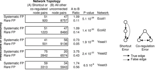
We investigated whether certain struc-tural features of the gold standard net-works led the community to incorrectly predict edges where there should be none. When multiple teams make the same false positive error, we call it a systematic false positive. The number of teams that make the error is a measure of confusion of the community. An ever-present conundrum in network inference is how to discrimi-nate direct regulation from indirect regu-lation. We hypothesized that two types of topological properties of networks could be inherently confusing, leading to system-atic false positives. The first type is what we call shortcut errors, where a false positive shortcuts a linear chain. A second type of direct/indirect confusion is what we call a regulation error, where co-regulated genes are incorrectly predicted to regulate one another (see schematic associated with Figure 7).

Table 9.Results of thein silicosize 100 network inference challenge.

AUROC AUPR Overal

Team p-value p-value Score

B Team 310{71 ₀ _Inf

Bonneau 310{36 ₄₁₀{56 _45.44

IntigernHSP 310{38 ₁₁₀{47 _42.24

Team 305 210{33 ₈₁₀{32 _31.88

Team 301 110{8 ₈₁₀{17 _11.99

Team 310 110{4 ₂₁₀{14 _8.83

Team 314 810{5 ₃₁₀{14 _8.81

Team 183 810{13 ₄₁₀{5 _8.25

Team 254 110{8 ₂₁₀{8 _7.83