On a Class of Statistical Distance Measures for Sales
Distribution: Theory, Simulation and Calibration
Tianhao Wu
Department of Statistics, Yale University, New Haven, CT 06511, USA, E-mail: [email protected]
Abstract While firm-level and micro issue analysis become an important part in research of international trade, only a few work is concerned about the goodness-of-fit for size distribution of firms. In this paper, we revisit the statistical aspects of firm productivity and sales revenue, in order to compare different definitions of statistical distances. We first deduce the exact form of size distribution of firms by only implementing the assumptions of productivity and demand function, and then introduce the famous g-divergence as well as its statistical implications. We also do the simulation and calibration so as to compare those different divergences, moreover, tests the combined assumptions. We conclude that minimizing Pearson χ2and Neyman χ2 produces similar results and minimizing Kullback-Leibler divergence is likely to take the expense of other distance measures. Additionally, selection among different statistical distances is much more significant than demand functions.
Key words Pareto distribution, log-normal distribution, demand function, statistical divergence, firm productivity, sales revenue
JEL Codes: C13, C46, F14
1. Introduction
Starting from the pioneering work by Melitz (2003), who developed a dynamic industry model with heterogeneity to analyze the intra-industry effects, firm-level analysis has become a mainstream research topic in international trade. To the extent that empirical implications have been of concern, trade theory has been aiming at understanding aggregate evidence on such topics as the factor content of trade and industry specialization (Bernard et al., 2003). From this perspective, many studies have also been done in understanding the micro issues, for example, the impact of firm size on productivity.
the assumption of productivity, the distribution of sales can be determined by technology and interaction between firm and consumers. From a theoretical and statistical perspective, CES (Constant Elasticity of Substitution) expenditure function bridges the Pareto distributions of productivity and sales, and the Log-Normal distributions of productivity and sales (Helpman et al., 2004; Head et al., 2014; Mrazova et al., 2016), though the equilibrium resulting in Log-Normal firm size has not been deduced yet. There is also some more detailed work examining the validity of Pareto and Log-Normal sales distribution, for example, Stanley et al. (1995) used a Zipf plot to demonstrate that the upper tail of the size distribution of firms is too thin relative to the log normal rather than too fat.
Jumping from the scope of international trade, some empirical studies focus on fitting the actual sales. Cabral and Mata (2003) demonstrated the right-skewness of firm size distribution using Portuguese manufacturing data. And Brynjolfsson et al. (2014) studied the changes in the shape of Amazons sales distribution curve as well as its impact on consumer surplus gains.
Nevertheless, little literature is concerned about the goodness-of-fit for size distribution of firms. Mrazova et al. (2016) used KLD (Kullback Leibler Divergence) to measure the distances between estimated density and theoretical density, in order to test a new demand function developed by them, called CREMR. In fact, testing and measuring the statistical distance between the empirical distribution and the estimated distribution is of great importance if we want to test the combined assumptions, at least from a statistical standpoint.
Unavoidably, talking about the statistical distance involves the measure of statistical divergence, which is distinguished from the traditional Euclidean distance in metric space. In this paper, we introduce the well-known g-divergences that are applied widely in statistics and engineering. To our surprise, this has not been used too much in economics, in spite of its great properties in measuring the distances.
We start from the assumption of firm productivity, either Pareto or Log-Normal distributions that are proved to be very effective and empirically practical. By combining the assumptions of firm with different forms of demand systems, which further imply the exact forms of the probability distribution of firm sizes. Besides the theory, we also run simulations to get a sense of how those different g-divergences work, concluding that minimizing Pearson χ2 and Neyman χ2 produces similar results and minimizing
2. Sales Distribution
Without assumptions on demand and technological constrains, firm characteristics can be linked by a behavior function by only assuming that characteristics of each firm are monotonically increasing on the number of firms, thus a hypothetical dataset of a continuum of firms (Mrazova et al., 2016). Implementing this assumption, when the linked demand function and the distribution of productivity are specified, sales distribution can be determined statistically. In this section, we use three kinds of demand systems to extract the exact forms of sales distribution by assuming that firm productivity is either distributed Pareto or Log-Normal.
2.1. Pareto productivity
Suppose that the productivity ' is distributed Pareto with scale parameter and shape parameter α, so the cumulative probability function is
From the perspective of pro t-maximization, marginal cost equals marginal revenue. As a result, we can link sales r and productivity by , where x is the output. Accordingly, demand function indeed plays the role of bridging productivity and firm size.
We first give an example of how to deduce the size distribution of firms by using Constant Elasticity of Substitution demand function. Suppose the inverse CES demand function takes the form , we can utilize sales revenue to express firm productivity by the following steps,
Then by the variable transformation, we know that the cumulative probability function of sales is under the setting of CES demand function.
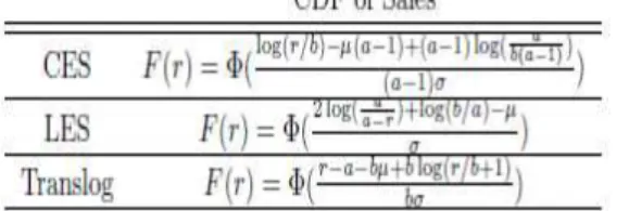
Table 1 summarizes the expression of productivity by sales as well as the sales distribution by three common classes of demand systems.
Table 1. Sales distribution with Pareto distribution of productivity
While we don't provide the exact steps for extracting the sales distributions with LES and Translog demand functions, it's not hard to justify the above table by using the algorithm developed for CES type. Moreover, though we just consider CES, LES and Translog here, in fact, CREMR, Linear and AIDS fall into the same forms of the sales distributions respectively (Mrazova et al., 2016).
2.2. Log-Normal productivity
This section assumes Log-Normal distribution of productivity with location parameter µ and scale parameter σ, so the CDF is
Where Φ is the cumulative probability function of a standard normal random variable. The way of extracting the sales distributions is similar to the last section. When the forms of demand functions and the expressions of firm productivity by firm size do not depend on the distribution of productivity, we only report the sales distributions in the table 2 below.
Table 2. Sales Distribution with Log-Normal distribution of productivity
We express the sales distributions by using the original parameters in demand functions and distributions of productivity. However, sufficient parameters in each distribution are less than those in the table. For example, for the combination of LES with Pareto case, we can express the sales distribution by
1
Accordingly, estimating m; k and h instead of ; a; b and α is sufficient to know the exact distribution of sales. We call it a generalization of parameters and will use the generalized ones for estimation in the next two sections.
3. Statistical divergences
Statistical divergences are used to measure the "distance" between two probability distributions. The importance of suitable measures of distance arises of the role play in the problems of inference and discrimination (Ullah, 1996). While the concepts of statistical distances are not widely applied in Economics, experts in other fields have appreciated them in other fields. For instance, different distances are used to identify the relation between texts of DNAs, planetary nebulae and unitary transformations (Pevzner, 1991; Steene and Zijlstra, 1994; Acin, 2001). In this section, we overview an important class of statistical divergences which is crucial in this paper.
3.1. g-Divergence
Suppose f is the actual (empirical) density and f is the estimated density. The g-divergence22 is defined as
Where g(.) is an arbitrary convex function. The g-divergence is characterized as a unique family of convex separable divergence that satisfies the information monotonicity property (Amari, 2009; Amari and Nagaoka, 2000). The g-divergence is not necessary a metric since the symmetric property is not satisfied for every g, i.e.
Although considering this general form is promising, we need the analytical expression of distances in order to do parametric estimations. As a matter of fact, this class of divergences by defining different g functions have explicit statistical meanings. In this paper, we will mainly use the following.
3.1.1. Kullback-Leibler divergence
Define g(x) = -log(x), then the divergence becomes
2 Some papers name it as f-divergences, such as Nielsen and Nock (2013). But in order not to conflict with the notations of density, we use g here.
(2)
It's the famous Kullback-Leibler Divergence (Relative Entropy). Since minimizing KLD is equivalent to maximizing the Likelihood function, KLD estimators are just MLEs. By this property, KLD might be the most widely used divergence, for example, Mori et al. (2005) used this measure to define industrial localization and Rohde (2016) studied income inequality based on a symmetric extension of KLD.
3.1.2. Pearson and Neyman χ2
Defining g(x) = (x-1)2 and g(x) = (1-x)2 gets Pearson and Neyman χ2 estimators:
sau
These two estimators are applied to sets of categorical data to evaluate how likely it is that any observed difference between the sets arose by chance, which is known as χ2
test.
3.1.3. Total variation distance
If we define , we can get the divergence By this definition, the divergence is symmetrical, i.e.
3.2. Other divergences
In fact, there are a lot of statistical distances that can be considered without restriction to g-divergences. As a robustness check and comparison, we will also use Kolmogorov-Smirnov Statistic and Hellinger Distance in the next two sections. Kolmogorov-Smirnov Statistic is defined as , where F and are the true and estimated cumulative probability functions with respect to f and . Furthermore, Hellinger Distance is , to which square is in g-divergences class.
4. Simulation
Firm productivity and sales revenue are fitted by Pareto and Log-Normal distribution in many studies. Consequently, by the importance of these two probability distributions, this section presents the simulated results of Pareto and Log-Normal variables. Specifically, we simulate a set of values drawn from either
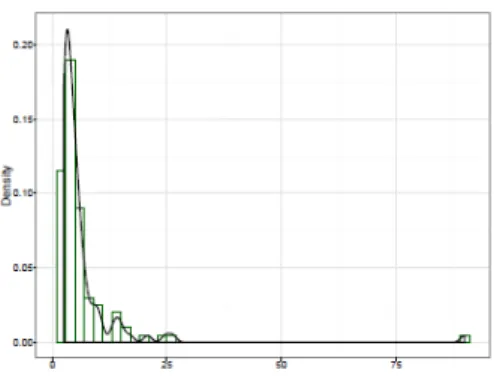
4.1. Pareto simulation
In this section, we simulate Pareto variable with scale parameter 2.5 and shape parameter 1.5. Figure 1 is the histogram with density of our simulated data.
Figure 1. Pareto
In order to estimate the parameter, we minimize over each definition of statistical distance and report them for each different optimization.
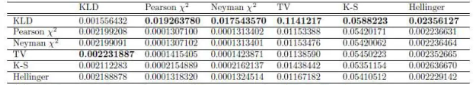
Table 3. Distances between predicted density and actual density for Pareto
The first column represents the minimized distance and each row stands for the estimated values with correspondence to the rule in the left.
4.2. Log-Normal simulation
Figure 2. Log-Normal
Again by minimizing different statistical divergences, we have the following summary table.
Table 4. Distances between predicted density and actual density for Log-Normal
4.3. Discussions
Cross-comparison may be of little interest, but we can compare the values within the same distance group. We notice that minimizations of Pearson χ2, Neyman χ2 and total
variation distance give similar estimated results with respect to all different measures and both for Pareto and Log-Normal simulations. Furthermore, such similarity is even larger for minimizing Pearson χ2 and Neyman χ2. Also the estimated Pearson χ2 and
Neyman χ2 are pretty close under each rule. While it's easy to see from the forms of
those two χ2 estimators that their definitions are actually highly related and when the
estimated density approximates the true density, they are closer, we do not have any powerful explanations for why TV method is also similar.
variation33. So we would expect a stable performance for K-S estimations. Moreover,
KLD estimation method looks different from others, if we remove the row of KLD in the table, we can easily discover large stability of all estimators. From these perspectives, KLD and K-S distances may not be very good ones since they minimize KLD and K-S respectively by taking the expense of other distances. We can conclude that more obviously by look at the bold numbers which are the maximum of each column.
5. Calibration
In this section, we do a calibration to show how the concepts of g-divergences can test economics assumptions, at least from a statistical perspective. Certainly, each market can be modeled by a mixture of demand systems. And the specification of demand system associate with the assumption of firm productivity can determine the distribution of sales, which further determines the behavior of sales. However, traditional economics methods fall into regression to fit sales data, hence testing whether the assumptions hold, for example, see Tobin (1950); Bergstrom and Goodman (1973); Griliches (1958). Intuitively, smaller the statistical distances are, the more approximation of the predication, resulting in more reasonable assumptions.
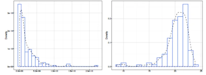
We give an example of how these work. To be specific, we use aggregate manufacturer-level sales data exported from US to Canada in 2015, which can be found via US Census Bureau Economic Statistics. We will mainly focus on the performances of different demand settings and the firm productivity assumptions. Figure 3 below are two histograms with density plot, the right one is after taking logarithm transformation.
Figure 3. Histograms
3
At the first glance, either Pareto or Log-Normal is likely to fit the data well. Then we turn to the g-divergences estimations, table 5 below reports the estimated divergences under two different assumptions of productivity and multiple demand settings. For example, the entries of the Translog column in the Pareto suitable mean the minimized values of those six divergences. And we make the minimums in each row bold.
Table 5. Distances between predicted density and actual density for selected demand functions
function, things are opposite other than Pearson χ2 estimation. Finally, we note that the
differences between the selections of divergence measure are certainly less significant than demand functions. Or say, the differences between columns are much less than the differences between rows, which are an evidence of the importance of choosing statistical measures. However, this is just a simple calibration example which illustrates how to compare the assumption in the market of U.S. exporting to Canada. Economics networks can be hugely complicated and cannot be fuelled explained with very simple assumptions. Also, sales data are of course not drawn from a completely random process. Thus we do not have a dinner table yet to discuss the underlying difference among distances and how to predict the sales distribution generally.
6. Conclusions
With firm-level analysis playing an essential role in international trade research, understanding micro issues such as firm productivity and firm size are not only important for theory development but also empirically useful. In this paper, we revisit the statistical perspectives of productivity and firm sales and use an efficient tool to compare different statistical divergences as well as assumptions of firm and demand functions. The simulation results show that Pearson χ2 and Neyman χ2 perform pretty
similar and minimizing Kullback-Leibler divergence is likely to be at the expense of other distance measures. We also do a calibration on manufacturer-level data exported from US to Canada in 2015. From the empirical results, we conclude that Translog is the most impossible one to fit the demand system in the example. Moreover, we conclude that selection among different statistical distances is much more significant than different demand functions. We emphasis our work as the one of few papers studying the goodness-of-fit problem in predicting size distribution of firms, from an empirically statistical standpoint. Also, we do think more work can be done on this topic such like how to use the divergence tool to test economics assumptions.
References
Acin, A. (2001). Statistical distinguishability between unitary operations. Physical Review Letters 87 (17), 1-4.
Amari, S., Nagaoka, H., (2000). Methods of information geometry. Oxford University Press.
Amari, S.-I., (2009). Alpha-divergence is unique, belonging to both f-divergence and bregman divergence classes. IEEE Transactions on Information Theory 55 (11), 4925-4931.
Bee, M., Riccaboni, M., Schiavo, S., (2014). Where gibrat meets zipf: Scale and scope of french firms. DEM Discussion Papers.
Bergstrom, T.C., Goodman, R.P., (1973). Private demands for public goods. The American Economic Review 63 (3), 280-296.
Bernard, A. B., Eaton, J., Jensen, J. B., Kortum, S., (2003). Plants and productivity in international trade. American Economic Review 93 (4), 1268-1290.
Brynjolfsson, E., Hu, Y. J., Smith, M. D., (2014). The longer tail: The changing shape of amazon's sales distribution curve. Available at SSRN: http://ssrn.com/
abstract=1679991.
Cabral, L. M. B., Mata, J., (2003). On the evolution of the _rm size distribution: Facts and theory. The American Economic Review 4 (1), 1075-1096.
Griliches, Z., (1958). The demand for fertilizer: An economic interpretation of a technical change. Journal of Farm Economics 40 (3), 591-606.
Head, K., Mayer, T., Thoenig, M., (2014). Welfare and trade without Pareto. The American Economic Review 104 (5), 310-316.
Helpman, E., Melitz, M.J., Yeaple, S. R., (2004). Export versus FDI with heterogeneous firms. The American Economic Review 94 (1), 300-316.
Melitz, M., (2003). The impact of trade on intra-industry reallocations and aggregate industry productivity. Econometrica 71, 1695-1725.
Mori, T., Nishikimi, K., Smith, T.E., (2005). A divergence statistics for industry localization. The Review of Economics and Statistics 87(4), 635-651.
Mrazova, M., Neary, J.P., Parenti, M., (2016). Sales and markup dispersion: Theory and empirics. Working Paper.
Nielsen, F., Nock, R., (2013). On the chi square and higher-order chi distances for approximating -divergences. IEEE Signal Processing Letters.
Pevzner, P.A., (1991). Statistical distance between texts and filtration methods in sequence comparison. Bioinformatics 8 (2), 121-127.
Rohde, N., (2016). J -divergence measurements of economic inequality. Journal of the Royal Statistical Society: Series A (Statistics in Society) 179 (3), 847-870.
Stanley, M. H., Buldyrev, S. V., Havhn, S., Mantegna, R. N., Salinger, M. A., Stanley, H. E., (1995). Zipf plots and the size distribution of firms. Economics Letters 49, 453-457.
Steene, G.C.V., Zijlstra, A.A., (1994). On an alternative statistical distance scale for planetary nebulae. Astronomy and Astrophysics Supplement Series 108, 484-490. Tobin, J., (1950). A statistical demand function for food in the u.s.a. Journal of the Royal Statistical Society. Series A (General) 113 (2), 113-149.