EPQ model for imperfect production processes with rework and random preventive machine time for deteriorating items and trended demand

25 (2015), Number 3, 425-443 DOI: 10.2298/YJOR130608019S

EPQ MODEL FOR IMPERFECT PRODUCTION

PROCESSES WITH REWORK AND RANDOM

PREVENTIVE MACHINE TIME FOR DETERIORATING

ITEMS AND TRENDED DEMAND

Nita H. SHAH

Department of Mathematics, Gujarat University, India 1_{nitahshah@gmail.com}

Dushyantkumar G. PATEL

Department of Mathematics, Govt. Poly.for Girls, India dushyantpatel_1981@yahoo.co.in

Digeshkumar B. SHAH

Department of Mathematics, L. D. College of Engg., India digeshshah2003@yahoo.co.in

Received: July 2013 / Accepted: July 2014

Abstract: Economic production quantity (EPQ) model is analyzed for trended demand and the units which are subject to constant rate of deterioration. The system allows rework of imperfect units and preventive maintenance time is random. The proposed methodology, a search method used to study the model, is validated by a numerical example. Sensitivity analysis is carried out to determine the critical model parameters. It is observed that the rate of change of demand and the deterioration rate have a significant impact on the decision variables and the total cost of an inventory system. The model is highly sensitive to the production and demand rate.

Keywords: EPQ, Deterioration, Time-dependent Demand, Rework, Preventive Maintenance, Lost Sales.

MSC: 90B05.

1. INTRODUCTION

phenomenon is known as rework, Schrady(1967). At manufacturer‟s end, the rework is advantageous because this will reduce the production cost. Khouja (2000) modeled an optimum procurement and shipment schedule when direct rework is carried out for defective items. Kohet al. (2002) and Dobos and Richter (2004) discussed two optional production models in which either opt to order new items externally or recover existing product. Chiu et al. (2004) studied an imperfect production processes with repairable and scrapped items. Jamal et al. (2004), and later Cardenas – Barron (2009) analyzed the policies of rework for defective items in the same cycle and the rework after N cycles. Teunter (2004), and Widyadana and Wee (2010) modeled an optimal production and a rework lot-size inventory models for two lot-sizing policies. Chiu (2007), and Chiu et al. (2007) incorporated backlogging and service level constraint in EPQ model with imperfect production processes. Yoo et al. (2009) studied an EPQ model with imperfect production quality, imperfect inspection, and rework.

The rework and deterioration phenomena are dual of each other. In other words, the rework processes is useful for the products subject to deterioration such as pharmaceuticals, fertilizers, chemicals, foods etc., that lose their effectivity with time due to decay. Flapper and Teunter (2004), and Inderfuthet al. (2005) discussed a logistic planning model with a deteriorating recoverable product. When the waiting time of rework process of deteriorating items exceeds, the items are to be scrapped because of irreversible process. Wee and Chung (2009) analyzed an integrated supplier-buyer deteriorating production inventory by allowing rework and just-in-time deliveries. Yang et al. (2010) modeled a closed-loop supply chain comprising of multi-manufacturing and multi-rework cycles for deteriorating items. Some more studies on production inventory model with preventive maintenance are by Meller and Kim (1996), Sheu and Chen (2004), and Tsou and Chen (2008).

Abboudet al (2000) formulated an economic lot-size model when machine is under repair resulting shortages. Chung et al. (2011), Wee and Widyadana (2012) developed an economic production quantity model for deteriorating items with stochastic machine unavailability time and shortages.

2. ASSUMTIONS AND NOTATIONS

2.1.Assumptions

1. Single item inventory system is considered.

2. Good quality items must be greater than the demand. 3. The production and rework rates are constant.

4. The demand rate, (say)R( t ) a( 1bt )is function of time where a0is scale demand and 0 b 1denotes the rate of change of demand.

5. The units in inventory deteriorate at a constant rate; 0 



1.

6. Set-up cost for rework process is negligible or zero.

7. Recoverable items are obtained during the production up time and scrapped items are generated during the rework up time.

2.2 Notations

1a

I : serviceable inventory level in a production up time

2a

I : serviceable inventory level in a production down time

3a

I : serviceable inventory level in a rework up time

3r

I : serviceable inventory level from rework up time

4r

I : serviceable inventory level from rework process in rework down time

1 r

I : recoverable inventory level in a production up time

3 r

I : recoverable inventory level in a rework up time

1a

TI : total serviceable inventory in a production up time

2a

TI : total serviceable inventory in a production down time 3a

TI : total serviceable inventory in a rework up time 3r

TI : total serviceable inventory from a rework up time 4r

TI : total serviceable inventory from rework process in a rework down time

1

r

TTI : total recoverable inventory level in a production up time

3 r

TTI : total recoverable inventory level in a rework up time

1a

T : production up time

2a

T : production down time

3r

T : rework up time

4r

T : rework down time

sb

T : total production down time

1aub

T

: production up time when the total production down time is equal to the

m

I

: inventory level of serviceable items at the end of production up time

mr

I

: maximum inventory level of recoverable items in a production up time

w

I

: total recoverable inventory

P

: production rate 1

P : rework process rate

 

RR t : demand rate; a



1bt



,a0, 0 b 1

x

: product defect rate

1

x

: product scrap rate

 : deteriorate at a constant rate ;0 



1.

A

: production setup cost

h

: serviceable items holding cost

1

h

: recoverable items holding cost

C

S

: scrap cost

L

S : lost sales cost

d

C : Cost of deteriorated units

TC : total inventory cost T : cycle time

TCT : total inventory cost per unit time for lost sales model

NL

TCT : total inventory cost per unit time for without lost sales model

U

TCT : total inventory cost per unit time for lost sales model with uniform distribution preventive maintenance time

E

3. MATHEMATICAL MODEL

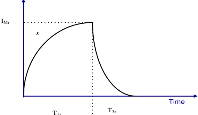
The rate of change of inventory is depicted in Figure1.During production period0,T₁a,

x

defective items per unit time are to be reworked. The rework process starts at the end of time

T

_1a. The rework time ends at

T

_3r time period. The production rates of good items and defective items are different. During the rework process, some recoverable and some scrapped items are obtained. LIFO policy is considered for the production system. So, serviceable items during the rework up time are utilized before the fresh (new) items from the production up time. The new production cycle starts when the inventory level reaches zero at the end of

T

_2atime period. Because machine is under maintenance, which is randomly distributed with probability density function f t ,

 

the new production cycle may not start at timeT_2a. The production down time may result in shortage T₃- time period. The production will start after theT₃time period.

Time Inventory level

Im

T1a T3r T4r T2a

T1 T2

T3

T

Figure 1: Inventory status of serviceable items with lost sales

Under above mentioned assumptions, the inventory level during production up time can be described by the differential equation

 

_{ }

_{ }

1 1

1 1 1 1 1

1

0

a a

a a a a a

a

d I t

P R t x I t , t T

dt       (1)

The inventory level during rework up time is governed by the differential equation

 

_{ }

_{ }

3 3

1 3 1 3 3 3 3

3

0

r r

r r r r r

r

d I t

P R t x I t , t T

dt       (2)

 

_{ }

_{ }

2 2

2 2 2 2 2

2

0

a a

a a a a a

a

d I t

R t I t , t T

dt      (3)

and during rework down time is

 

_{ }

_{ }

4 4

4 4 4 4 4

4

0

r r

r r r r r

r

d I t

R t I t , t T

dt      (4)

Under the assumption of LIFO production system, the rate of change of inventory of good items during rework up time and down time is governed by

 

_{ }

3 3

3 3 3 3 4

3

0

a a

a a a r r

a

d I t

I t , t T T

dt     

(5)

UsingI1a

 

0 0, the inventory level in a production up time is

 







1





1



1 1 2 1

1

1 ta ta 1

a a a

ab

I t P a x e e



t





 

      

(6) The total inventory in a production up time is

 

1

1 1 1 1

0 a

T

a a a a

TI   I t dt

(7)

Using, I_3r

 

0 0, solution of (2) is

 







3





3



3 3 1 1 2 3

1

1 tr tr 1

r r r

ab

I t P a x e e



t





 

       (8)

and total inventory in a rework up time is

 

3

3 3 3 3

0 r

T

r r r r

TI   I t dt (9)

Using I_4r

 

t_4r 0, solution of (4) is

 



4 4

 

4 4

 

4 4



4r 4r ( Tr tr) 1 ₂ ( Tr tr) 1 4r ( Tr t r) 1

a ab ab

I t e e T e

  _   

      (10)

And hence the total inventory of serviceable items during rework down time is

 

4

4 4 4 4

0 r T

r r r r

TI 



I t dt (11)

 

2

2 2 2 2

0 a T

a a a a

TI 



I t dt (12)

Now, the maximum inventory level is

 







1





1



1 1 2 1

1

1 Ta Ta 1

m a a a

ab

I I T P a x e e T

 

 

       

(13) Hence, the total inventory in a rework up time is





2

3 3 4 3 4

2

a m r r r r

TI I _T T  T T _

  (14)

Next, we analyze the inventory level of recoverable items. (Figure

Time IMr

T1a T3r

x

Figure 2: Inventory status of recoverable items The rate of change of recoverable items in a production up time is

 

_{ }

1 1

1 1 1 1

1

, 0

r r

r r r a

r

d I t

x I t t T

dt  



  (15)

Using Ir₁

 

0 0 , the inventory level of the recoverable items during the production up time is

 



1



1 1 1 r , 0 1 1

t

r r r a

x

I t e t T





   

(16)

hence, total recoverable items in a production up time is

1

1 1 1 1

0 ( )

a T

r r r r

TTI 



I t dt

Initially, the recoverable inventory is

 



1



1 1 1

2 1 1 1 2 a T

Mr r a a

a a

x

I I T e T

T x T 





       _  _   (18)

The rate of change of inventory level of recoverable item during the rework up time is governed by differential equation

 

_{ }

3 3

1 3 3 3 3

3

, 0

r r

r r r r

r

d I t

P I t t T

dt   



  (19)

Using, Ir3

 

t3r 0, the solution of equation (19) is

 

1



 3 3



3 3 1

r r T t r r

P

I t e





  (20)

The total inventory of recoverable item during rework up time is

3

3 3 3 3

0 ( )

r T

r r r r

TTI 



I t dt

(21)

The number of recoverable items is

 

1



3



3 0 r 1

T

Mr r

P

I I e



   (22)

Since T_3r 1 and using Taylor's series approximation, equation (22) gives

3 1 Mr r I T P  (23)

Substituting

I

_Mr from equation (18) in equation (23), we get

2 1 3 1 1 2 a r a T x T T P



   _  _

  (24)

Total recoverable items

1 3

w r r

I TTI TTI (25)

 

 

 

1 3 2 4

1 1 3

0 0 0

a r a r

T T T T

r

DU P R t dt P R t dt R t dt x T



   

_   _{ }  _ 





 







(26)

Since the inventory level at the beginning of the production down time is equal to the inventory level at the end of the production up time minus the deteriorated units at

3r 4r

T T , using Misra(1975), the approximation concept, we have





2









2

2 1 1 3 4 3 4

1 1

1

2 2

a a a r r r r

ab

T P a x T T T T T T

a  

   

 _    _{ }     _

    (27)

The inventoryfor serviceable item in rework process is

 

 

3r 3r 4r 0

I T I

by simple calculations





4 1 1 3 3

1 1

1 2

r r r

T P a x T T

a 

 

   _  _

  (28)

Using equations (24) and (28), T_2a given in equation (27) is only a function of T_1a. The total production cost of inventory system is sum of production set up cost, holding cost of serviceable inventory, deteriorating cost of recoverable inventory cost, and scrap cost.

Therefore,

1a 3r 2a 4r 3a 1 w d C 1 3r

TC A h TI_ TI TI TI TI _h I C DUS x T (29) total replenishment time is

1a 3r 2a 4r

TT T T T (30)

The total cost per unit time without lost sales is given by

NL TC TCT

T

 (31)

The optimal production up time for the EPQ model without lost sales is the solution of

 

1

1

0

NL a

a

dTCT T

dT  (32)

 

 









 

2 4

2 4

a r

L a r

t T T

E TC TC S R t t T T f t dt



 

 

_

  (33)

the total cycle time for lost sales scenario is

 

_





_

 

2 4

2 4

a r

a r

t T T

E T T t T T f t dt



 

 



  (34)

Using equations (33) and (34), the total cost per unit time for lost sales scenario is





E TC

 

_{ }

E TCT

E T

 (35)

3.1. Uniform distribution Case

Define the probability distribution function f t

 

, when the preventive maintenance time

t

follows uniform distribution as follows.

 

1, 0 0, otherwise

t

f t  

 _{ }

   

substituting f t

 

in equation (35) gives total cost per unit time for uniform distribution as

















1 3 2 4 3 1 1 3 2 4

0

1 3 2 4 2 4

0

(1 )

1

L

a r a r a w d C r a r

U

a r a r a r

S

A h TI TI TI TI TI h I C DU S x T a bt t T T dt

TCT

T T T T t T T dt

     _     _             





(36)

The optimal production up time for lost sales case is solution of

 

1

1

0

U a

a

dTCT T

dT  (37)

To decide whether manufacturer should allow lost sales or not, we propose following steps (Wee and Widyadana (2011)):

Step 1: Calculate T1a from equation (32). Hence calculate T2a from equation (27) and

4r

T from equation (28). Set TsbT2aT4r.

Step 3: Set T_sb . Find T1aub using equations (27) and (28). Calculate



1



NL aub

TCT T using equation (31).

Step 4: Calculate T_1a from equation (37), hence T_2afrom equation (27) and T_4r from equation (28), and set TsbT₂aT₄r.

Step 5: If T_sb then optimal production up time T_1a is T_1aub and



1



NL aub

TCT T IfT_sb, then, calculate TCT_U

 

T_1a using equation (36).

Step 6: If TCT_NL



T_1aub



TCT_U

 

T_1a , then optimal production up time T_1aub; otherwise it is

T

_1a

3.2. Exponential distribution case

Define the probability distribution function f t

 

, when the preventive maintenance time

t

_{follows exponential distribution with mean} 1

 as

 

t, 0.

f t 



e





Here, the total cost per unit time for lost sales scenario is

 









 

2 4

2 4

2 4

1 a r

a r

t

L a r

t T T E

T T

TC S R t t T T e dt

TCT

T e











  

 

  







(38)

The optimal T1acan be obtained by setting

 

1 1

0

E a

a

dTCT T

dT  (39)

The convexity of TCT_NL,TCT_U and/or TCT_Ehas been established graphically with suitable values of inventory parameters.

4. NUMERICAL EXAMPLE AND SENSITIVITY ANALYSIS

In this section, we validate the proposed model by numerical example. First, we consider uniform distribution case. Take A$200 per production cycle,

10,000

P units per unit time, P14000units per unit time,a5000units per unit time, 10%

unit time. h1$3 per unit per unit time, SL$10 per unit, SC $12 per unit,

$0.01

d

C  per unit ,



10% and the preventive maintenance time is uniformly distributed over the interval



0, 0.1 . Following algorithm with Maple 14, the optimal



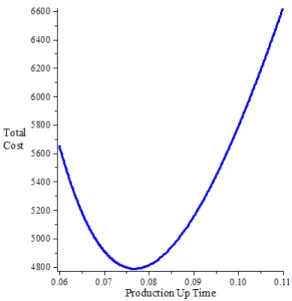
production up time T₁a0.109years and the corresponding optimal total cost per unit time is TCTU $4448. The convexity of TCTUis exhibited in Figure 3.

Figure 3: Convexity of Total Optimal Cost with Uniform Distribution The sensitivity analysis is carried out by changing one parameter at a time by 40%, 20%, 20% and 40%

    . The optimal production up time and the total cost per unit time for different inventory parameters are exhibited in Table 1.

Table 1 Sensitivity analysis of T1a and total cost when preventive maintenance time for

Parameter Percentage change Uniform Distribution Exponential Distribution λ = 20

T1a TCT T1a TCT

A

-40% 0.107791969 4078.521832 0.139574511 5113.723713 -20% 0.108600011 4263.884212 0.139810498 5115.079416 0 0.10940717 4447.906835 0.140048682 5116.43044 20% 0.110213455 4630.606199 0.140289094 5117.776849 40% 0.111018878 4811.998518 0.140531765 5119.118693

P

-40% Not Feasible Not Feasible 0.80333702 4497.769808 -20% 0.191001903 4040.012884 0.230211542 4821.961079 0 0.10940717 4447.906835 0.140048682 5116.43044 20% 0.076808684 4787.228599 0.101644181 5282.346729 40% 0.059274011 5086.939301 0.08003233 5389.345959

P1

-40% 0.118683393 4700.523848 0.146305758 5506.08129 -20% 0.11269291 4526.771856 0.14232037 5258.800083 0 0.10940717 4447.906835 0.140048682 5116.43044 20% 0.107362559 4412.358408 0.138580965 5023.818806 40% 0.105989146 4400.192947 0.137554578 4958.738514

A

-40% Not Feasible Not Feasible 0.065854221 3719.215509 -20% 0.07246471 4196.531895 0.097126915 4449.530627 0 0.10940717 4447.906833 0.140048682 5116.43044 20% 0.16785454 4733.262382 0.204019241 5718.553561 40% 0.273755232 5081.486552 0.314035664 6269.664841

B

-40% 0.109157125 4445.377023 0.13955077 5104.426062 -20% 0.10928183 4446.642683 0.139799146 5110.431143 0 0.10940717 4447.906833 0.140048682 5116.43044 20% 0.109533149 4449.169487 0.140299393 5122.423958 40% 0.109659774 4450.430641 0.140551295 5128.411696

X

Parameter Percentage change Uniform Distribution Exponential Distribution λ = 20

T1a TCT T1a TCT

-40% 0.109193541 4386.01374 0.139884967 5054.344838 -20% 0.109300267 4416.943204 0.139966795 5085.371346 0 0.10940717 4447.906833 0.140048682 5116.43044 20% 0.109514249 4478.904682 0.140130627 5147.5222 40% 0.109621504 4509.936823 0.14021263 5178.646666

h

-40% 0.111814445 3929.608716 0.150159236 4453.225302 -20% 0.110597091 4190.190873 0.144782689 4790.825835 0 0.10940717 4447.906833 0.140048682 5116.43044 20% 0.108243755 4702.808287 0.135826709 5431.367706 40% 0.107105962 4954.945599 0.132021882 5736.710556

h1

-40% 0.109492258 4429.380983 0.140379577 5093.016012 -20% 0.109449696 4438.645749 0.140213774 5104.730522 0 0.10940717 4447.906833 0.140048682 5116.43044 20% 0.109364678 4457.164251 0.139884294 5128.115837 40% 0.10932222 4466.417991 0.139720605 5139.78676

SL

-40% 0.106222274 4429.303489 0.122003914 4700.202185 -20% 0.108157269 4440.669141 0.131984403 4930.302135 0 0.10940717 4447.906833 0.140048682 5116.43044 20% 0.110281085 4452.91983 0.146835261 5273.171982 40% 0.110926483 4456.597219 0.152705659 5408.808796

Sc

-40% 0.10941866 4327.54245 0.140134136 4997.933007 -20% 0.109412921 4387.724673 0.140091431 5057.182213 0 0.10940717 4447.906833 0.140048682 5116.43044 20% 0.109401406 4508.088927 0.140005888 5175.677688 40% 0.109395631 4568.270952 0.13996305 5234.923957

Θ

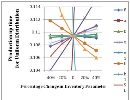
Figure 4: Sensitivity analysis of production up time for uniform distribution

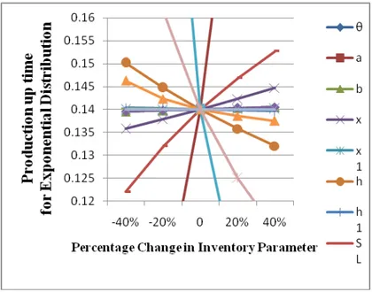
Figure 6: Sensitivity analysis of production up time for exponential distribution

Figure: 7 Sensitivity analysis of total cost for exponential distribution

changes in other parameters. T1ais negative related to Pand



and positively related to

a

_and T1a. Figure 6 exhibits variations in the optimal total cost per unit time with

uniform distribution. The optimal total cost is slightly sensitive to changes in , , , _d

a P x C andh; moderately sensitive to changes in A, , Sc, , x1and SLand insensitive

to changes in other parameters.

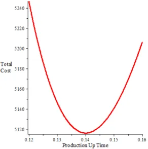
Take mean of exponential distribution as 20. The optimum total cost is $ 5116 when the optimal production up time is 0.14 years. The convexity of the total cost is shown in Figure 8.

Figure 8: Convexity of Total Optimal Cost with Exponential Distribution From Figure6, for lost sales with exponential distribution, it is observed that the optimal production up time is slightly sensitive to changes in

P

_and a, moderately sensitive to changes in the parameter



and



, and insensitive to changes in other parameters. The optimal production up time is negatively related to ,P band



, and positively related to the value of

a

.

In Figure7, variations in the optimal total cost is studied. Observations are similar tothe uniform distribution case.

5. CONCLUSIONS

depute an efficient technician to reduce preventive maintenance time. This model has wide applications in manufacturing sector. Because of using machines for a long period of time,manufacturer facesimproper production, some customers are not satisfied with the quality of the production so, manufacturer has to adopt rework policy.Future research by considering constraints on the machine‟s output, machine‟s life time will be worthy.

Acknowledgements: Authors would like to thank all the anonymous reviewers for their constructive suggestions.

REFERENCES

[1] Abboud, N. E., Jaber, M. Y., and Noueihed, N. A., “Economic Lot Sizing with the

Consideration of Random Machine Unavailability Time”, Computers & Operations Research,

27 (4) (2000) 335-351.

[2] Cardenas-Barron, L. E., “On optimal batch sizing in a multi-stage production system with

rework consideration”, European Journal of Operational Research, 196(3) (2009) 1238-1244.

[3] Chiu, S. W., “Optimal replenishment policy for imperfect quality EMQ model with rework

and backlogging”, Applied Stochastic Models in Business and Industry, 23 (2) (2007)

165-178.

[4] Chiu, S. W., Gong, D. C., and Wee, H.M., “Effect of random defective rate and imperfect

rework process on economic production quantity model”, Japan Journal of Industrial and Applied Mathematics, 21 (3) (2004) 375-389.

[5] Chiu, S.W., Ting, C. K., and Chiu, Y. S. P., “Optimal production lot sizing with rework, scrap

rate, and service level constraint”, Mathematical and Computer Modeling, 46 (3) (2007)

535-549.

[6] Chung, C. J., Widyadana, G. A., and Wee, H. M., “Economic production quantity model for

deteriorating inventory with random machine unavailability and shortage”, International

Journal of Production Research, 49 (3) (2011) 883-902.

[7] Dobos, I., and Richter, K., “An extended production/recycling model with stationary demand

and return rates”, International Journal of Production Economics, 90(3)(2004), 311-323.

[8] Flapper, S. D. P., and Teunter, R. H., “Logistic planning of rework with deteriorating work

-in-process”, International Journal of Production Economics, 88 (1) (2004) 51-59.

[9] Inderfuth, K., Lindner, G., and Rachaniotis, N. P., “Lot sizing in a production system with

rework and product deterioration”, International Journal of Production Research, 43 (7) (2005) 1355-1374.

[10] Jamal, A. M. M., Sarker, B. R., and Mondal, S., “Optimal manufacturing batch size with rework process at a single-stage production system”, Computer & Industrial Engineering, 47 (1) (2004) 77-89.

[11] Khouja, M., “The economic lot and delivery scheduling problem: common cycle, rework, and

variable production rate”, IIE Transactions, 32 (8) (2000) 715-725.

[12] Koh, S. G., Hwang, H., Sohn, K. I., and Ko, C. S., “An optimal ordering and recovery policy

for reusable items”,Computers & Industrial Engineering, 43 (1-2) (2002) 59-73.

[13] Meller, R. D., and Kim, D. S., “The impact of preventive maintenance on system cost and

buffer size”, European Journal of Operational Research, 95 (3) (2010) 577-591.

[14] Misra, R. B., “Optimum production lot-size model for a system with deteriorating inventory”,

International Journal of Production Research, 13 (5) (1975) 495-505.

[15] Schrady, D. A., “A deterministic inventory model for repairable items”, Naval Research Logistics,14 (3) (1967) 391-398.

[16] Sheu, S. H., and Chen, J. A., “Optimal lot-sizing problem with imperfect maintenance and

[17] Teunter, R., „Lot-sizing for inventory system with product recovery”, Computers & Industrial Engineering, 46 (3) (2004) 431-441.

[18] Tsou, J. C., and Chen, W. J., “The impact of preventive activities on the economics of production systems: Modeling and application”, Applied Mathematical Modelling, 32 (6) (2008) 1056-1065.

[19] Wee, H. M., and Chung, C. J., “Optimizing replenishment policy for an integrated production inventory deteriorating model considering green component-value design and

remanufacturing”, International Journal of Production Research, 47 (5) (2009) 1343-1368.

[20] Wee, H. M., and Widyadana, G. A., “Economic production quantity models for deteriorating

items with rework and stochastic preventive maintenance time”, International Journal of

Production Research, 50 (11) (2012) 2940-2952.

[21] Widyadana, G. A., and Wee, H. M., “Revisiting lot sizing for an inventory system with

product recovery”, Computers and Mathematics with Applications, 59 (8) (2010) 2933-2939.

[22] Yang, P. C., Wee H. M., and Chung S. L., “Sequential and global optimization for a closed

-loop deteriorating inventory supply chain”, Mathematical and Computer Modeling, 52 (1-2)

(2010) 161-176.