Time Contingency Assessment in Construction Projects in Egypt using Artificial Neural Networks Model

Time Contingency Assessment in Construction Projects

in Egypt using Artificial Neural Networks Model

Hazem Yahia1_{, Hossam Hosny}2 _{and Mohammad E. Abdel Razik}3 1 _{MSc. Student, Building and Construction Dept., Faculty of Engineering,}

Arab Academy for Science and Technology and Maritime Transport Cairo, Egypt.

2 Associate Professor, Construction Engineering Dept. ,Faculty of Engineering, Zagazig University Zagazig, Egypt

3 _{Professor, Building and Construction Dept., Faculty of Engineering,} Arab Academy for Science and Technology and Maritime Transport,

Cairo, Egypt,

Abstract

Time schedule is an essential tool for construction project management. For instance, it can materially help to identify the expected financial requirements. It is also an important tool for the time control process. Construction project time schedule is greatly affected by many uncertain but predictable factors. Hence, a cer tain percentage of time contingency should be added to the scheduled time to arrive at more reliable time schedule. In this research, the most important factors affecting time contingency in construction projects were identified based on a co mprehensive survey among a co llected sample of the Egyptian construction experts. In addition, a neural networks model was developed in order to help project planner to have a more reliable prediction for the amount of time contingency that should be added to the scheduled completion time. This paper explains the data collection process, lists the main factors affecting time contingency and discusses the model development methodology.

Keywords: Planning, Scheduling,Time, Contingency, , Delay,

Neural.

1.

Introduction

Planning and time schedule is one of the most important tools for construction project management. For instance, it is the base for the project time control. The importance of planning was specified in general as follows: First, to offset uncertainty and change; Second, to focus attention on objectives; Third, to gain economical operation; Fourth, to facilitate control [1]. It has also an important role in cash flow prediction and resources management. One of the major functions of time schedule is the prediction of the expected project completion time. The reliability of such prediction is greatly affected by many uncertain but predictable factors. So, a cer tain time

contingency should be added to the scheduled completion time to arrive at a more reliable prediction for that time. The time contingency is the amount of time added to the base estimated amount to achieve a s pecific confidence level or allow for changes where experience shows obligation [2]. An accurate estimating of time contingency is seen as a m ajor factor for achieving a successful construction projects. Although several industrial sectors developed and used software for estimating time and cost contingencies in order to minimize delays and over budget, yet limited efforts are reported in the literature in the area of predicting time contingency in the construction sector [2].

The objective of this paper is to identify the main factors affecting time contingency based on a co mprehensive survey among a collected samples of construction experts in Egypt. In addition, a neural networks model was developed in order to help project planner to have a more reliable prediction for the amount of time contingency that should be added to the scheduled completion time.

2.

Literature Review

Processes [AHP] to develop a t ime contingency model. Zayed has concluded that the time contingency ranged from 0.167 to 0.778 out of project duration. Thus, the average time contingency of the selected projects is about 35.4% [2]. Second, Park, M. et al. (2004) developed a simulation-based buffering strategy. Reliability buffering aims to generate a robust construction plan that protects against uncertainties by reducing the potential impact of construction changes. The effectiveness of reliability buffering is examined by simulating a d ynamic project model that integrates the simulation approach with the network scheduling approach. The research results indicate that reliability buffering can help achieve shorter project duration without driving up costs by pooling, resizing, relocating, and re-characterizing contingency buffers [3]. Third, Hoffman, G.J. et al. (2007) developed a Multi Layer Regression Model [MLR]. The results suggested that the MLR model is the most useful for its intended purpose: to predict or provide reasonable duration estimate for construction projects. A main benefit of the model is that it does not require a detailed analysis; additionally, it c an also be used as a policy setting tool or to either produce or verify front-end duration estimate [4].

3.

Data Collection

This research aims to identify the main factors which have effects on projects time contingency in the Egyptian construction market. Identifying these factors can help to accurately assessment the required time contingency which should be added to the project planned duration. Eighty four factors were collected based on literature review as shown in Table 1. Such factors were identified based on the work provided by references [5-14].

Based on these factors, two forms of questionnaire were prepared in this research; first, aims to rank the previously identified factors according to their expected impact and probability of occurrence through direct interviews with the Egyptian construction market experts. Then, the most important factors were identified. Second, data gathering sessions were conducted for 54 building construction projects. These projects were executed by class “A” contractors according to classification of the Egyptian Federation for Construction and Buildings Contractors.

Table 1. List of factors affecting time contingency, based on references [5-14]

Ser. Factor Ser. Factor

Project Conditions

1 Project Location 2 Project Design complexity 3 Equipments shortage [Construction technology] 4 Material shortage [Market] 5 Project location [Near from governmental Buildings

i.e. embassies, ministries, .etc] 6 Preparing the plan during project preliminary Stages [i.e. Initiation, Tender phase] 7 Limited time allowed for preparation of the schedule 8 Missing Project Scope Items [conflicts between

project documents].

9 High Level of Quality requirements 10 Lack of Experience in similar projects.

11 Lack of Consultant Experience 12 Unexpected onerous requirements by client’s supervisors [Not a change order]

Management Conditions Contractual:

13 Great Scope Changes [i.e. change scope from core &

shell to complete finishing] 14 Contract Risks [Force Majeure]

15 Change orders 16 Deficiencies, errors, contradictions, ambiguities in contract documents

17 Inadequacy of detailed drawings 18 Contract type: Lump sum 19 Contract type: Re-measured 20 Context of Contract 21 Inadequacy of dispute settlement procedures

Time:

22 Payments [Delays] 23 Risks related to Governmental Authority Constraints

which limit the project completion date or any other stage

24 Imposed Holidays [i.e. Obama's visit to Egypt etc] 25 Inaccurate planning by any party 26 Inaccurate control & follow up

27 Workload on the contractor resources 28 Client delays commencement date. 29 Client suspend works 30 Late project changes

31 Long time to make or take a decision 32 Delays in resolving litigation/ arbitration disputes 33 High Percentage of critical activities in the baseline

General:

34 Amount of interference [lack of knowledge or experience in any party]

35 Inadequate supply, quality, timing of information

Ser. Factor Ser. Factor

37 Unexpected inadequacy of pre-construction site

investigation data 38 Poor dispute resolution mechanism

Environmental Conditions:

39 Bad Weather conditions 40 Labor strike 43 Unknown geological conditions 44 Labor restrictions

Economical Conditions:

45 Economical stability [Unexpected conditions such as

Economic Crises] 46 Material Market rates [Escalation, Inflation or fluctuation] 47 Design changes due to Market Demand [i.e. town

houses instead of large villas]

Country Conditions:

48 Administration [Bureaucratic delays, Attitude towards foreign investment..etc]

49 Laws and regulations [e.g. Import and export

regulations] 50 Unavailability & Bad Quality of Resources 51 Changes in regulations and law 52 Fraudulent and kickbacks in laws

53 Political instability 54 Influence of power groups [i.e. environmental laws]

Factors related to Contractor:

55 Shortage of experienced staff and labors 56 Contractor start delay [i.e. project starting or concrete pouring milestones…etc]

57 Contractor poor performance 58 Efficiency of planning by contractor 59 Bad Relationship between top management and site

staff 60 Bad Relationship between site management and laborers 61 Bad relationship between Contractor's

representatives and Client representatives 62 Inadequate control over subcontractors 63 Bad coordination between laborers 64 Poor productivity of equipments

65 Fire 66 Theft

67 Contractually defined "expected risks" 68 Unforeseen events [i.e. Great Accidents…etc] 69 Inadequate tender pricing 70 More than estimated waste of materials in site 71 Poor productivity of laborers 72 Disputes on site between laborers

73 Poor performance of claim engineer 74 Lack of coordination between Engineer and Contractors

75 Contractor financial difficulties

Factors related to Subcontractor:

76 Uncertainties related to subcontractor's technical qualifications

77 Uncertainties related to subcontractor's financial

stability 78 Uncertainties related to subcontractor's quality of material and equipment 79 Extra duration due to variability of subcontractors'

bid

Factors related to Planner:

80 Clerical errors

81 Planner's biases in technical issues 82 Wrong method of estimating 83 Planner's lack experience 84 Planner's personality traits

3.

3.1.

The most important factors

The questionnaire respondents were asked to provide numerical scoring expressing their opinions based on their experience in the construction field in Egypt. The respondents have inserted two scores in front of each factor. First, the degree of impact of each factor on projects time contingency. Second, is the probability of occurrence of each factor. The Time Contingency Effect [TCE] was concluded by multiplying the impact of each

factor times its probability of occurrence [15]. The weighted average of each factor was calculated and then divided by the upper scale of the measurement resulting in what is referred to as an importance index. Therefore, the level of importance of each time contingency factor was calculated using the following formula [1]:

Importance Index = ∑ [aX] × 100 / 10 (1)

[total score of TCEs]; N = total number of respondents to each factor [16].

All factors have been considered as a r atio of the most important factor as shown in Table 2 ( field number 6). Weights greater than 70% are considered highest important factors based on a survey with construction

consultants in Egypt using a questionnaire aims to find out the most important factors among all factors.

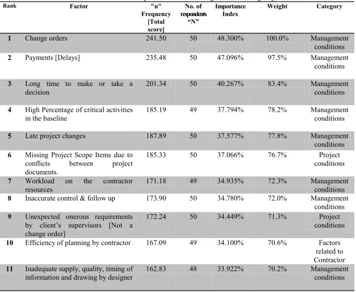
Based on the previous analysis, the most important factors were shown in Table 2 which illustrates the most important 11 factors affect time contingency.

Table 2. The most important factors affecting on time contingency

Rank Factor "n"

Frequency [Total score]

No. of respondents

“N”

Importance

Index Weight Category

1 Change orders 241.50 50 48.300% 100.0% Management

conditions

2 Payments [Delays] 235.48 50 47.096% 97.5% Management

conditions

3 Long time to make or take a

decision 201.34 50 40.267% 83.4% Management conditions

4 High Percentage of critical activities

in the baseline 185.19 49 37.794% 78.2% Management conditions

5 Late project changes 187.89 50 37.577% 77.8% Management

conditions 6 Missing Project Scope Items due to

conflicts between project documents.

185.33 50 37.066% 76.7% Project

conditions

7 Workload on the contractor

resources 171.18 49 34.935% 72.3% Management conditions

8 Inaccurate control & follow up 173.90 50 34.780% 72.0% Management conditions 9 Unexpected onerous requirements

by client’s supervisors [Not a change order]

172.24 50 34.449% 71.3% Project

conditions

10 Efficiency of planning by contractor 167.09 49 34.100% 70.6% Factors related to Contractor 11 Inadequate supply, quality, timing of

information and drawing by designer 162.83 48 33.922% 70.2% Management conditions

3.2.

Projects data

collection

A data gathering form was prepared to collect data from 54 real life building construction projects conducted in Egypt. Data were collected from contractors who are classified by the Egyptian Federation for Construction and Buildings Contractors as a class “A” to confirm the impartiality of conditions and resources between contracting firms of a specific classification. All of these contractors were classified as private companies not public. Ten companies have participated filling the data

gathering form. These data contain residential, commercial and administration buildings projects.

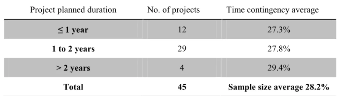
Table 3: Classification of collected data based on planned duration Project planned duration No. of projects Time contingency average

≤ 1 year 12 27.3%

1 to 2 years 29 27.8%

> 2 years 4 29.4%

Total 45 Sample size average 28.2%

4.

Model Development

4.1.

Neural Network and overview

In this paper, Artificial Neural Networks were used as a modeling tool that can enhance current automation efforts in the construction industry. Many applications were previously prepared using artificial neural networks such as Markup estimation, Estimating Resource Requirements at Conceptual Design Stage and many other applications.

There are two types of neural networks. The first type handles classification problems [e.g., into which category of customers targeted by a co mpany does an individual fall]. The second type handles prediction problems [e.g., if certain conditions exist, will a child protective service worker stay or leave his or her job?]. The structure of a neural network model includes an input layer that receive input from the outside world, hidden layers that serve the purpose of creating an internal representation of the problem, and an output layer, or the solution of the problem [17].

Before solving a problem, neural networks must be “trained”. Networks are trained as they examine a smaller portion of the dataset just as they would a normal-sized dataset. Through this training, a network learns the relationships between the variables and establishes the weights between the nodes. Once this learning occurs, a new case can be entered into the network resulting in solutions that offer more accurate prediction or classification of the case [17]

The back-propagation [BP] network is a multilayer feed-forward neural network architecture. This model is used to provide mapping between some input and output quantities by forming a continuous function. In a BP network, no interconnections between neurons in the same layer are permitted. However; each neuron on a layer provides an input to each neuron on the next layer. The BP network uses supervised learning, so the input and output patterns must be both known. In BP, the error calculated at the output of the network is propagated through the layers of neurons in order to update the weights. The architecture of BP model consists of a collection of input units connected to a set of output units

by a set of modifiable connecting weights. BP is the most popular and widely used network learning algorithm [18]. BP was used while preparing the model presented in this paper.

4.2.

Training the Network

All trial models experimented in this research was trained in supervised mode by a back propagation learning algorithm. Inputs were fed to the proposed network model and the outputs were calculated. The differences between the calculated outputs and the actual outputs were then evaluated. The back propagation algorithm develops the input to output mapping by minimizing a root mean square error [RMS] which is expressed by the following equation [19]:

Where: [n] is the number of samples to be evaluated in the training phase.

[Oi] is the actual output related to the sample. [pi] is the predicted output.

This value is being calculated automatically by the Neural Connection 2.0 software. The training process stopped when the value mean square error remains unchanged.

4.3.

Neural Networks software

Neural connections program NC version 2.0 was the software used in this research to develop the neural network model. It requires an IBM compatible 386, 486, or Pentium processor. It can be run on Windows 3.1 or greater and requires a m inimum of 4MB of ram. The program requires 4MB of disk space, a m ouse, and a VGA or SGVA monitor [17].

4.4.

Training the network using NC software:

1. Input data of the Neural Networks was prepared in format of Microsoft Office Excel Comma Separated Values file [.CSV]. These data was created as follows:

1.1. Input fields: it c ontains twelve fields, one for planned duration and eleven fields which present the factors affecting time contingency which previously concluded in the previous sections. Hence, these fields are as follows; [1] Project planned duration in months, [2] No. of change orders, [3] Average of delay in each payment in days, [4] Average duration between submission and approval of change orders, material submittals and inspection requests in days, [5] Percentage of critical activities to the whole activities, [6] No. of changes initiated in last 25% of project actual duration, [7] No. of RFIs [Request for Information], [8] No. of working projects with contractor in the same time including this project, [9] Timing of schedule update, [10] Delay caused by owner -not change orders- in days, [11] Level of time schedule details, [12] Average duration between contractor's RFI submission and response in days.

1.2. Output [Target] field: It contains the actual time contingency in days.

2. Open Neural Connection software.

3. Create three new icons; Input, Multi Layer Perceptron MLP and text as shown in Fig. 1.

Fig. 1. The neural connection icons in NC software.

4. To view the data created in the model click “Input” button then choose “View” from the menu, Fig. 2. The input data includes the project planned duration, values of all factors affecting time contingency and the output is the project delay as illustrated in step [1].

5. Click MLP button then choose “Dialog” from the menu to open the Multi Layer Perceptron dialog box which will be used in the trials and errors practices, Fig. 3.

Fig. 2. Data viewer of Neural connection software

Fig. 3. Multi layer perceptron network dialog box

6. Number of nodes in each layer was written according to the assumptions of each trial.

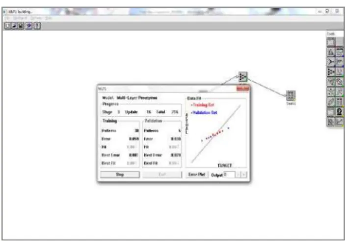
7. Run the program network by clicking “Text” button then choose “Run” from the menu. Fig. 4. shows the running process performed by NC software.

8. NC software automatically shows its report after processing the network data Fig. 5. It shows that the RMS value is 0.661 and the percentage of correct results is 93.75%.

Input

MLP

Fig. 4. NC software runs network.

4.5.

Identify the best structure of the model

To verify this research work, trial and error practices were carried out to conclude the best structure of the model. As mentioned before that the total collected data were Fifty four projects. The model development trials and errors were applied on Forty projects. Five projects were chosen randomly for testing the network. The other nine projects were removed due to extremeness of data.

To confirm that the input data is enough or not, the following test should be done:

 Guideline 1: Number of Training Facts

Minimum Number of Training Facts =2 * [Inputs + Hidden + Outputs]

Maximum Number of Training Facts = 10 * [Inputs + Hidden + Outputs]

This formula suggests that the number of training facts needed is between two and ten times the number of neurons in your network. Where:

• Inputs = 11 factors that determined previously + Planned

duration.

• Outputs = Project delay

• Hidden: A hidden neurons in a hidden layer store the information needed for network to make predications.

There are several ways to determine a good number of hidden neurons. One solution is to train several networks with varying numbers of hidden neurons and select the one that tests best. A second solution is to begin with a small number of hidden neurons and add more while training if the network is not learning. A third solution is starting to get the right number of hidden neurons by using the guideline 2 as follows:

 Guideline 2: Number of Hidden Neurons

Number of Hidden Neurons = [Inputs + Outputs] / 2 = [12 + 1] / 2 = 6.5 ≈ 7 Neurons

Substituting the result of applying the equation ofguideline2 in equations of guideline 1 introduces

•

•

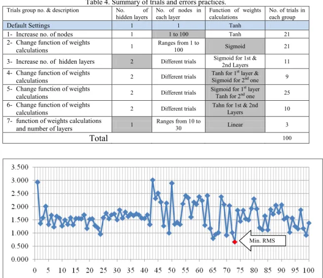
The number of the actual data that obtained is forty. Therefore, this number is satisfactory because it is more than the recommended minimum number that obtained from guideline 1. These two guidelines can help in getting started with first network architecture. Then, after training and testing phases, the changes in the number of hidden layers and the number of hidden neurons will be performed in each layer guided by the percentage of error of the network until the best network is obtained [20]. One hundred trials were applied for model training. These trials were performed in different stages as shown in the Table 4. The gray highlighted cell in each row describes the group of trials. It is divided into five fields; Trials group number and description, number of hidden layers, number of nodes in each layer, function of weights calculations and number of trials in each group. It should be mentioned that the default settings in neural connection 2.0 software is also shown in the first record in Table 4.

It is worth note that the minimum RMS was concluded in the trial number 73. Therefore, it is the recommended structure which should be tested. This structure consists of two layers with function of weights calculations for the first and second layer is Sigmoid and Tahn while no. of nodes in each layer is 50 and 10 nodes respectively. In addition, the mean absolute variance percentage of that structure is (10.41%). Fig. 6 shows the RMS values in each trial.

4.6.

Testing the validity of the model

Table 4. Summary of trials and errors practices. Trials group no. & description No. of

hidden layers No. of nodes in each layer Function of weights calculations No. of trials in each group

Default Settings 1 1 Tanh

1- Increase no. of nodes 1 1 to 100 Tanh 21

2- Change function of weights

calculations 1 Ranges from 1 to 100 Sigmoid 21

3- Increase no. of hidden layers 2 Different trials Sigmoid for 1st & _{2nd Layers} 11

4- Change function of weights

calculations 2 Different trials Tanh for 1

st _{layer &}

Sigmoid for 2nd _one 9

5- Change function of weights

calculations 2 Different trials Sigmoid for 1

st _layer

Tanh for 2nd _one 25

6- Change function of weights

calculations 2 Different trials Tahn for 1st & 2nd Layers 10

7- function of weights calculations

and number of layers 1 Ranges from 10 to 30 Linear 3

Total

Fig. 6. RMS values of each trial.

Then these facts are used to test the ability of network to predict a new output [20]. The model produces the expected project time contingency. Table 5 presents the actual and predicted time contingency which calculated using NC software. It shows that the absolute variance of

time contingency ranges from 0% to 7.5% which is less than previously mentioned mean absolute percentage (10.41%). Therefore the model testing is successfully passed [21].

Table 5. Testing results of neural model. Project

no. Duration Planned [Months]

Time Contingency Variance

Actual Predicted* Value % Absolute %

1 24 25% 25% 0% 0.0% 0.0%

2 20 30% 28% -2% -6.2% 6.2%

3 6 33% 31% -3% -7.5% 7.5%

4 22 27% 28% 1% 2.3% 2.3%

5 18 28% 29% 1% 2.8% 2.8%

* Predicted values are resulted from NC model.

CONCLUSION

The most important factors affecting time contingency includes the following items, ranked by their relative importance; [1] Change Orders, [2] Payment Delays [3] Long time to make or take a d ecision, [4] High

Percentage of critical activities in the baseline, [5] Late project changes, [6] Missing Project Scope Items due to conflicts between project documents, [7] Workload on the contractor resources, [8] Inaccurate control & follow up, [9] Unexpected onerous requirements by client’s supervisor, [10] Efficiency of planning by contractor, [11]

Inadequate supply, quality, timing of information and drawing by designer. Fifty four real life projects were collected from Egypt construction industry. The average time contingency of the collected data was 28%.

Neural networks model was introduced as a management tool that can enhance current automation efforts in the construction industry. ANN model was prepared in order to predict the time contingency of any future project. One hundred trials were applied for model training. The absolute variance of model’s results ranged from 0.0% to 7.5% which is less than previously mentioned mean absolute percentage variance (10.41%). Therefore the model testing is successfully passed.

REFERENCES

[1] Ali Jaafari, “Criticism of CPM for Project Planning Analysis”, J. of Construction Engineering and Management, vol. 110, No. 2, (1984) pp. 222-233. [2] Zayed, T., Mohamed, D., Srour, F., Tabra W. "A

Prediction model for construction project time contingency" Construction Research Congress, (2009) pp. 705–714.

[3] Moonseo Park, and Feniosky Peña-Mora, “Reliability Buffering for Construction Projects”, J. of Construction Engineering and Management, vol. 130, No. 5, (2004) pp. 626-637.

[4] Greg, J. Hoffman; Alfred E. Thai Jr.; Timothy S. Webb; and Jeffery D. “WeirEstimating Performance Time for Construction Projects”, J. of Management in Engineering, vol. 23, No. 4, (2007) pp. 193-199.

[5] Cindy, L. Menches, Awad S. Hanna, and Jeffrey S. Russell, "Effect of Pre-construction Planning on Project outcomes", Construction Research Congress, (2005) pp. 1-10.

[6] Gary, R. Smith, Caryn, M. Bohn. "Small to medium Contractor Contingency and assumption of risk", J. of Construction Engineering and Management, ASCE, March/April, (1999), pp. 101-108.

[7] Hosny, H. “Time Contingency Assessment using Artificial Neural Network” M.Sc. Thesis presented to the college of Engineering and Technology, AASTMT, Cairo branch, Egypt, (2010).

[8] Joao Pedro Couto and Jose Cardoso Teixeira. "The Evaluation of the delays in the Portuguese Construction", CIB World building congress, (2007) pp. 292-301.

[9] K. T. Yeo, "Risks, Classification of Estimates, and Contingency Management", J. of Management in Engineering, ASCE, October, vol. 6, No. 4, (1990) pp. 458-470.

[10] Rifat Sonmez R., Arif Ergin A., and M. Talat Birgonul "Quantitative methodology for determination of cost contingency in international projects" J. of Management in engineering, ASCE, January, Vol.23 No.1, (2007) pp. 35-39.

[11] Soliman, T. “Risk Analysis Methodology for Cost Estimating in Contracting Companies” M.Sc. Thesis presented to the college of Engineering and Technology, AASTMT, Alexandria branch, Egypt, (2005).

[12] Stephen Mak and David Picken, "Using Risk Analysis to Determine Construction Projects Contingencies", J. of Construction Engineering and Management, ASCE, March/April, Vol. 126, No. 2, (2000) pp. 130-136.

[13] Suat Günhan and David Arditi,. "Budgeting Owner’s Construction Contingency", J. of Construction Engineering and Management, ASCE, July, Vol. 133, No. 7, (2007) pp. 492-497. [14] Yaw Frimpong, Jacob Oluwoye, Lynn Crawford.

"Causes of delay and cost overruns in construction of groundwater projects in a developing countries; Ghana as a cas e study", Int. J. of project management, 21, (2003) pp. 321-326.

[15] PMI, “A Guide to the Project Management of Knowledge [PMBOK Guide] Third Edition,”Project Management Institute, PA, USA (2004).

[16] Shash, A. "Factors Considered in tendering decision by top UK Contractors", J. of Construction Management and Economics, 11, (1993) pp. 111-118.

[17] Andrew, S. Quinn, Neural Connection 2.1, University of Texas at Arlington. http://www.und.edu/instruct/aquinn/neural_connect ion.pdf

[18] Hussein, A.A.E., El Thakeb A., Nafie A, Abd Elomngy "Using Artificial Neural Networks in Structural Applications", AL-Azhar University, Cairo, Egypt, November (2005).

[19] Ballard, D.H., "An Introduction to Neural Computation", Massachusetts Institute of Technology (1997).

[20] Azeem, H. “Developing A Neural Networks Model For Supporting Contractors in Bidding Decision In Egypt” M.Sc. Thesis presented to the Faculty of Engineering, Zagazig University, (2008).