UNIVERSIDADE DE SÃO PAULO
INSTITUTO DE RELAÇÕES INTERNACIONAIS
PROGRAMA DE PÓS-GRADUAÇÃO EM RELAÇÕES INTERNACIONAIS
Marketa Maria Jerabek
DO POLITICAL INSTITUTIONS MATTER FOR ECONOMIC PERFORMANCE? A POLITICAL ECONOMY ANALYSIS FOR LATIN AMERICAN COUNTRIES
UNIVERSIDADE DE SÃO PAULO
INSTITUTO DE RELAÇÕES INTERNACIONAIS
PROGRAMA DE PÓS-GRADUAÇÃO EM RELAÇÕES INTERNACIONAIS
DO POLITICAL INSTITUTIONS MATTER FOR ECONOMIC PERFORMANCE? A POLITICAL ECONOMY ANALYSIS FOR LATIN AMERICAN COUNTRIES
Marketa Maria Jerabek
Dissertação apresentada ao Programa de
Pós-Graduação em Relações Internacionais do Instituto de Relações Internacionais da Universidade de São Paulo, para a obtenção do título de Mestre em Ciências – Programa de Pós-Graduação em Relações em Internacionais
Orientadora: Profa. Dra. Adriana Schor
Versão corrigida.
A versão original se encontra disponível na Biblioteca do Instituto de Relações Internacionais e na Biblioteca Digital de Teses e Dissertações da USP, documentos impresso e eletrônico.
Autorizo a reprodução e divulgação total ou parcial deste trabalho, por qualquer meio convencional ou eletrônico, para fins de estudo e pesquisa, desde que citada a fonte.
Catalogação da Publicação
Instituto de Relações Internacionais da Universidade de São Paulo Jerabek, Marketa Maria.
Do Political Institutions Matter for Economic Performance? A Political Economy Analysis for Latin American Countries./ Jerabek, Marketa Maria.; Schor, Adriana. - São Paulo, 2016.
p. 55
Dissertação (Mestrado) – Universidade de São Paulo, 2016.
1. Instituições políticas. 2. Desempenho econômico. 3. América Latina. I. Schor,
People have passed through a very dark tunnel at the end of which there was a light of freedom. Unexpectedly they passed through the prison gates and found themselves in a square. They are
now free and they don’t know
where to go. Václav Havel
5
Abstract
It seems appropriate to compare countries with a similar historical background and a different but comparable level of economic performance in order to make conditional statements. Studies about political institutions and economic performance in Latin American countries were conducted principally in qualitative analyses. The main objective of this study was an attempt based on the political economy to answer the question if different political institutions can explain economic performance in a time series cross section regression analysis. Using 18 Latin American countries for the years 1975-2010 the result of this research permits the conclusion, that political institutions such as political regime, electoral system, federalism on municipal level, partly the ideological polarization degree of executive´s party and the parties in legislature and the stability of a political regime matter for economic performance. Nevertheless, leaping to conclusions about clear causality would be careless and precipitous as the problem of endogeneity of political institutions has not been properly resolved in this research.
Keywords: Political Institutions, Economic Performance, Latin America
Resumo
Parece apropriado comparar países com contextos históricos parecidos e níveis de desempenho econômico diferentes mas comparáveis para poder fazer afirmações condicionais. Pesquisas sobre instituições políticas e desempenho econômico na América Latina foram conduzidas principalmente com metodologias qualitativas. O objetivo principal da presente dissertação foi uma tentativa de responder a questão se as instituições políticas podem influenciar o desempenho econômico nos países da America Latina numa regressão corte transversal de series temporais. Usando 18 países da America Latina para o período de 1975-2010 o resultado deste estudo permite a conclusão que instituições políticas como regime político, sistema eleitoral, federalismo no nível municipal, em parte a distância da ideologia partidária do presidente e dos partidos nas câmaras e da estabilidade do regime político são relevantes para o desempenho econômico. Entretanto, precipitar conclusões sobre uma clara causalidade seria descuidadoso como o problema da endogeneidade das instituições políticas não foi resolvida apropriadamente nesta pesquisa.
6
1. Introduction
Do political institutions matter for economic performance in the case of Latin American countries? In case of affirmation, the subsequent goal of this research consists of ascertaining which political institutions are relevant for economic performance.
The time series cross section analysis of Latin American countries is reasonable. Firstly, as the timeframe of 1975-2010 is shaped by many switches between democratic, semi-democratic and authoritarian regimes in almost all these countries, and thus, providing different political regimes for comparison (see MAINWARING; BRINKS; LIÑÁN, 2008). Only three, Colombia, Venezuela and Costa Rica, of twenty Latin American countries were democratic in 1978 while by 1992 17 of the remaining countries became semi-democratic or democratic (HAGOPIAN; MAINWARING, 2005). Secondly and at the same time as a consequence many Latin American countries are still facing challenges in the democratization process (MILLET, 2009). This current research follows the argument that it is not enough to create subsamples according to the economic development level, at least not for this research about political institutions which are based on cultural and historical pillars. The criteria for the selection of countries, that should be enough different to get enough variation between them and at the same time have enough comparable similarities, depend on the objective of the research. As Latin American countries have a history of colonialism in common and have undergone different political regime changes during the last decades they have a comparable stage in the democratization process, with some country exceptions. This circumstance makes the comparison of political institutions and economic performance among Latin American countries suitable and reliable (same argument in ALBORNOZ; DUTTA, 2007) Further, there exist differences in economic performance between Latin American countries due to
institutional differences (demonstrated for example with the institutional indicator on “doing
7 TABELLINI, 2003, p. 95). Cross-country analyses about political institutions are linked to some difficulties as each country has an individual deep-rooted social, political and economic coinage what makes the direct comparison between the countries political institutions challenging (PEREIRA; TELES, 2009, p. 2). An important conclusion from the conducted research by Pereira and Teles (2009) is that good political institutions matter for economic growth, independent whether they are in an autocracy or democracy. This means that bad political institutions in a democracy can lead to a worse outcome in economic performance then good political institutions in an autocracy. Further, political institutions matter for economic performance in non-consolidated democracies mostly because consolidated democracies have already institutionalized political institutions. Finally, their research expounds the importance of high quality political institutions for the economic performance in countries within a political liberalization process (PEREIRA; TELES, 2009, p. 26).
The research founds on political economy thought claiming that agents such as voters, lobbyists and politicians have different preferences over policies (ACEMOGLU, 2005). Thus, the different distribution of political power among groups in societies leads to different policies across countries. The conflict of interests among various individuals and groups over resource allocation and economic policy results in the formation of different economic institutions (as property rights, entry barriers, etc.) (ACEMOGLU; ROBINSON, 2006). The arrangement of economic institutions is therefore conditioned by the power of political elite groups in a society that shape directly economic institutions. Consequently, the economic policies tend to be beneficial for powerful political groups and individuals rather than for the welfare in a society (ACEMOGLU; JOHNSON; ROBINSON, 2004). Acemoglu and Robinson (2000) argue that societies fail to adopt the best technologies due to institutional failures. Existing powerful interest groups prevent the establishment of new technologies to protect their economic rents and conflicting interests are unified through political institutions into policy decisions (PERSSON; TABELLINI, 2004, p. 85).
8 after the end of colonialism. The newly independent Latin American countries stagnated, especially because of political disorder (NORTH; SUMMERHILL; WEINGAST, 1999).
“The Iberian colonialism failed to create dynamic societies that could independently generate
technological or organizational innovation” (COATSWORTH, 2008, p. 550). Differences in education quality and quantity, differences in the allocation of resources among activities with different productivity levels and the use of different technologies explain only approximately differences in incomes and the different economic performances among countries (ACEMOGLU, 2010). Conforming Acemoglu (2010) institutional explanations appeared beside approaches that emphasize the role of geography and culture for economic performance.
2. Literature
Persson and Tabellini (2000, 2003) have delivered important basic models of political decision-making with implications for economic outcomes and have advanced the political economy research valuably (ACEMOGLU, 2005). Persson, Roland and Tabellini (2007) conclude that proportional representation conducts to more government spending than majoritarian representation in parliamentary democracies. In addition Persson (2005) claims that reforms into parliamentary, proportional and permanent democracy lead to most growth-promoting policies. On the very contrary is embedded Fukuyama’s (2008) argument, without
doing any quantitative research about it, reasoning the impossibility to apply specific political institution features to different countries to obtain better economic outcome. Cultural and historical variety biases predicted economic outcomes of a political institution. Alfano and Baraldi (2008) demonstrated in their panel analysis including Italian regions that a lower degree of proportionality of mixed electoral systems implies a higher regional growth rate.
Additionally, they show that “the impact of corruption on regional growth negatively depends on the degree of proportionality of the mixed electoral systems” (ALFANO; BARALDI,
2008, p. 3). Aboal (2009) goes beyond the distinction of democracy and non-democracy to understand how political institutions influence economic growth. Conforming Aboal (2009) it is not true that democracies always lead to faster growth than dictatorships. The mixed results about the prediction that democracies achieve higher growth than dictatorships (see
9 Furthermore, he argues that proportional representation and majoritarian electoral systems per se do not imply compulsory different economic growth. “This could be one of reasons why
recent empirical works (e.g. PERSSON, 2005) fail to find a clear link between electoral
systems and growth” (ABOAL, 2009, p. 28). Aboal proposes in a further step to include the
distribution of people among classes in order to reveal the effect of proportional and majoritarian electoral systems before making a prediction about the effect of an electoral system on economic growth. These and other papers in this literature all differ in their measure of democracy and choice of specifications, and neither systematically control for the dynamics of GDP nor attempt to address the endogeneity of democratizations (ACEMOGLU; NAIDU; RESTREPO et al., 2014). Acemoglu, Naidu, Restrepo et al. (2014) tested the hypotheses that democracy affects positively economic development and concluded that the effect is significantly positive when using dynamic panel models. Persson and Tabellini do not model GDP dynamics (ACEMOGLU; NAIDU; RESTREPO et al., 2014).
In fact Przeworski and Curvale (2006) analyzed the effect of political institutions in Latin American countries on economic growth, but they did not focus on individual political institutions in a quantitative research. Their main conclusion implies that Latin America in general was left after colonialism without ready-made functioning institutions and therefore fell behind the United States.
As the current state of research shows (see PERSSON; TABELLINI, 2003; ABOAL, 2009; PEREIRA; TELES, 2009) the political causes of the economic performance have been analyzed in cross-country studies, in comparative political economy research, lumping together countries that are delicate for comparison because of their different historical, social and political background. Enikolopov and Zhuravskaya (2007) claim in their research that there are different results between developing and developed countries in relation to the effects of decentralization and other political institutions on economic performance. Therefore, they used subsamples to separate developed countries from developing countries. Meng (2008) applies the same line of argument while studying federalism and its possible impact on economic and social performance in Latin American countries.
10
3. Theories
3.1. Political regime
11 decisions. Growth performance matters for election purposes and populist short-term policies1 as often happening in Latin American countries (DORNBUSH; EDWARDS, 1991) may lose their effects on voting decisions after a series of electoral and economic cycles when the voters begin to analyze skeptically these policies (REMMER, 1991; WEYLAND, 2002). As democratic experiences accumulate the tendency is a shift from populist to more long-term policies favorable to economic growth (GERRING; BOND; BARNDT et al., 2005).
3.2. Electoral systems
To which extent do electoral rules provide incentives to favor special interests or the interests of the broad population? This question is being asked by scholars who analyze whether electoral institutions influence economic performance. This is mostly a function of whether these institutions encourage the candidates to develop personal constituencies or to stimulate their career on collective party results. Actually, the direct interaction between electoral systems and economic performance has not been actively discussed in the literature. The relationship has been rather discussed indirectly via accountability mechanisms, corruption and rent-seeking (PEREIRA; TELES, 2009).
Electoral rules for electing the legislature differ in many dimensions. There are three features of electoral rules: district magnitude, electoral formula and ballot structure (PERSSON; TABELLINI, 2003). “District magnitude simply determines the number of legislators (given
the size of the legislature) acquiring a seat in a typical voting district. One polar case is that all legislators are elected in districts with a single seat, the other that they are all elected in a single, all-encompassing district” (PERSSON; TABELLINI, 2003, p. 22). The translation from votes into seats in the legislature is given by the electoral formula. If citizens vote for individuals or different party lists is determined by the ballot structure.2
The majoritarian system is identified by the first-past-the-post principle which means that the winner takes all the seats of a relevant electoral district. The majoritarian system creates a
“manufactured majority” (NORRIS, 1997), an overrepresentation of the party with the most votes. This means more seats in parliament than votes in the election (ABOAL, 2009) and penalizes minor parties (NORRIS, 1997). Countries with majoritarian systems are often
1 For detailed information about populist policies in Latin American countries see Kaufman and Stallings (1991). 2 In the case of Latin American only Brazil and Panama have open list systems. That is why the ballot structure
12 divided into large number of districts. Proportional electoral systems create a distribution of seats in parliament that is closer to the proportion of votes that each party gained in the elections3 (ABOAL, 2009).
The trade-off between governability and representation is an inherent characteristic of electoral systems (PEREIRA; TELES, 2009). More governability is given in plurality voting systems in single-member districts, while in proportional systems a better representation is provided. Many electoral systems try to attain both objectives - representation and accountability – choosing small multi-member districts or “parallel mixed-member systems, where the proportional seats do not compensate for disproportional outcomes in the
single-member seats” (CAREY; HIX, 2009, p. 3). Such systems give up the pure proportional character in order to increase the accountability (CAREY; HIX, 2009).
Persson and Tabellini (2000, 2006) predict that corruption is higher in a list voting system than in a system where an individual is selected. Further, they found that open list systems
where the party’s order of candidates can be changed lead to better political behavior than closed lists. Persson and Tabellini (2003) also find that the corruption is smaller when individual voting is implemented by the plurality voting system, rather than by using preferential voting or open list in proportional electoral systems. Persson and Tabellini (2006) argue moreover that individual accountability under plurality voting system strengthens the incentives of politicians to satisfy the voters and incentivizes good behavior. Knutsen (2011) on the other side found a positive substantial effect of proportional representation electoral rules on economic growth claiming that proportional electoral systems induce broad-interest policies in relation to education, property rights and free-trade.
Correspondent to Lijphart’s matrix (1991) in figure 1 about the four basic types of democracy, the worst outcome emerges from the combination of presidential system and proportional representation in the legislature; the main characteristic of most of Latin American countries. This combination includes not just gridlock but also the bargaining of the president with disorganized and fragmented parties what has been emphasized by Mainwaring (1993) as well.
3 Throughout the whole research majoritarian electoral system and plurality voting system are utilized
13 Figure 1 - Four basis types of democracy4, adapted from Lijphart (1991, p. 74)
Mainwaring (1993) is right inasmuch as there is a high percentage share of proportional electoral systems in Latin American countries. 50% of the Latin American countries have proportional electoral systems. 27% of these countries have mixed electoral systems, 17% have majoritarian electoral systems and 6% others, visualized in figure 2.
Figure 2 – Electoral systems in Latin America, percentage shares in 2016 (Source: Database of Inter-Parliamentary Union)5
4 PR voting system: Proportional representation voting system, PL voting system: Plurality voting system 5The Inter-Parliamentary Union calculated the percentage shares separately for Central America and South
America. The total of each region is 100%. For figure 2 the values for each electoral system have been summarized, amounting consequently to 200%. Thus, all percentage values have been divided by 2 in order to obtain a total of 100% for the figure.
Majoritarian electoral
system 17%
Proportional electoral
system 50% Mixed
electoral system
27%
14 Nevertheless, the rough global comparison of the four basis types of democracy (MAINWARING, 1993) must be put in a relative perspective when analyzing the data of the Inter-Parliamentary Union in 2016 about the share of proportional, majoritarian and mixed electoral systems in Latin America. 21.05% of the South American countries have majoritarian electoral systems, 15.79% mixed and 63.16% have a proportional electoral system, whereas in Central America 12.5% of the countries have a majoritarian electoral system, 37.5% a mixed, 37.5% proportional systems and 12.5% others.6
3.3. Federalism
Federalism can be defined as a process of political decentralization leading to greater distribution of power and resources between different levels of government (GIBSON, 2004). The principle emerged as a possible solution for intransigent political problems in countries with high levels of ethnic, cultural and language fractionalizations (MENG, 2008). In developing countries decentralization as a public sector reform and linked to democratization with its enhanced voice for citizens in shaping public resource allocation has been supported by academics and practitioners to enhance government performance and economic development (MENG, 2008). Notwithstanding, one has to recognize that little empirical evidence, respectively ambiguous results, have been provided due to the complex diverse mechanisms of federalism in different countries (SMOKE, 2006).
In the context of federalism it is important to mention second generation theories like the
“market-preserving federalism” (WEINGAST, 1995). A market-based approach assumes new
theory of firm behavior by political and economic actors, on all decision levels, as political jurisdictions can be defined as pseudo-firms that provide services (WEINGAST, 1997). Weingast (1997) declares the economic success of England, the United States or Switzerland and recently of China as the legacy of federalism. Competition among subnational governments provides incentives to accomplish economic growth where policies are adapted to local conditions and necessities (WEINGAST, 2006). The second generation of fiscal federalism is rather a positive than normative approach and stresses the importance of local tax revenue. Weingast (2006) argues that there are differences in economic outcomes across
6South America:
http://www.ipu.org/parline-e/ElectoralSystem.asp?LANG=ENG®ION_SUB_REGION=S17&typesearch=1&Submit1=Launch+query
Central America:
15 federal regimes. While Switzerland and the United States, as rich federal countries, and recently China experienced positive effects of federalism, Mexico, Argentina and Brazil had
recorded inferior results. During the 1980’s the debt crises caused changes in economic and
political organization in many Latin American countries where the governments transitioned towards subnational fiscal and administrative management (AVRITZER, 2002). In the early
1980’s the reforms incorporated transfers from the central government to the sub-national level and devolution of resources and responsibilities but the policies failed to consider market-based principles as public choice theory and incentives. The decentralization resulted in random government spending with little regard for budget constraints and generated serious fiscal problems in Argentina, Bolivia, Brazil, Colombia, Ecuador, Mexico and Venezuela in
the early 1990’s. Macroeconomic budget constraints and an overall market-based system of fiscal decentralization were reached after these crises maximizing the efficiency of local public goods (WIESNER, 2003). On the overall effect of decentralization in developing and transition countries has not been reached consensus. In general, some scholars argue that decentralization is beneficial (QIAN; WEINGAST, 1996; MASKIN; QIAN; XU, 2000; GADENNE; SINGHAL, 2014) whereas others disagree (BARDHAN, 2002; CAI; TREISMAN, 2004). Meng (2008) concludes the federalism results often in mixed results in
relation to economic performance in Latin American countries, “especially in the light of the constant tension between centralization and decentralization of central government involvement in the economy and the complexity of ascertaining political capital in a
federation to promote macroeconomic reform” (MENG, 2008, p. 49).
3.4. Party system
As studied by Enikolopov and Zhuravskaya (2007) the effect of fiscal decentralization strongly depends on the strength of national party system and subordination, whether local and state executives are appointed or elected. The relevant theoretical argument has been made by Riker (1964) arguing that party systems influence political incentives of the local governments. In strong national party systems the careers of politicians depend on their party support on local and national level. National governing parties in turn will support local politicians with policies that will not have negative externalities on the overall national
performance. Therefore, local politicians will produce efficient policies. In the 1990 ‘s there
16 (HAGOPIAN, 1998). Strong party systems have been recognized as important actors in the political consolidation and economic reforms in new democracies (HAGGARD; KAUFMAN, 1995). The comparison between Chile and Argentina, which both experienced fiscal decentralization, shows that a strong national party system has positive implications of the effect of fiscal decentralization on economic performance. While in Chile party affiliation is important not only for elections it has experienced better economic outcomes with the decentralization than Argentina, where national political parties are weak (LONDREGAN, 2000; CORRALES 2002). The creation of representative institutions is still a challenging task in new democratic regime in developing countries (ROBERTS; WIBBELS, 1999). Blanchard and Shleifer (2000) illustrated that the same difference can be found between China and
Russia. Whereas China’s decentralization has occurred under control of the communist party, the Russian fiscal decentralization happened with a large political decentralization, which affected negatively the Russian economy.
3.5. Single party versus coalition government
Usually, coalition governments were associated with parliamentarian systems, due to institutional reasons, because presidents do not need to form a legislative majority to take office nor they need a parliamentarian majority to avoid political difficulties. But this view is
changing since the 1980’s as most countries in the Americas have to some degree a multiparty coalition government. However, there is little theoretical discussion about government formation and coalition stability in presidential systems which are in contrast to the existing extensive research about coalition governments in parliamentary systems. Parties in a government in a presidential system are not inevitably veto players7 (the concept comes from the idea of checks and balances in the American constitution see Lijphart, 1984) as they can vote against a bill and remain in government (ALEMÁN; TSEBELIS, 2011). Parties that are ideologically closer to the president should have a higher probability to participate in a government coalition (ALEMÁN; TSEBELIS, 2011). Presidents are concerned about policies, may it be intrinsically or due to electoral reasons and they try to achieve policy outcomes that are close to their own ideologies. Extremist presidents, that defend more leftist or rightist ideologies, are less likely to form cabinets with a majority in congress and produce
7 Distinction between institutional veto players, which are specified by the Constitution, and partisan veto
17 less partisan ministers, (and have for example more technocrats) (ALEMAN; TSEBELIS, 2011). Coalition governments consisting of politicians of different parties have become common in countries like Brazil, Chile and Uruguay (ALEMÁN; TSEBELIS, 2011). In multiparty parliamentary system and presidential system, there exist the possibility of majority coalition formation and a formation of a minority government supported by a majority in parliament. The only difference is that in presidential system there is no option for new elections when a government formation is unsuccessful, as it is the case in parliamentary system when a majority does not support the government. And highly fragmented parliaments favor coalitions in both systems (CHEIBUB; PRZEWORSKI; SAIEGH, 2002). In the existence of a weak congress a president is not required to build a coalition while strong congresses provoke coalition building because in such a situation a president may be concerned about the approval of his policy proposal in congress (ALEMÁN, TSEBELIS, 2011). Tsebelis (1995) bases his analysis about the capacity of policy change on the concept of veto players, which are categorized into institutional (president, chambers) and partisan (partisan) veto players. Veto players are defined as individual or collective actors whose approval is important for a policy change. While Westminster systems, dominant party systems and single-party minority governments consist of only one veto player, federal and presidential systems have several veto players (TSEBELIS, 1995). In multi-party parliamentary and presidential systems the partisan veto players are the parties that are members of a government coalition. An agreement between partisan veto players in a coalition government is not sufficient for a policy change as parliamentary approval is needed. The author argues that the policy stability depends on the characteristics of veto players: their number, their congruence8 and their cohesion9 (TSEBELIS, 1995). In the existence of institutional and partisan veto players the distance between veto players is relevant for policy change, both the distance of institutional veto players and the distance of partisan veto players. Students of political institutions in Latin America argue that divided government (when the president’s party has a minority of seats in a unicameral or bicameral
legislature) leads almost always to gridlock when there is an increased number of parties sharing legislative seats (increased level of party fractionalization congress) (NEGRETTO, 2006). Thus, an extreme multi-party system is not favorable in presidential regimes (MAINWARING, 1993). Nevertheless, most of the Latin American presidential regimes
8 Difference of policy positions among veto players (TSEBELIS, 1995).
18 coexist with multiparty systems and minority presidents were not associated with massive failures of democracies in the region. It can be concluded that it depends on the president’s ability to overcome those formal obstacles, relying for example on informal legislative coalitions. Further, the location of the president’s party in the policy needs to be considered, if the parties care about policy and how deep the ideological polarization is between the
president’s party and the legislative parties (NEGRETTO, 2006).
4. Methodological considerations and model specification
This study is designed to apply a time series cross sectional (TSCS) analysis comprising 18 Latin American countries, namely Argentina, Bolivia, Brazil, Chile, Colombia, Costa Rica, Dominican Republic, Ecuador, El Salvador, Guatemala, Honduras, Mexico, Nicaragua, Panama, Paraguay, Peru, Uruguay, Venezuela for 1975-2010.10 The TSCS is temporal dominant (T>N11) (STIMSON, 1985). Most of the political institutions variables are extracted from the Database of Political Institutions from the World Bank (BECK; CLARKE; GROFF et al., 2001) providing data from 1975 onwards. The economic control variables come from the World Bank Data. A demanding challenge is that an unbalanced TSCS dataset is used. Not all variables are available for all countries during the same period. This leads to a significant loss of the observation number and in some cases to the loss of the number of countries included in the sample. For these reasons different models are estimated to preserve the highest possible number of countries in the sample. Further, it is important to take into account the consideration whether using levels or differences, how to treat serial correlation in the error terms, contemporaneous correlation across units and heteroscedasticity.
In order to account for non-stationarity of real GDP per capita the variable is first differenced and for all the regressions is used the GDP per capita growth as dependent variable.12 Real GDP per capita series in Latin America are non-stationary while GDP per capita growth series are stationary. For each model are conducted heteroscedasticity tests, serial autocorrelation tests, as errors tend to be not independent from a period to the next, and contemporaneous
10Puerto Rico is excluded from the sample as its inclusion might distort the results concerning the fact that it is a
United States territory. The same applies to Cuba. Cuba with its communist regime for the last three decades is not considered to be adequate to study political institutions.
11 T=36, N varies between 14 and 18.
12 The same applies for the variable population growth and gross primary school enrollment, which are also
19 correlation test, as errors tend to be correlated across nations. When heteroscedasticity, first order autocorrelation and contemporaneous correlation are detected ordinary least squares (OLS) is not appropriate.13 Then OLS standard errors shall be substituted by panel-corrected standard errors (PCSEs) as proposed by Beck and Katz (1995)14 and feasible generalized least squares (FGLS) procedure for contemporaneously correlated and panel heteroskedastic errors. The basic model takes the following form15:
∆(log)GDPpercapitac,t = α + ß1Dc,t + ß2*Mc,t + ß3*PLc,t + ß4*MUc,t + ß5*STc,t + ß6*ALLc,t +
ß7*CHc,t + ß8*POLc,t + ß9*∆(log)FRACc,t + ß10*∆(log)PARc,t + ß11*(log)TENSYSc,t +
ß12*CONTROL16 + uc,t + εc,t
5. Variables
Variables Definition Data source
Dependent variable Data World
Bank
∆ (log) real
GDP per
capita17
First differenced log of real GDP per capita (constant 2005 US$), or GDP per capita growth, measuring the economic performance
Independent variables Database of
Political Institutions
13 OLS regression estimates when applied to pooled data are likely to be biased, inefficient and/or inconsistent.
Errors tend to be not independent from a period to the next, correlated across nations, and heteroskedastic (PODESTÀ, 2002).
14 According to Beck and Katz (1995) the best method to treat autocorrelation is via the inclusion of lagged
dependent variables. The parameters are then estimated by OLS and their standard errors by PCSE’s in order to
take into account contemporaneous correlation of the errors and heteroscedasticity. Maddala (1997) however argues that with lagged dependent variables OLS estimators are inconsistent in the presence of serial correlation in erros.
15∆ indicates the first differenced value (to stationarize the variable) of (log) GDP per capita on the left-hand
side of the equation. The between-entity error is expressed in u c, t and the within-entity error in εc, t. 16Control variables are: yrsoffc, WG, GrCapFor, ∆PopGr, ∆GrEnrol, (log)GDPpc65
17 (see DRURY; KREICKHAUS; LUSZTIG, 2006; ENIKOLOPOV; ZHURAVSKAYA, 2007;
20
Democracy, D18 Measuring the political regime. Dummy variable: D=1=Democracy,
D=0=Non-Democracy. The political regime that is the democracy variable causes several challenges as existing democracy indices succumb to measurement errors which lead to doubtful democracy score changes of a country although its institutions do not really change. Democratic and nondemocratic institutions vary considerably in many historical and cultural aspects which turns the analysis about the effect of democracy on economic performance difficult. For these reasons it is used a dichotomous political regime variable.
Military, M19 “Is Chief Executive a military officer?” Dummy variable: M=1=Yes, M=0=No. Due to the fact that many Latin American countries have been military dictatorships at some point in their history the variable M, military, (“Is Chief Executive a military officer?”) from the Political Institutions Database is included as a second dummy variable measuring the political regime.
Plurality, PL20 When legislators are elected through a winner-take all/first part the post rule, the majoritarian electoral system, the variable PL, plurality, assumes the
value=1, when not it equals=0. “1” if there is a competition for the seats in a one-party state (LIEC is 4) (KEEFER, 2012, p. 16). 21
Municipal,
MU22 Federalism (administrative subordination) at the municipal level is measured by MU: no local elections=1, Elections for legislature and appointment of
executive=2, Elections for legislature and the executive=3.
State, ST23 Federalism (administrative subordination) at the state level (or provincial) is
18 Dct ∈ {0,1}, for country c at time t: A country/year observation is coded democratic (Dct = 1) if the Freedom
House status is “Partially Free” or “Free” and its Polity score (see MARSHALL; GURR; JAGGERS, 2014) is positive (ACEMOGLU; NAIDU; RESTREPO et al., 2014). For the case that polity assumes values as -88 or -77 (transitions stage) there is applied the Mainwaring, Brinks and Pérez-Liñán (2008) classification which is the case for El Salvador. The polity classification of -88 for the period 1979-1983 is classified as an authoritarian regime that is why this period is coded nondemocratic (Dct = 0). Semi-democracy classifications of some years are coded as democratic (Dct=1). The same applies to Guatemala for 1985, Honduras 1980-1981, Nicaragua for 1979-1980, Peru 1978-1979, for 2000 Peru is coded as democratic as it is classified as semi-democratic. Mexico has a polity value of 0 for 1988-1993, is classified as a semi-democracy and is coded as democratic (Dct = 1).
19 “If chief executives were described as officers with no indication of formal retirement when they assumed
office, they are always listed as officers for the duration of their term. If chief executives were formally retired military officers upon taking office, then this variable gets a 0 (KEEFER, 2012, p. 5). Otherwise the variable assumes the value 1.
20 The variable measuring proportional electoral system of the database is not applied due to the lack of variance,
as only Chile appears to have a non-proportional electoral system. One has to be aware of the measurement of the variable for the purpose of reality simplification, especially in the moment of interpreting results of plurality.
The chapter with the results summarizes plurality across Latin American countries. A “1” in plurality does not mean that a country has entirely a majoritarian electoral system, a “1” in plurality can occur even when a country
applies in each chamber a different electoral system (as Brazil for example) or has in general a mixed electoral system (as Mexico for example). In this sense the variable plurality is only an approximation.
21 Blank if it is unclear whether there is a competition for seats in a one-party state (LIEC is 3.5) and “NA” is
there is no competition for seats in a one-party state of if legislators are appointed (LIEC is 3 or lower)”
(KEEFER, 2012, p. 16). LIEC Legislative IEC Scale: No legislature: 1
Unelected legislature: 2 Elected, 1 candidate: 3 1 party, multiple candidates: 4
multiple parties are legal but only one party won seats: 5
multiple parties DID win seats but the largest party received more than 75% of the seats: 6 largest party got less than 75%: 7
22 -999 responses and NA are replaced by missing in the dataset (see ENIKOLOPOV; ZHURAVSKAYA, 2007;
21
measured by ST: no local elections=1, Elections for legislature and appointment of executive=2, Elections for legislature and the executive=3.
Allhouse, ALL “Does party of executive control all relevant houses? Does the party of the executive have an absolute majority in the houses that have lawmaking powers? The case of an appointed Senate is considered as controlled by the executive. A senate made up along the lines of ethnic or tribal representation is not controlled by the executive, as these groups nominate their own representatives”
(KEEFER, 2012, p. 8). Dummy variable. The value 1 means that the party of executive controls all relevant houses while the value 0 means that the party of the executive does not have an absolute majority in the houses that have lawmaking powers.
Checks and Lax, CH
Measuring checks and balances. In presidential systems: “CH is incremented by
one:
for each chamber of the legislature unless the president’s party has a majority in
the lower house and a closed list system is in effect
for each party coded as allied with the president’s party and which has an
ideological (left-right-center) orientation closer to that of the main opposition
party than to that of the president’s part” (KEEFER, 2012, p. 19).
Polariz, POL24 The ideological polarization between the president’s party and its allied parties
is measured by polarization: polariz” “is the maximum difference between the chief executive’s party’s value and the values of the three largest government
parties and the largest opposition party” (KEEFER, 2012, p. 19). The variable
takes values of 0 (=the chief executive’s party has an absolute majority in the
legislature), 1 (intermediate difference between the chief executive’s party’s
value and the values of the three largest government party and the largest opposition party, 2 (=maximum difference).
∆(log) FRAC F, fractionalization (log, in order to normalize the data), measuring the party
fractionalization of the parliament. “The probability that two deputies picked at
random from the legislature will be of different parties” (KEEFER, 2012, p. 13).25 First differenced due to unit root.
∆(log) PAR A proxy for the party system (and the strength of institutionalization of the party system) is PAR, party age (log, in order to normalize the data) defined as the average of the ages of the 1st government party, 2nd government party and 1st opposition party.26 First differenced is used due to unit root.
(log)
TENSYS27 “How long has the country been autocratic or democratic, respectively?” (for more information see KEEFER, 2012, p. 18) Political regime stability,
measuring how long a country has been autocratic or democratic, respectively measuring the political regime stability (in years). Aisen and Veiga (2011) found in their research that political instability is associated with lower growth
23 -999 responses and NA are replaced by missing in the dataset (see ENIKOLOPOV; ZHURAVSKAYA, 2007;
KEEFER, 2012).
24 POLARIZ is zero if the chief executive’s party has an absolute majority in the legislature. Otherwise:
POLARIZ is the maximum difference between the chief executive’s party’s value and the values of the three
largest government parties and the largest opposition party See Stasavage and Keefer (2003).
25 NA (in the case of no parliament or no parties in the legislature) and blank spaces (in the case of any
government or opposition party seats) are treated as missing.
26 The variable may be the second-best choice, as the Database of Political Institutions does not provide any
better variable to substitute it.
22
rates of GDP per capita.
Political control variable
Yrsoffc Measures the number of years that the chief officer is in office in year t and country c (DAHL, 1957)
Economic control variables28 Data World
Bank
(log)GDPpc65 GDP per capita from 1965, measuring the initial economic performance. It is used in order to catch the impact of history on economic performance (BARRO, 1991). World Bank data is available since 1960, but only for 1965 there are data available for all relevant countries.
WG29 The world growth (annual %) in order to capture the impact of world economy
on the Latin American economic performance.
GrCapFor30 Gross capital formation (% of GDP)
∆GrEnrol31 Gross primary school enrolment, both sexes (%). First differenced due to unit
root.
∆PopGr32 Population growth (annual %). First differenced due to unit root.
28 Aisen and Veiga (2011) use in their model further variables as the inflation rate, the government size and trade
(as % of GDP). These variables are not used in this research due to the theoretical background on which this research is based on. It is assumed that political institutions affect these variables. For example, Hielscher and Markwardt (2012) found that the quality of political institutions has an impact on inflation. And so is trade policy endogenous (RODRIK, 1992). And Persson, Roland and Tabellini (2007) concluded that political institutions affect the government spending. Thus, this research relies on the logic of Pereira and Teles (2009). They use in their model the average years of schooling and the investment rate as the economic control variables.
29 See POWELL (2015).
30 Definition: Gross capital formation (formerly gross domestic investment) consists of outlays on additions to
the fixed assets of the economy plus net changes in the level of inventories. Fixed assets include land improvements (fences, ditches, drains, and so on); plant, machinery, and equipment purchases; and the construction of roads, railways, and the like, including schools, offices, hospitals, private residential dwellings, and commercial and industrial buildings. Inventories are stocks of goods held by firms to meet temporary or unexpected fluctuations in production or sales, and "work in progress." According to the 1993 SNA, net acquisitions of valuables are also considered capital formation (World Bank:
http://data.worldbank.org/indicator/NE.GDI.TOTL.ZS). See AISEN and VEIGA (2011), PEREIRA and TELES
(2009).
31 Definition: Total enrollment in primary education, regardless of age, expressed as a percentage of the
population of official primary education age. GER can exceed 100% due to the inclusion of over-aged and under-aged students because of early or late school entrance and grade repetition (World Bank:
http://data.worldbank.org/indicator/SE.PRM.ENRR). See AISEN; VEIGA (2011). Pereira and Teles (2009) use
average years of schooling to measure human capital stock. Due to unit root first differenced.
32 Definition: Annual population growth rate for year t is the exponential rate of growth of midyear population
from year t-1 to t, expressed as a percentage. Population is based on the de facto definition of population, which counts all residents regardless of legal status or citizenship--except for refugees not permanently settled in the country of asylum, who are generally considered part of the population of the country of origin (World Bank:
http://data.worldbank.org/indicator/SP.POP.GROW). See AISEN and VEIGA (2011). Due to unit root, first
23
6. Results
6.1. Descriptive statistics
Figure 3 - Timeline of GDP per capita over 1975-2010
The timeline of real GDP per capita depicted in figure 3 reveals a certain time trend with
exponential values since 1990’s for the average value of all sample countries. Peru, El
Salvador, Guatemala, Ecuador, Paraguay, Honduras, Bolivia and Nicaragua have lower values as the average GDP per capita values, whereas countries as Mexico, Venezuela, Argentina, Chile, Costa Rica, Uruguay, Panama, Brazil and Dominican Republic have values above the average over the period of 1975-2010. In the 1980’s an average decline in economic performance can be observed due to negative external shocks, particularly external debt crisis and the second oil shock which is also pictured in figure 4 with the GDP per capita growth evolution over the period 1975-2010. The GDP per capita decline observed in figure 3
in the 1980’s is reflected likewise in figure 4 where most of the countries experienced a decrease in GDP per capita growth. Extreme fluctuations captured until the 1990’s diminished
since then while in the early 2000’s some countries as Uruguay, Argentina and Mexico had
24 Figure 4 – Timeline of GDP per capita growth over the period 1975-2010
This slowdown in the economic growth rate and financial imbalance in the public sector
explain the rise in unemployment and high inflation rates in the 1980’s and much of the
1990’s.33 Simultaneously these two decades were marked by the switch from autocratic regimes to democratic regimes in Latin American countries. Nevertheless, the experiences across the Latin American differed in a significant matter. As Edwards (2007) claims the last
35 years Latin America’s economic performance has been mediocre. Most Latin American
countries implemented marked-oriented reforms during the late 1980’s and early 1990’switch
the intention to reduce fiscal imbalances and inflation, privatize public enterprises develop capital markets, to mention a few of these policy goals, the so-called Washington Consensus (see WILLIAMSON, 1990). Countries as Argentina, Chile and Peru experienced an improved
economic performance in the years following the reforms. The early 2000’s were marked by
traumatic crises. Many countries suffered from balance of payment crises as Brazil in 1999, Argentina in 2001, Uruguay in 2002 and the Dominican Republic in 2003. Mexico experienced repeatedly currency devaluations in 1976, 1982, 1994, Chile in 1982, Brazil in 1999, Argentina in 1989, 2001 and Uruguay in 2002. The next elections were marked by a shift to left oriented governments which were critical of the Washington Consensus. In
33To describe Nicaragua’s situation: “In the late 1970s and the entire 1980s, natural and man-made disasters
25 Bolivia, Ecuador and Venezuela the new political leaders implemented policies that reverted
the reforms of the 1990’s (EDWARDS, 2007). Edwards (2007) predicts that in the future Latin American countries will not experience major improvements in economic performance while some countries might do relatively well and catch up with developed nations. Rodriguez (2004) argues that the economic performance of Latin American countries cannot be understood properly without the analysis of its politics. Since the independence the economic performance of Latin American countries has been influenced by the levels of social, political and economic conflicts.
Figure 5 - Political regime, regime stability and economic performance in Latin America, 1975-2010
Most of the Latin American countries have undergone political regime transitions from autoracies to democracies, except Colombia, Costa Rica and Venezuela34 with no autocratic historical legacies during the analyzed period. The two-sample t test with equal variances for the means of the economic performance values in Latin American autocracies and democracies reveals a clear rejection of the nullhypothesis that the mean difference is zero. The mean value (of 1975-2010) of economic performance in democratic regimes is higher (6267.59, constant 2005 US$) than in autocratic regimes (5104.11, constant 2005 US$). The same test for the second measure of the political regime, military, demonstrates a significant
difference between the economic performance in regimes where the chief executive is a military officer (4932.682, constant 2005 US$) and where not (6285.118, constant 2005 US$). The mean economic performance for 1975-2010 was higher in political regimes
26 without a military officer as a chief executive. The second figure of figure 5 reveals a positive correlation between political regime stability and real GDP per capita.
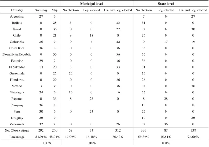
Table 1 - Electoral systems and subnational government/federalism by country, 1975-2010
Table 1 shows that 51.96% of the observations are for non-majoritarian electoral systems and 48.04% for majoritarian electoral systems. The electoral system variable assumes values=1 if the representatives of the House of Representatives or the Senate are elected by majoritarian rule and =0 if not. The variable values present variation among the countries. Few cases where a change from one system to another occurred are observed for the period 1975-2010. Ecuador, El Salvador, Mexico and Venezuela have experienced shifts from one system to
another. “Experience teaches that political change is most difficult when it must confront a
well-structured and robust institutional context” (BLUM, 1997, p. 29). Ecuador switched in 2008 from a proportional to a majoritarian electoral system. El Salvador switched in 1997 from a majoritarian to a proportional electoral system. Mexico switched in 1977 from a proportional to a majoritarian electoral system and Venezuela in 2006 from a proportional to a majoritarian electoral system. Figure 6 illustrates the difference between the average real GDP
Electoral system Subnational government/Federalism
Municipal level State level
Country Non-maj. Maj. No election Leg. elected Ex. and Leg. elected No election Leg. elected Ex. and Leg. elected
Argentina 27 0 7 0 27
Bolivia 0 28 3 0 23 31 0 0
Brazil 0 36 0 0 22 0 6 30
Chile 0 21 8 18 0 26 0 0
Colombia 36 0 0 4 22 0 17 19
Costa Rica 36 0 0 0 36 36 0 0
Dominican Republic 0 36 0 0 36 36 0 0
Ecuador 29 2 0 0 36 36 0 0
El Salvador 13 20 3 0 33 31 0 0
Guatemala 0 25 26 0 0 26 0 0
Honduras 0 29 0 0 26 26 0 0
Mexico 3 33 0 0 36 0 0 36
Nicaragua 24 0 10 0 16 26 0 0
Panama 0 36 8 28 0 8 28 0
Paraguay 36 0 10 0 0
Peru 30 0 0 23 0 27 0 0
Uruguay 26 0 10 0 26
Venezuela 32 4 0 0 26 0 36 0
No. Observations 292 270 58 73 312 336 87 138
Percentage 51.96% 48.04% 13.09% 16.48% 70.43% 59.89% 15.51% 24.60%
100% 100%
27 per capita values over the period 1975-2010. While the average value of 3528.255 (constant 2005 US$) is associated with an majoritarian electoral system and an average value of 3348.151 (constant 2005 US$) with a proportional electoral system. However, the two-sample t test with equal values for the means of the economic performance (between 1975-2010) in proportional and majoritarian electoral systems reveals no significant difference of the mean values (6199.869, constant 2005 US$, for proportional electoral system and 6183.573, constant 2005 US$, for majoritarian electoral system).
Table 1 depicts additional information about subnational government/federalism. 70.43% of the observations are made for elections on municipal legislative and executive level, 16.48% for legislative elections and 13.09% for no elections at all on municipal level. Guatemala is the only country that had no municipal elections at all during 1975-2010. Bolivia, Chile, Colombia, El Salvador , Nicaragua and Panama have undergone changes from a system with no elections at all or only elections on legislative level to elections on legislative level or elections for executives and legislators.
The highest level of subnational government is represented by states/provinces. On the state level 59.89% of the observations show no election on the state level. 15.51% for legislative elections and 24.60% for legislative and executive elections. Argentina, Brazil, Colombia, Panama and Uruguay shifted during 1975-2010 from less state level subnational administration to more, respectively from no elections to legislative elections or from legislative elections to legislative and executive elections (see table 1).
Figure 6 – Subnational administration, electoral system and average real GDP per capita, 1975-2010
2'182.57
3'918.49
3'355.36
2'575.70
4'406.07
5'159.15
3'528.26 3'348.15
0 1000 2000 3000 4000 5000 6000
No local
elections legislatureOnly elected
Legislature and executive
elected
No local
elections legislatureOnly elected
Legislature and executive
elected
Plurality
voting representationProportional voting
Subnational administration: municipal level Subnational administration: state level Electoral system
C
on
st
an
t 2
00
5
U
28 The calculated average real GDP per capita (figure 6) and GDP per capita growth (figure 7) rates for each distinct governmental shape35 on the subnational administration level over the period 1975-2010 point to differences among them.
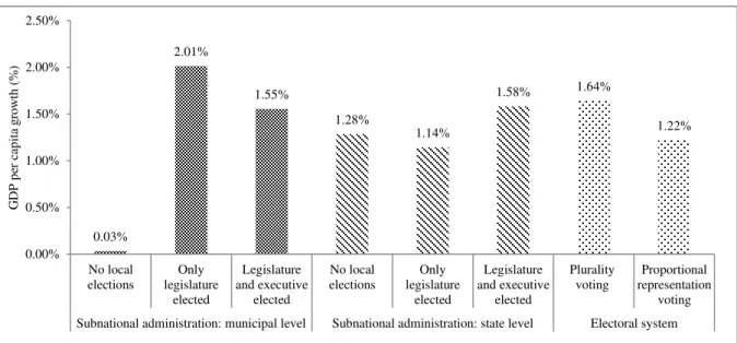
Figure 7 - Subnational administration, electoral system and average GDP per capita growth, 1975-2010
While on the municipal level the highest average real GDP per capita value is observed in the case where only the legislature is elected and the executive is appointed (3918.49 constant 2005 US$, figure 6, or 2.01% GDP per capita growth, figure 7), the highest value of GDP per capita/GDP per capita growth rate on the state level is found where the legislature and executive both are elected (5159.145 constant 2005 US$/1.58% GDP per capita growth). On municipal level the second highest value can be found in the case where both, the legislature and executive are elected (3355.355 constant 2005 US$, figure 6, or 2.01% GDP per capita growth, figure 7) and the lowest value is associated with no local elections (2182.566 constant 2005 US$, figure 6, or 0.03% GDP per capita growth, figure 7).
In order to obtain within country information about the GDP per capita growth before and after a change of governmental shape on subnational administration level (municipal and state/provincial) average GDP per capita growth values are calculated before and after a switch. These results are documented in the consequent figures 8 and 9.
35With 1=no local elections, 2=only legislature elected and executive appointed and 3=both, legislature and
executive elected (both on municipal and state level)
0.03%
2.01%
1.55%
1.28%
1.14%
1.58% 1.64%
1.22%
0.00% 0.50% 1.00% 1.50% 2.00% 2.50%
No local elections
Only legislature
elected
Legislature and executive
elected
No local elections
Only legislature
elected
Legislature and executive
elected
Plurality voting
Proportional representation
voting Subnational administration: municipal level Subnational administration: state level Electoral system
G
D
P
pe
r
ca
pi
ta
g
ro
w
th
(
29 Figure 8 – Average GDP per capita growth and subnational government on municipal level36 - before and after change country comparison
Countries as Bolivia, El Salvador and Nicaragua suffered negative average GDP per capita growth rates when the countries had no local elections on the municipal level. In all three cases a switch from no local elections to elections for the legislature and the executive was accompanied by an increase of average GDP per capita growth rates. Chile, on the other hand, experienced an opposite effect. A higher rate of average GDP per capita growth was observed when no local elections on municipal level were the case. The same observation is made for Colombia and Panama where a higher rate is revealed when the countries had less subnational government, concretely no local elections in Panama and only elections for legislature in Colombia.
36 El Salvador had until 1979 legislative and executive elections on the state level before it switched in 1980 to
no elections at all on state level, which endured for three years. Since 1983 the country established legislative and executive elections on the state level again. For figure 8 the values of GDP per capita growth have been added up from the cases where El Salvador had elections for the executive and legislative, namely from 1975-1979 and from 1983-2010. From this value have been calculated the average of GDP per capita growth.
-12.00% -10.00% -8.00% -6.00% -4.00% -2.00% 0.00% 2.00% 4.00% 6.00%
-2.64%
5.72%
-11.64% -4.21%
2.05% 2.41%
1.87% 1.87% 3.21% 1.92%
1.78% 2.14%
A
ve
ra
ge
G
D
P
pe
r
ca
pi
ta
g
ro
w
th
(
%)
No local elections: municipal level
Only legislature elected: municipal level
30 Figure 9 –Average GDP per capita growth and subnational government on state level - before and after change country comparison
On state level higher average GDP per capita growth rates are detected in Argentina, Colombia and Uruguay after a switch from no local electionsin Argentina and Uruguay and legislature elections in Colombia to elections both for legislature and the executive. In the Brazilian case a higher average GDP per capita growth rate is observed when only the legislature is elected (when compared to the average growth rate in the case of legislature and executive elections). Similarly, Panama experienced a higher average GDP per capita growth rate when it had a lower level of subnational administration, concretely when it had no local elections than when it had only legislature elections.
Figure 10 – (Log) political party age, real GDP per capita and GDP per capita growth
-0.50% 0.00% 0.50% 1.00% 1.50% 2.00% 2.50% 3.00% 3.50% 4.00% 4.50%
-0.27%
2.05%
-0.45% 4.07%
1.83%
1.87% 1.50%
0.99%
1.92%
2.76%
A
ve
ra
ge
G
D
P
pe
r
ca
pi
ta
g
ro
w
th
(
%)
No local elections: state level
Only legislature elected: state level
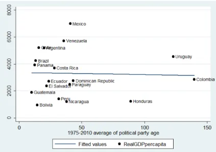
31 Figure 11 – 1975-2010 average political party age and real GDP per capita by country
The scatter plot of political party age and GDP per capita (figure 10) shows a slightly negative correlation between political party age and GDP per capita. It is notable that the majority of Latin American parties are younger than/or 50 years. Only a few countries have political parties with an existence since more than 100 years. Uruguay, Colombia and Honduras show the highest average age of the political parties. Colombia has an average of almost 150 years, and thus has the highest value (figure 11). By contrast, the slight negative correlation in the first figure in figure 10 cannot be confirmed in the second figure where the logarithm of political party age is used and the GDP per capita growth instead of GDP per capita level. Figure 12 illustrates no correlation between the first difference of the (log) of political party and GDP per capita growth.
32 Figure 13 – Fractionalization in legislature and (log) GDP per capita
The correlation between the party fractionalization in the legislature and the (log) real GDP per capita has a negative sign. Only a few observations are found for little fractionalization in legislature. A deeper look into the database provides the information that from 1975-1979 El Salvador and from 1975-1984 Uruguay had no party fractionalization in the legislature. Both countries had during these years a non-democratic political regime. Most of the countries demonstrate a fractionalization in legislature between 0.5 and 0.8. Figure 13 with average real GDP per capita per country and fractionalization in legislature illustrates a stronger negative correlation. While the smallest average fractionalization is observed in Uruguay, followed by Honduras and Mexico, Ecuador has by far the highest average fractionalization value in legislature, followed by Brazil and Bolivia. Figure 14 visualizes no correlation between (log) of fractionalization in legislature and GDP per capita growth.
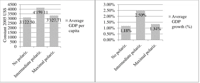
33 Figure 15 – Ideological polarization and average real GDP per capita and GDP per capita growth
Figure 15 depicts the calculated average of real GDP per capita and GDP per capita growth
for the case where the chief executive’s party has an absolute majority in the legislature
(called no polarization in the figure). In this case the average real GDP per capita value is 3122.496, constant 2005 US$, for the period 1975-2010, which is the lowest value among the three groups. The highest average value is 4159.112 (constant 2005 US$) when there is an intermediate difference between the chief executive’s party’s value and the values of the three
largest government parties and the largest opposition party. A maximal ideological polarization is associated with the value 3327.708 (constant 2005 US$) constituting the second highest value. The same ratios between the ideological polarization levels are demonstrated in the figure with average GDP per capita growth rates.
The correlation matrix (see appendix 2) demonstrates clearly that the democracy and military variables are correlated (5% level) with most of the variables measuring other political institutions. But none of the correlation coefficients points out a concern about multicollinearity between these independent variables. Democracy correlates positively and
significantly with real GDP per capita, (log) real GDP per capita and ∆ (log) real GDP per capita while military correlates negatively and significantly with these variables.
3'122.50 4'159.11
3'327.71
0 500 1000 1500 2000 2500 3000 3500 4000 4500
C
on
stan
t 2
00
5
US$
Average GDP per
capita 1.18%
2.50%
1.34%
0.00% 0.50% 1.00% 1.50% 2.00% 2.50% 3.00%
34
6.2. Regression results
Tables 2 and 3 illustrate the regression results from a sample of 15 countries without Argentina, Paraguay and Uruguay (these countries do not have any data available for MU).
Table 4 shows regression results from a sample of 14 countries excluding Argentina, Paraguay and Uruguay due to the aforementioned data lack and additionally Brazil as the data for gross primary school enrollment are not available for this country for the entire period 1975-2010. Table 5 includes all 18 countries as the variables MU, GrEnrol and GrCapFor
have been dropped from the model. Further, the results in table 2 include only political institutions variables. Tables 3, 4 and 5 summarize the results from estimated models with economic control variables.
For all estimated models have been detected serial autocorrelation and heteroskedasticity.37 The significance levels at which the null hypotheses are rejected are: 1 percent, 5 percent and 10 percent (see AISEN; VEIGA, 2011). Each table (2, 3, 4 and 5) presents results from estimated models with random effects with robust standard errors (RE), panel corrected standard errors (PCSE’s) and feasible generalized least squares (GLS). For each method have been estimated two models, one model without first differenced values of (log) party age and (log) fractionalization and one regression with first differenced values of these variables for comparison reasons.38
37 The Wooldridge test for autocorrelation in panel data identified first-order autocorrelation in the estimated
model and the Likelihood-ratio test after estimation for heteroscedasticity in panel data revealed a heteroscedasticity problem in the model. Beck and Katz (1995) argue that the GLS (Generalized least squares) estimates lead to extreme overconfidence, therefore proposing the use of the panel-corrected standard errors (BECK; KATZ, 1995).