REM WORKING PAPER SERIES
Twin Deficits Revisited: a role for fiscal institutions?
António Afonso, Florence Huart, João Tovar Jalles and Piotr Stanek
REM Working Paper 031-2018
March 2018
REM – Research in Economics and Mathematics
Rua Miguel Lúpi 20, 1249-078 Lisboa,
Portugal
ISSN 2184-108X
Any opinions expressed are those of the authors and not those of REM. Short, up to two paragraphs can be cited provided that full credit is given to the authors.
Twin Deficits Revisited: a role for fiscal
institutions?
*
António Afonso$. Florence Huart+ João Tovar Jalles# Piotr Stanek± March 2018
Abstract
We revisit the twin deficit relationship for a sample of 193 countries over the period 1980-2016, using a panel fixed effect (within-group) estimator, bias-corrected least-squares dummy variable, system GMM, and common correlated effects pooled estimation procedures. The analysis accounts also for the existence of fiscal rules in place, their features, and their interaction with the budget balance. In the absence of fiscal rules, the twin deficit hypothesis is confirmed. The size of the estimated coefficient on the budget balance is between 0.68 and 0.79. However, the existence of fiscal rules strongly reduces the effect of budget balance on the current account balance (the coefficient is reduced to 0.1). In fact, the twin deficits relationship does not hold with some specific kinds of rules: debt rules, rules with monitoring of compliance, as well as budget balance rules and debt rules in emerging market economies and lowest income countries, and in the post-crisis period.
Keywords: current account, fiscal balance, fiscal rules, panel data, system GMM
JEL Codes: E62, F32, F41, H87
* The usual disclaimer applies and all remaining errors are the authors’ sole responsibility. The opinions expressed
herein are those of the authors and not of their employers.
$ ISEG – School of Economics and Management, Universidade de Lisboa; REM – Research in Economics and
Mathematics, UECE. UECE – Research Unit on Complexity and Economics is supported by Fundação para a Ciência e a Tecnologia. email: aafonso@iseg.utl.pt.
+ LEM – CNRS (UMR 9221), University of Lille 1, Faculté des Sciences Economiques et Sociales, Villeneuve
d’Ascq. 59655 Cedex France. E-mail: florence.huart@univ-lille1.fr.
# Centre for Globalization and Governance, Nova School of Business and Economics, Campus Campolide, Lisbon,
1099-032 Portugal. UECE – Research Unit on Complexity and Economics. email: joaojalles@gmail.com
± Cracow University of Economics, email: piotr.stanek@uek.krakow.pl. Piotr Stanek gratefully acknowledges
financial support from the Faculty of Economics and International Relations of the Cracow University of Economics in frames of a grant awarded to maintain its research potential.
1. Introduction
Global imbalances along with fiscal consolidation in the aftermath of the Global Financial Crisis and the Great Recession have rekindled the literature about the twin deficits hypothesis: do fiscal deficits cause external deficits? Results from recent empirical studies are not conclusive. The sign and size of the effect of budget balance changes on external balances vary substantially across studies. The introduction of some other relevant factors among the determinants of external balances may reduce much or even counteract the impact of budget deficits on external deficits.
Determining whether the twin deficits hypothesis holds or not is an important issue, because fiscal consolidation may help bring about a reduction in current account deficits if the hypothesis holds for some countries (Bluedorn and Leigh, 2011; Trachanas and Katrakilidis, 2013; Litsios and Pilbeam, 2017) but it is not a panacea if the hypothesis is not confirmed for all countries (Corsetti and Müller, 2016; Algieri, 2013; Afonso, Rault and Estay, 2013). In the latter case, fiscal consolidation could be uneccessarily painful for some countries.
Badinger et al. (2017) investigate the role of fiscal rules in the relationship between fiscal and external balances. Their results confirm the twin deficits hypothesis. They find that fiscal rules do not have any direct effect on the current account balance but their interaction with budget balances reduces the impact of the latter on the current account balance. In particular, debt rules reduce this impact in industrialised countries whereas budget balance rules do so in non-industrialised countries.
In this paper, we want to reconsider the role of fiscal rules in the twin deficits hypothesis. Indeed, the use of fiscal rules has become widespread, but their features and strict enforcement have been diverse across countries (Schaechter et al., 2012). Our work is close to that of Badinger et al. (2017). Our contribution is to revisit the role of fiscal rules by considering other types of fiscal rules, in particular expenditure rules and revenue rules, as well as procedural
rules such as monitoring of compliance with the rule, enforcement of compliance with the rule and the existence of a fiscal council. We also use a large dataset covering 193 countries and a long period of time with recent years (1980-2016).
Our mains findings are as follows: i) The size of the estimated coefficient of the budget balance, in the current account balance estimation, is between 0.68 and 0.79, which is in line with the other recent results, as discussed below in the review of the literature, and confirms the twin deficits hypothesis. ii) The oil balance is the second (along with the budget balance) most robust determinant of the current account (CA) balance, being strongly significant across all specifications. iii) The net foreign assets-to-GDP ratio increases the current account balance only if country fixed effects are omitted. iv) The old age dependency ratio improves the current account balance, thus suggesting that older societies tend to save more. v) The interaction between the existence of fiscal rules and the budget balance is positive and then an improvement in the budget balance leads to an improvement of the current account balance. vi) Expenditure rules have a positive impact on the CA balance, while revenue rules do not have any influence. vii) The existence of an enforcement mechanism of a fiscal rule exerts a positive effect on the current account. All in all, in this case, the main conclusion is that the twin deficit hypothesis no longer holds when there are debt rules, rules with monitoring of compliance, budget balance rules or debt rules in emerging market economies and lowest income countries, and these rules over the post-crisis period.
The remainder of the paper is organized as follows. Section 2 reviews the relevant literature. The following section outlines the theoretical framework. Section 4 details the econometric methodology adopted and presents the underlying data together with some stylized facts. Section 5 discusses our main empirical results and the last section concludes.
2. Literature
In this section we briefly review recent empirical studies on the twin deficits hypothesis. Another related literature deals with the fundamental determinants of the current account. As long as the budget balance belongs to these factors, the results of empirical studies are useful to check the twin deficits hypothesis: a positive statistically significant estimated coefficient on the budget balance variable in an equation where the current account balance is the dependent variable can be interpreted as evidence supporting the hypthesis.1
In previous studies where there was evidence for the twin deficits hypothesis, the coefficient of the relationship between the budget balance and the current account was typically positive and at most 0.30 as pointed out in Corsetti and Müller (2006), Bluedorn and Leigh (2011) or Holmes (2011). In recent works, the estimated coefficient is higher, around 0.50 or 0.60 (Bluedorn and Leigh, 2011; Afonso et al., 2013; Badinger et al., 2017; Litsios and Pilbeam, 2017).
The twin deficits hypothesis used to be rejected in the case of the United States (Müller, 2008; Grier and Ye, 2009). This is because the country is a large and relatively closed economy, and fiscal shocks are not persistent (Corsetti and Müller, 2006). A strong Ricardian effect (increase in private saving) and a crowding-out effect (decrease in private investment) are also found (Kim and Roubini, 2008). These works were based on a VAR analysis.2 However, recent empirical works have tried to address issues related to the existence of structural breaks or regime shifts. Accounting for threshold effects in a cointegration analysis with structural break, Holmes (2011) finds evidence of twin deficits in the case of large public deficits in the U.S. The long run coefficient is 0.42. Nickel and Vansteenkiste (2008) use a panel regression of the
1 For a review of earlier studies on twin deficits, see Algieri (2013), Afonso et al. (2013). For the determinants of
the current account, see Barnes et al. (2010). Table A1 in the Appendix summarizes main findings of the recent literature.
2 In some studies, a public spending shock rather than a government budget deficit shock is considered. On this
current account on several determinants, and a threshold of the government debt-to-GDP ratio. They find that the twin deficit hypothesis holds for 22 indutrialised countries up to a government debt-to-GDP ratio of 90% (80% for 11-euro area countries). Above this threshold, Ricardian equivalence is likely to prevail.
For European countries, and especially countries with large internal and external imbalances (among which Greece, Ireland, Italy, Portugal, and Spain), evidence of twin deficits is mixed: on the one hand, the hypothesis is rejected in Algieri (2013) who uses Granger causality tests; on the other hand, the hypothesis is confirmed for Greece, Portugal and Spain in Trachanas and Katrakilidis (2013) who take into account non linearities (but the primary budget balance is used instead of the overall balance), and in Litsios and Pilbeam (2017) who use a cointegration analysis.
More recently, Badinger et al. (2017) tested for the effect of fiscal rules on the relationship between the budget balance and the current account balance for a panel of 73 countries over the period 1985-2012. Their results confirm the twin deficits hypothesis (with an estimated coefficient around 0.20). The estimated coefficient of the budget balance remains positive and statistically significant when a fiscal rule variable and the interaction of a fiscal rule variable with the budget balance are introduced among regressors. They find that fiscal rules have not any direct effects on the current account balance but they have an indirect negative effect (via the interaction term with the budget balance). This conclusion holds both for budget balance rules and debt rules. However, results differ if the sample is split between industrialised countries and non-industrialised countries: for the former, the twin deficits hypothesis no longer holds with budget balance rules; for the latter, debt rules have not any indirect effects.
3. Theoretical framework
We can recall the standard macro identity:
Y =C+ +I G+X −M (1)
where C is private consumption expenditure, I is private investment, G is government expenditure, X is exports of goods and services, M is imports of goods and services. Hence, private saving S stems from disposable income net of consumption expenditure, and taxes
S=Y−C T− (2)
where T is tax revenue. From (1) and (2) we obtain the current account (CA) balance, the difference between national investment and national saving, which in turn is the sum of private and public saving:
(X −M)=(S −I)+(T −G) (3)
( )
CA= S −I +BUD (4)
and the current account (CA=X-M) balance is related to the budget balance (BUD=T-G) through the difference between private saving and investment. From the above relationships, it is clear that private domestic saving and foreign capital inflow (current account deficit), are in fact the financing sources of both private investment and government budget deficits.
When the government incurs a budget deficit (T-G<0) this may be financed in various ways. For instance, it may be financed by the private sector (S>I), with the government issuing public debt.. Therefore, a government deficit needs not imply a current account deficit. On the other hand, in the presence of a budget surplus and a current account deficit, there would be increases in private investment and/or decreasing private saving (implying S<I).
Under the Ricardian equivalence hypothesis, a decrease in taxes leaves the current account balance unaffected if consumers save more to help pay expected higher future taxes. There could be an effect of the fiscal shock on the current account balance though depending on the degree to which the private sector is liquidity constrained. Note that during recessions, a
budget deficit does not necessarily lead to a current account deficit if the increase in net private saving – due to a fall in private investment – is larger than the decrease in net public saving.
When both the public and the private sectors are in a deficit position, then this will be reflected in a current account deficit (X-M<0). Such an overall shortfall in domestic saving may then be financed by foreign capital inflows, in the form of investments in either domestic public debt or the domestic private sector. This would imply a surplus position in the capital account (KA>0) and the accumulation of foreign reserves, R.
R=CA KA+ (5)
Therefore, if the difference between private saving and investment remains stable, a budget deficit impinges negatively on the current account balance. Overall, this could imply that shocks to the fiscal position may push the current account balance in the same direction, the main point of the twin-deficits argument. However, investment and saving decisions are bound to change given the fiscal deficit, while the effect of fiscal policy on the current account should also depend on the size and the trade exposure of the country. Still evident from equation (4), is that with a given level of saving an increase in the budget deficit will either crowd out private investment or attract additional inflows of capital. In this respect, Corsetti and Müller (2006) show, in a New Open Economy Macroeconomics (NOEM) model, that the twin deficits hypothesis is likely to hold for economies that are more open and with more persistent fiscal shocks. Indeed, they stress the importance of the terms of trade channel that can counterbalance the crowding-out effect of fiscal deficits on private investment.3
In the context of a simple Fleming-Mundell open economy framework, one can recall that with international capital movements and flexible exchange rates, a fiscal expansion could lead to higher interest rates, and in the presence of capital inflows an appreciation of the
3 The increase in prices of domestic goods relative to prices of imported goods raises the rate of return to capital
(much in an economy where the import content of investment is high), and as a consequence, private investment increases (more so if the shock is more persistent and the improvement in the terms of trade lasts longer).
domestic currency may occur which could increase the current account deficit.4 In theory, in the case of perfect capital mobility, with capital flowing among countries to equalise the yield to investors, the current account deficit could increase by exactly the same amount as the budget deficit.5 On the other hand, while a fiscal expansion can drive the current account into deficit, the resulting eventual higher interest rates can push the capital account into surplus. Therefore, the final effect on foreign reserves accumulation is less clear, and depends on the relative sensitivity of international capital flows and on the responsiveness of imports to income. In addition, the appreciation of the currency may improve the current account balance in the short term (through lower import prices) and worsen it with a delay (J-Curve effect). As a result, the contemporaneous impact of a budget deficit may not be a current account deficit.6
The existence of fiscal policy rules may affect the relationship between the budget balance and the current account balance. Twin deficits are unlikely to be observed under a balanced budget rule. However, as discussed in Badinger et al. (2017), there are various (direct and indirect) effects, and the overall effect might be ambiguous. First, if economic agents consider that the existence of fiscal rules reduces uncertainty, favors sound public finances and improves fiscal sustainability, then the need for precautionary saving is reduced. In such a case, we would expect a negative effect of stringent fiscal rules on the current account balance. Second, stricter fiscal rules might bring about lower interest rates. The effect on the current account is uncertain, because there would be a decrease in capital inflows and a depreciation of the currency, but there would also be an increase in domestic spending. Finally, stricter fiscal rules induce stronger Ricardian equivalence and this reduces the effect of the budget balance
4 Dornbusch (1976) showed that the interest rate is a key factor between the adjustments of the domestic economy
and of the current account.
5 With perfect capital mobility, fiscal policy cannot restore the internal balance (Mundell, 1963).
6 In Müller (2008), a dynamic stochastic general equilibrium model is built in order to explain why a positive
government spending shock increases net exports in the case of the United States. His theoretical result stems from a balanced government budget (higher public spending is financed by taxes), a fall in private spending, and a
on the current account balance. Agents expect that the government will correct the budget deficit in the future, if the fiscal rules make it compulsory to do so. Consequently, they save more in order to pay future higher taxes. The decrease in public saving is thus associated with an increase in private saving.
4. Econometric Methodology and Data Issues
4.1 Panel Analysis
We first re-estimate the typical specification used in empirical studies on the twin deficits (Lee et al, 2008; Prat et al., 2010; Lane and Milesi-Ferretti, 2012) using a larger dataset with more cross-sectional observations and a more recent period. Equation (6) below shows our baseline reduced-form empirical model on the determinants of the current account:
, ,
1 2
'
3 4[
*
]
FR BF FR BF
it t i it it it it it it
CA
=
δ
+
γ
+
α
BB
+
α
FI
+
X
α
+
α
FI
BB
+
ε
(6) whereCA
itis the current account balance in percent of GDP,BB
itis the government budgetbalance in percent of GDP,
X
it is a vector of control variables andFI
it is a proxy for fiscal institution, which can comprise of “FR” that is fiscal rules, or “BF” that is budgetary frameworks;δ γ
t,
i denote time and country effects, respectively.ε
itis a disturbance termsatisfying standard conditions of zero mean and constant variance.
The control variables are chosen among fundamental determinants of the current account balance (Lee et al., 2008; Barnes et al., 2010). The latter explain why national saving may exceed or fall short of national investment. Apart from the budget balance (see supra), the relevant variables are the following:
• A higher age dependency ratio is expected to decrease the current account balance. Indeed, a high share of young and old (inactive) people in total population is likely to increase current consumption relative to income. However, an ageing population would
save more today in order to smooth consumption over time. The effect of old age dependency is not settled because saving behavior depends on the pension system. • The population growth rate has a negative effect on the current account balance as long
as it leads to higher consumption (given the increasing share of young people).
• GDP growth is expected to have a negative impact on the current account balance. This effect depends on the import intensity of aggregate demand components. It also depends on whether economic agents perceive the increase in income as being temporary or permanent.
• GDP per capita has a positive impact on the current account balance. In the early stage of economic development, a country needs to borrow abroad because the national saving rate is too low to finance investment. In contrast, rich countries can afford to lend to the rest of the world. This effect can be captured by relative income, which is a country’s GDP per capita relative to the U.S. level.
• Net foreign assets have a positive effect on the current account balance if the country has a net creditor position (it receives net investment income).
• Oil balance is generally preferred to oil prices as a control variable because the latter affect countries differently depending on whether they are producer/exporting or importing countries. A positive oil balance helps improve the current account balance. Equation (6) is first estimated using a panel fixed effect (within-group) estimator — this will serve as our baseline. In some occasions, for sensitivity, country and/or time effects may be dropped. In addition, in some specifications, the interaction term may be absent.
As robustness checks we also employ alternative estimators. More specifically, Equation (6) is also estimated using the bias-corrected least-squares dummy variable (LSDV-C) estimator by Bruno (2005).7
Moreover, the model described above is reduced-form and does not allow making causal statements or even quantifying the clean effect of deflation on fiscal policy aggregates, meaning that the use of instruments is required. While adding covariates present in our vector
X
it partlycorrects for these biases, endogeneity can still arise from other omitted variables (unobserved heterogeneity and selection effects), measurement errors in variables and reverse causality (simultaneity). Since causality can run in both directions, some of the right-hand-side regressors may be correlated with the error term.
In addition, the first-differenced Generalized Method of Moments (GMM) estimator can behave poorly if time series are persistent. Hence, we use the more efficient system GMM estimator that exploits stationarity restrictions. This method jointly estimates Equation (6) in first differences, using as instruments lagged levels of the dependent and independent variables, and in levels, using as instruments the first differences of the regressors (Arellano and Bover, 1995; Blundell and Bond, 1998).8 GMM estimators are unbiased, and compared with ordinary least squares or fixed effects (within-group) estimators, exhibit the smallest bias and variance (Arellano and Bond, 1991). As far as information on the choice of lagged levels (differences) used as instruments in the difference (level) equation, as work by Bowsher (2002) and, more recently, Roodman (2009) have indicated, when it comes to moment conditions (as thus to instruments) more is not always better. The GMM estimators are likely to suffer from
7 Kiviet (1995) used asymptotic expansion techniques to approximate the small sample bias of the standard LSDV
estimator for samples where N is small or only moderately large. Bruno (2005) extended the bias approximation formulas to accommodate unbalanced panels with a strictly exogenous selection rule.
8 We equally tried estimating Equation (6) with a difference GMM estimator but decided against it because the
lagged dependent variable was not significant. Moreover, the tenor of the results is very similar to the system GMM. More specifically, we run the two-step system-GMM estimator with Windmeijer standard errors. The significance of the results is robust to different choices of instruments and predetermined variables.
“overfitting bias” once the number of instruments approaches (or exceeds) the number of groups/countries (as a simple rule of thumb). In the present case, the validity of instruments was examined using Sargan’s test of overidentifying restrictions. Intuitively, the system GMM estimator does not rely exclusively on the first-differenced equations, but exploits also information contained in the original equations in levels.
We also rely on the Pesaran (2006) common correlated effects pooled (CCEP) estimator that accounts for the presence of unobserved common factors by including cross-section averages of the dependent and independent variables in the regression equation, and where the averages are interacted with country-dummies to allow for country-specific parameters. This estimator is a generalization of the fixed effects estimator that allows for the possibility of cross section correlation. Including the (weighted) cross sectional averages of the dependent variable and individual specific regressors is suggested by Pesaran (2006, 2007, 2009) as an effective way to filter out the impacts of common factors, which could be common technological shocks or macroeconomic shocks, causing between group error dependence.
Finally, we inspect the potential role played by outliers in our sample using the Method of Moments that fits the efficient high breakdown estimator proposed by Yohai (1987). In the first stage it takes the S estimator, a high breakdown value method introduced in Rousseeuw and Yohai (1984) applied to the residual scale. It then derives starting values for the coefficient vectors, and on the second stage applies the Huber-type bi-square M-estimator using iteratively re-weighted least squares (IRWLS) to obtain the final coefficient estimates. We also account for outliers and trimmed the sample to extreme values of the dependent variable, which is we exclude similarly to Badinger et al. (2017), current account values above 15 percent of GDP in absolute value.
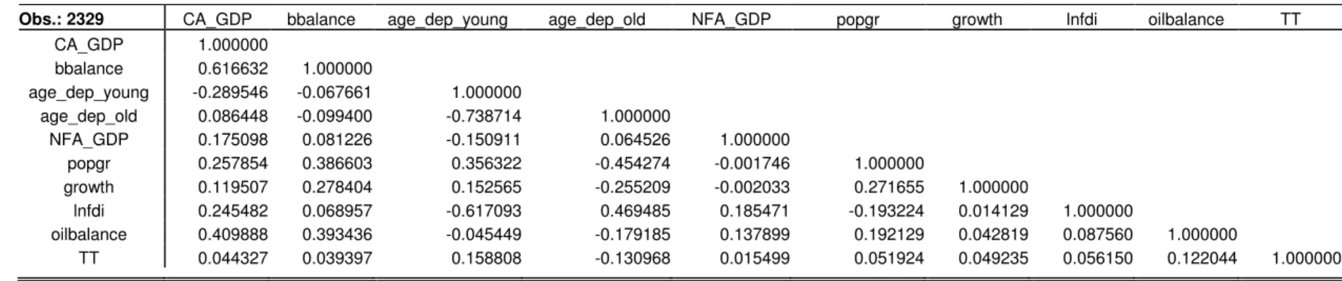
Our sample, for which the macro data come from the IMF World Economic Outlook database, covers 193 countries observed over the period 1980-2016, which yields up to a maximum of 7141 observations. However, the data availability restrains that number to 3858 points for the current account balance (as a share of GDP) and 2894 for the budget balance (with the common sample of 2878 observations). Given the selection of the variables following the procedure proposed by Raftery (1995) the sample size for the baseline model is further reduced to 2329, which is still more than satisfactory for the purposes of our analysis. The detailed descriptive statistics as well as the correlation table are presented in the Appendix (Tables A2 and A3). With the full cross-sectional dimension taken into account, the correlation between the budget balance and the current account balance is very high and relatively insensitive to the selection of the time frame: it assumes values between 0.55 and 0.63.
For individual countries, however, such correlation is not necessarily very robust. This may be illustrated by the inspection of Figure 1, depicting current account balance and budget balance for four selected countries: Canada, France and Japan among developed countries, Bangladesh as an example of a developing one, Poland – a transition economy – and Portugal, a country that suffered from the euro area crisis.
One may notice, that for Canada the relation seems to be quite stable, especially over the period 1990-2010 (with the corresponding correlation coefficient reaching 0.86, whereas for the whole period it is somewhat lower and stands at 0.58). Interestingly, it turns out to be even negative for the pre-NAFTA (pre-1994) period and attains 0.65 since then.
For France in spite of a parallel pattern, the correlation is much weaker than for the whole panel (although still positive) and reaches 0.24. If the French experience is splitted into pre-crisis and post-pre-crisis period, both correlation coefficients are very close to zero (and insignificant). On the other hand, during pre-euro years (until 1998) the correlation was
negative (-0.29) and after the creation of the common currency it turns positive and reaches 0.68.
[Figure 1]
Moreover, the post-crisis period is associated with the return to the twin-deficit pattern in Poland and Portugal, although arguably for different reasons. In Portugal, it seemingly reflected an exogenous external and internal adjustment and the return to close-to-balance values for both current account and budget deficits, whereas in Poland the adjustment is probably driven by a longer run improvement in competitiveness (successful catching-up in productivity). Interestingly, in the pre-crisis period the correlation between the current account and the budget balance for Poland was strongly negative (-0.65), which could be explained by the inflow of Foreign Direct Investment (FDI) (contributing to private investment and allowing for an easy financing of the current account deficits).
Japan exhibits an overall weak relationship between current account balance and budget balance, and some comovement could be observed only until mid-1990s and (to a smaller extent) also in the post-crisis environment. This can be contrasted with the experience of Bangladesh, which has a virtually nil correlation between the current account balance and the budget balance since the crisis, and the highest one (of order of 0.6) for the subperiod between 1980 and 2000. It might suggest that Bangladesh was relatively cut out of international financing until 2000 and enjoys opportunities of international risk sharing (and consumption smoothing) since then, which is exemplified by the increases in FDI inflow in the early 2000s.
Therefore, these differences across individual countries call for an extensive empirical investigation. For instance, the French experience might suggest that implementation of some kind of fiscal rule (related to Stability and Growth Pact) might influence the twin deficit relationship. Thus, a comprehensive set of results will be presented and commented in the following section.
In particular, in order to study the impact of different fiscal rules as well as their specificities and interactions with budget balance on the current account balance we utilize three datasets created by the IMF. The first one was introduced by Schaechter et al. (2012) and its most recent available update, containing data for 96 countries over the period 1985-2015 is discussed in detail by Lledó et al. (2017). The rules are classified according to the following typology: expenditure rules (ER), revenue rules (RR), budget balance rules (BBR) and debt rules (DR). Additionally, we created a dummy variable FR_1, denoting existence of any of these fiscal rules in a given country in a given year. Moreover, the dataset contains information on such features of the rules as existing escape clauses, enforcement procedures or independent monitoring councils or their transparency. In the analysis, we include 65 countries, which had at least one of the rules in place during the period of analysis. Overall, during the 31 years of the timespan at least one rule in place was observed in 1076 cases (on 2015 possible), the most frequent being the budget balance rule (974 cases), followed by debt rule (772 occurrences), expenditure rule (399), the least frequent being the revenue rule (186). Only a handful of countries (Germany, Indonesia, Japan, Malaysia, and Singapore) had at least one rule in place for the entire time span. In all of these cases, it was the balanced budget rule, additionally completed by an expenditure rule (for Germany) and debt rule (in Malaysia). If a given rule was in place, the debt rule was present in a given country for almost 16.5 years, balanced budget rule for 15.7 years, revenue rule for 13.3 years (but it was present only in 13 countries) and expenditure rule for 9.7 years.
The dataset additionally contains information about monitoring, enforcement and escape clause for each type of rules. We utilize this data on somewhat more aggregate level, i.e., if any of the fiscal rules applied in a country had a monitoring of compliance in place, the variable FR_monitor assumes value 1 and zero otherwise. The same is the case for formal enforcement
procedure and escape clauses whereas independent monitoring body and transparency are taken “as they are” from the database.
At least one of these institutions is in place at least for one year in 48 out of 65 countries. The most frequent and relatively persistent is enforcement mechanism, which is in place in 28 countries on average for slightly more than 10 years. Marginally least popular is monitoring (25 countries, on average in place for 9.6 years), Transparency requirements are present in 21 countries, notably on average for the longest period, i.e. for almost 11 years. Independent monitoring body is in place in 22 countries, but as a relatively recent mechanism, its average duration only slightly exceeds 5 years. Finally, some form of escape clause is present in 12 countries, on average for 7.5 years.
Another dataset we utilize was made available by Gupta and Yläoutinen (2014). They analyse fiscal institutional framework, in G-20 economies completed by six low-income countries (Kenya, Mozambique, Myanmar, Uganda, Vietnam and Zambia). In particular, features under scrutiny are fiscal reporting (fr), macro fiscal forecasting (mf), independent fiscal agency (ifa), fiscal objectives (fo), medium term budget framework (mbf), budget execution (be), understanding the scale and scope of the fiscal challenge (understanding), developing a credible fiscal strategy (developing) and implementing the fiscal strategy through the budget process (implementing). Except for ifa, which is present only in 17 out of the 26 countries, all of these institutions are to a smaller or larger extent present in at least 24 countries.
5. Empirical Results
5.1. Baseline
We start with estimating a series of baseline models, where we use the full sample with different combinations of the variables suggested by the literature and we test the robustness of the results to the inclusion of country and time fixe effects (Table 1). The key variable, the budget balance, turns out to be a very important determinant of the current account balance and
this is robust result to different specifications. More precisely, we find that the size of the estimated coefficient on budget balance is between 0.68 and 0.79, which is in line with the other recent results, as discussed above, and confirms the twin deficits hypothesis.
[Table 1]
The other significant determinants include in particular age dependency ratios. Young age dependency exerts the expected and robust effect on the current account: a higher share of youth in population leads to worsening of the current account. The influence of the old age dependency ratio, theoretically being uncertain (potentially increasing either consumption or savings), is empirically found to improve current account balance – thus suggesting that older societies tend to save more. The effect is stronger in terms of absolute value than the one of the young age dependency, but somewhat less robust: in the series of estimates without fixed effects it is significant only if the young age dependency ratio is not included.
The ratio of net foreign assets (NFA) to GDP is positive (as expected) and significant only if country fixed effects are omitted. This might be implied by the fact that NFA tends to change slowly over time and thus country fixed effects could capture its influence.
Population growth, somewhat unexpectedly, exerts a robustly positive, although not very strongly significant, effect on the current account balance (CAB). A one percent increase in population would lead to ca. 0.6 percent improvement of the CAB. This can be contrasted with the lack of influence of economic growth on the CAB in the baseline estimations.
FDI inflow impacts the CAB negatively (as expected) only if country fixed effects are included. This might be implied by the fact that in the whole sample countries enjoying a better CAB possibly attract more FDI on average, whereas the true effect is visible after we control for country specificities.
Oil balance is the second (along with the budget balance) most robust determinant of the CAB: it is strongly significant across all specifications, but quantitatively much stronger
once fixed effects are included. Finally, terms of trade seem to affect the CAB positively despite weak statistical significance.
5.2. Fiscal rules
These baseline results constitute a benchmark for our subsequent, core empirical results. Table 2 presents the results of estimates including the same set of current account determinants as in Table 1, completed by dummies related to the existence of fiscal rules in place and the interaction of each kind of rules with the budget balance. This set of results can be summarized as follows. First, the size and, in some cases the significance, of the incidence of budget balance on the CA falls, which may be, at least to some extent, implied by a smaller sample size due to availability of data on fiscal rules. It is also in line with some theoretical considerations: the existence of fiscal rules may well increase the likelihood of Ricardian equivalence and thus reduce the influence of the budget balance on the current account balance. In this configuration, the impact of one percentage point improvement of budget balance is on average reduced to only 0.1 pp. improvement in the CA.
[Table 2]
The impact of age dependency ratios is also strongly reduced, in terms of both size and significance. However, the impact (if any) of young age dependency remains negative and old age dependency – positive. Interestingly, in this setup the impact of NFA to GDP ratio is positive and significant, of the order 0.03 pp. improvement of the CA balance for each percentage point of higher NFA to GDP ratio. This could be interpreted in terms of net primary income generated by NFA (rate of return on NFA being on average of 3%), which confirms the underlying intuitions.
In this set of results also population growth and economic growth turn out to exert the expected (negative) effect on the CA, the former with elasticity close to 0.9 and the latter of 0.15 (a 1% increase in population worsens the current account to GDP ratio by ca. 0.9%,
whereas a 1% increase in nominal GDP worsens it by 0.15%). Both quantitative and qualitative impact of FDI inflow and oil balance remains unchanged with respect to baseline results including fixed effects (negative in the former case and positive in the latter), terms of trade being systematically insignificant.
As for the direct effects of fiscal rules on the CA and their indirect effects (via their interaction with the budget balance variable), we find that the impact of the existence of fiscal rules in general turns out to be negative (columns 1 and 2 of table 2), but the interaction between the existence of fiscal rules and budget balance is positive. This would suggest that if a fiscal rule is in place, an improvement of budget balance leads to an improvement of the CA. This more than offsets the lack of significance of budget balance incidence on the CA in model (2).
As for expenditure rules (models 3 and 4) its very existence matters and has a positive impact on the CA balance (interaction term is not significant and the coefficient of the budget balance itself does not change dramatically when ER is included in the estimations). On the other hand, revenue rules do not have any influence, neither alone nor as an interaction term. The impact of the balanced budget rule (BBR) (models 7 and 8) is identical to the existence of a fiscal rule in general: the rule alone has a negative impact but including interaction term leads to insignificant coefficients of the budget balance, which is more than offset by the interaction between the BBR and the budget balance. The existence of a debt rule, on the contrary, has a negative impact on the CA and including the interaction term (itself insignificant) makes the BB coefficient insignificant, too. Hence, having fiscal rules in place matters for the relationship between the budget balance and the current account balance, particularly regarding balance budget rules (via an interaction effect). In contrast to Badinger et al. (2017), we thus find that the budget balance rules and debt rules have negative direct effects on the current account balance. In addition, we find that expenditure rules have positive effects whereas revenue rules have not any effects.
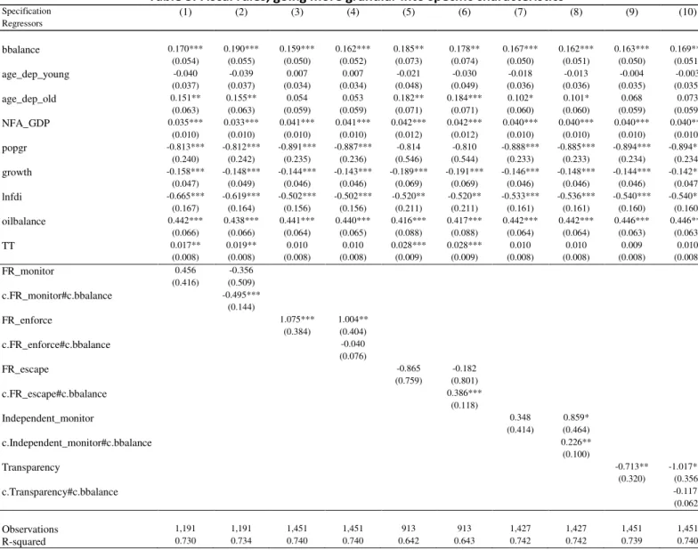
Table 3 presents the results of estimations aiming at a more detailed inspection of specific characteristics of fiscal rules: their monitoring and the independence of this monitoring process, enforcement, and the existence of escape clauses and transparency. This set of results, in terms of macroeconomic determinants (control variables) does not materially differ from the ones presented in Table 2 above, which is implied by a very comparable sample size and country coverage. The only important quantitative change is that the coefficient on budget balance becomes stronger, of the order of 0.16 – 0.2, depending on the specification.
[Table 3]
Monitoring compliance of the fiscal rules in place does not seem to matter directly, but its interaction with the budget balance exerts a negative impact on the current account. This might be interpreted in the following way: monitoring compliance makes fiscal shocks less persistent and ultimately the link between fiscal position and current account becomes a “twin divergence” rather than twin deficit (models 1 and 2 in Table 3). An almost exactly opposite interpretation may be given to the existence of enforcement mechanism of a fiscal rule: such enforcement exerts a positive effect on the current account, without any interaction with the budget balance (models 3 and 4). Unsurprisingly, escape clause exercises the effect directly opposite to monitoring – it is not significant itself, but strengthens twin deficit via interaction term, which is arguably implied by potentially increasing effect of an escape clause on the persistence of the fiscal shocks (models 5 and 6). Independent monitoring does not seem to have a direct influence (model 7), but once the interaction term is included it improves the current account balance both by its existence (more strongly and less significantly) and by the interaction term (less strongly but more significantly), which strengthens the twin deficit pattern. Finally, transparency of a fiscal rule is associated with a worse current account balance,
but the interaction term weakens the relationship between the budget balance and the CA balance.
Table 4 presents the results of the impact of a relatively novel dataset by Gupta and Ylaoutinen (2014) on the relationship between the budget balance and CA. Given a much smaller sample size restrained to G-20 economies, the results that we obtained for this exercise differ from those included in tables 2-3. First, the twin deficit pattern is much stronger (and depending on the exact specification): the direct impact of the budget balance on the CA balance is between 0.36 and as high as 1.13.
Among dependency ratios the one related to the aging of the society is very high and significant (and robust, with coefficients of ca. 0.5) whereas the one related to youth is still negative and significant only at around 10%. The order of value of the NFA impact remains the same, but the significance falls to around 10% as well, whereas population and GDP growth rates are not significant at all.
Interestingly, the FDI and the oil balance keep their size (respectively, around -0.55 and 0.4) and very high statistical significance. Among G-20 countries the terms of trade reveal to be highly significant – an improvement of the terms of trade leads to the improvement of the CA balance with the estimated coefficient of 0.6.
Regarding the fiscal institutional framework, in particular features such as fiscal reporting, macro fiscal forecasting, independent fiscal agency, fiscal objectives, medium term budget framework, budget execution, understanding the scale and scope of the fiscal challenge, developing a credible fiscal strategy and implementing the fiscal strategy through the budget process, our results indicate that they strongly matter for the development of the CA performance and can be summarized as follows. In general, all of the considered aspects of the fiscal institutional setup tend to worsen the CA balance directly and weaken the relationship
between BB and CA (via interaction term). The only exception is “budget execution”, which strongly improves CA balance and has no impact via the interaction with the budget balances.
[Table 4]
5.3. Robustness
Table 5 breaks the sample down into three groups of countries: advanced economies (AE), emerging market economies (EME) and low-income countries (LIC). It turns out that in general the twin deficit behaviour characterizes only AEs (and in specifications without the balance budget rule nor the debt rule) or LICs (only in the specification with expenditure rules). In advanced economies, the young age dependency ratio turns positive, which could be explained by the fact that rich societies tend to save for future education of young generations (are the only ones which can afford it). In addition, the old age dependency is only significant in AEs. The other results on control variables are roughly comparable with the ones presented in tables 2 and 3.
[Table 5]
Interesting, the results are also obtained differently for fiscal rules, per country group. In advanced economies, the mere existence of balanced budget rules and debt rules improves the CA balance. Among the interaction terms, the revenue rule exerts some “twin divergence” effect (albeit not significantly), whereas the balance budget rule and the debt rule strengthen the twin deficit behaviour.
Among EMEs, the revenue rule is associated with a more positive CA balance and weakens the incidence of the budget balance on the current account (via the interaction effect), the balance budget rule worsens the current account and weakens the link between the budget balance and the CA whereas the debt rule does not have any direct impact on current account but also leads to “twin divergence” (again, likely because of decreased persistence of fiscal shocks). Among the LICs, such impact is generally weaker, only balanced budget rules and
debt rules have some negative impact on the CA balance whereas a positive interaction is only visible in the latter case.
Overall, these results confirm that the twin deficit hypothesis does not hold when there are budget balance rules or debt rules in emerging market economies and lowest income countries.
Table 6 reports the results of several robustness checks of the baseline model augmented by the existence of any fiscal rule and its interaction term with budget balance (equivalent to model 2 of table 2) applying different estimators and tools aiming at reducing the impact of outliers. The non-significance of the budget balance coefficient in this specification of the fixed effects panel model is confirmed by LSDV and CCEP estimators as well as for the exclusion of outliers with the absolute value of the current account exceeding 15% of GDP. On the other hand, the system GMM estimator finds the incidence of the budget balance on the CA to be a weak (0.075) but significant at 5%. The outlier-robust estimation (Rousseeuw and Yohai, 1984; Yohai, 1987) finds this key coefficient to be even higher (of the order of 0.2 and significant at 1%). Significance of fiscal rule is detected only by this last method (at a higher significance but also with the opposite sign) and a positive interaction term of the budget balance with any fiscal rule is detected by system GMM, outlier-robust procedure and with the trimmed sample.
Finally, Table 7 applies the same approaches to test the impact of fiscal rules and their interactions with the budget balance on the current account balance (this estimation should be compared to the “even” models of the table 2). It turns out that the direct impact of the fiscal rules as well as their interaction with budget balance are not veritably robust across different methodologies: LSDV does not find any significant impact of any of the rules, system GMM estimation only finds a positive interaction coefficient in the BBR, CCEP finds a positive impact of the ER and weakly positive impact of the interaction term as well as a negative impact of the debt rule both directly and via interaction. Outlier-robust procedure finds all rules
significant as well as their interaction terms (except for debt rule), with BBR and ER having positive impacts on CA, and RR and DR – negative ones. Trimming the outliers out of the sample leads to a positive interaction coefficient of the BBR (confirming the findings of table 2, model 8) and positive and significant effects of ER and its interaction term (which is not in line with our baseline estimates).
[Table 6] [Table 7]
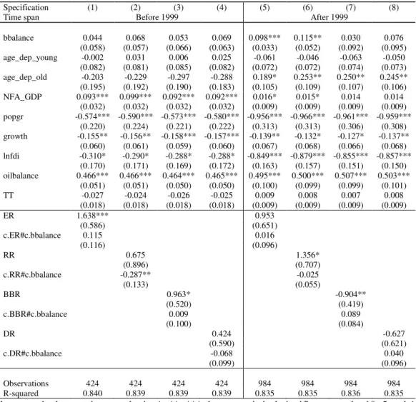
Additionally, we also tested if the results are robust to splitting the sample size after the introduction of the euro (which is equivalent to dividing the time span into two equal subsamples) and testing the twin deficit hypothesis in the pre- and post-crisis environment separately. These results are reported in the appendix – tables A4 and A5. The twin deficit hypothesis is confirmed only in the post-1999 or post-crisis periods, in specifications without the budget balance rule or the debt rule.
6. Conclusion
In this paper we have revisited the twin deficit relationship for a sample of 193 countries over the period 1980-2016, using a panel fixed effect (within-group) estimator, bias-corrected least-squares dummy variable, system GMM, and common correlated effects pooled estimation procedures. Our analysis accounts also for the existence of fiscal rules in place and the interaction of each rule with the budget balance.
Our main findings can be summarized as follows: First, in the baseline estimation without any fiscal rules, the twin deficit hypothesis is confirmed with an estimated coefficient of the budget balance, in the current account balance equation, between 0.68 and 0.79, which is in line with other recent studies. Second, the inclusion of fiscal rules among the regressors reduces the direct effect of the budget balance on the current account balance (the estimated coefficient is reduced to about 0.1). Third, the interaction between the existence of fiscal rules and the budget
balance is positive so that an improvement in the budget balance leads to an improvement of the current account balance. Fourth, expenditure rules have a positive impact on the CA balance, while revenue rules do not have any influence. Fifth, the existence of an enforcement mechanism of a fiscal rule exerts a positive effect on the current account. Finally, we do find evidence of the twin deficit hypothesis when considering budget balance and debt rules, especially in emerging market economies and lowest income countries, and after the great financial crisis. In contrast, and not surprisingly, rules with escape clauses, which attenuate fiscal discipline, reinforce the twin deficits hypothesis.
Overall, our results support the view that fiscal consolidation could be harmful without much benefit in terms of reducing external imbalances in countries that have implemented stringent fiscal rules.
References
1. Afonso, A., Rault, C., & Estay, C. (2013). Budgetary and external imbalances relationship: a panel data diagnostic. Journal of Quantitative Economics, 11(1-2), 45–71. 2. Algieri B. (2013), An empirical analysis of the nexus between external balance and government budget balance: The case of the GIIPS countries, Economic Systems, 37, 233-253. 3. Arellano, M., & Bond, S. (1991). Some Tests of Specification for Panel Data: Monte Carlo Evidence and an Application to Employment Equations. The Review of Economic Studies, 58(2), 277.
4. Arellano, M., & Bover, O. (1995). Another look at the instrumental variable estimation of error-components models. Journal of Econometrics, 68(1), 29–51.
5. Badinger, H., Clairfontaine, A. F. de, & Reuter, W. H. (2016). Fiscal Rules and Twin Deficits: The Link between Fiscal and External Balances. The World Economy, 40(1), 21–35.
6. Barnes S., J. Lawson and A. Radziwill (2010). Current Account Imbalances in the Euro Area: A Comparative Perspective, OECD Economics Department Working Papers No. 826. 7. Beetsma R., M. Giuliodori and F. Klaassen (2008), The effects of public spending shocks on trade balances and budget deficits in the European Union, Journal of the European Economic Association, 6(2-3), 414-423.
8. Bluedorn J. and D. Leigh (2011), Revisiting the Twin Deficits Hypothesis: The Effect of Fiscal Consolidation on the Current Account, IMF Economic Review, 59(4), 582-602. 9. Blundell, R., & Bond, S. (1998). Initial conditions and moment restrictions in dynamic panel data models. Journal of Econometrics, 87(1), 115–143.
10. Bowsher, C. G. (2002). On testing overidentifying restrictions in dynamic panel data models. Economics Letters, 77(2), 211–220.
11. Bruno, G. S. F. (2005). Approximating the bias of the LSDV estimator for dynamic unbalanced panel data models. Economics Letters, 87(3), 361–366.
12. Corsetti G. and G. J. Müller (2006), Twin deficits: squarring theory, evidence and common sense, Economic Policy.
13. Dornbusch, R. (1976). Expectations and Exchange Rate Dynamics. Journal of Political Economy, 84(6), 1161–1176.
14. Easterly, W., & Rebelo, S. (1993). Fiscal policy and economic growth. Journal of Monetary Economics, 32(3), 417–458.
15. Einmahl, J. H., Kumar, K., & Magnus, J. R. (2011). On the choice of prior in Bayesian model averaging. CentER Working Paper, (2011-003).
16. Grier K. and H. Ye (2009), Twin sons of different mothers: The long and the short of the twin deficits debate, Economic Inquiry, 47(4), 625-638.
17. Gupta, M. S., & Yläoutinen, M. S. (2014). Budget Institutions in Low-Income Countries: Lessons from G-20. IMF Working Paper No. 14-164.
18. Holmes M. J. (2011), Threshold cointegration and the short-run dynamics of twin deficit behaviour, Research in Economics, 65, 271-277.
19. Kim S. and N. Roubini (2008), Twin deficit or twin divergence? Fiscal policy, current account, and real exchange rate in the U.S., Journal of International Economics, 74, 362-383. 20. Kiviet, J. F. (1995). On bias, inconsistency, and efficiency of various estimators in dynamic panel data models. Journal of Econometrics, 68(1), 53–78.
21. Lane, P. R., & Milesi-Ferretti, G. M. (2012). External adjustment and the global crisis. Journal of International Economics, 88(2), 252–265.
22. Lee, M. J., Ostry, M. J. D., Prati, M. A., Ricci, M. L. A., & Milesi-Ferretti, M. G.-M. (2008). Exchange rate assessments: CGER methodologies. International Monetary Fund. 23. Litsios I. and K. Pilbeam (2017), An empirical analysis of the nexus between investment, fiscal balances and current account balances in Greece, Portugal and Spain, Economic Modelling, 63, 143-152.
24. Lledó V., S. Yoon, X. Fang, S. Mbaye, &Y. Kim (2017). Fiscal Rules at a Glance. Background Paper. International Monetary Fund, March. Available at:
http://www.imf.org/external/datamapper/FiscalRules/Fiscal%20Rules%20at%20a%20Glance %20-%20Background%20Paper.pdf
25. Magnus, J. R., Wan, A. T. K., & Zhang, X. (2011). Weighted average least squares estimation with nonspherical disturbances and an application to the Hong Kong housing market. Computational Statistics & Data Analysis, 55(3), 1331–1341.
26. Malik, A., & Temple, J. R. W. (2009). The geography of output volatility. Journal of Development Economics, 90(2), 163–178.
27. Müller G. J. (2008), Understanding the dynamic effects of government spending on foreign trade, Journal of International Money and Finance, 27, 345-371.
28. Mundell, R. A. (1963). Capital Mobility and Stabilization Policy Under Fixed and Flexible Exchange Rates. Canadian Journal of Economics and Political Science, 29(4), 475– 485.
29. Nickel C. and I. Vansteenkiste (2008), Fiscal policies, the current account and Ricardian equivalence, ECB Working Paper 935.
30. Pesaran, M. H. (2006). Estimation and Inference in Large Heterogeneous Panels with a Multifactor Error Structure. Econometrica, 74(4), 967–1012.
31. Pesaran, M. H. (2007). A simple panel unit root test in the presence of cross-section dependence. Journal of Applied Econometrics, 22(2), 265–312. Pesaran, M. H. (2009). Weak and strong cross section dependence and estimation of large panels. Keynote speech, 5th Nordic Econometric Meeting, Lund, 29th October.
32. Prat, J., Medina, L., & Thomas, M. A. H. (2010). Current Account Balance Estimates for Emerging Market Economies. International Monetary Fund.
33. Raftery, A. E. (1995). Bayesian Model Selection in Social Research. Sociological Methodology, 25, 111.
34. Roodman, D. (2009). A Note on the Theme of Too Many Instruments. Oxford Bulletin of Economics and Statistics, 71(1), 135–158.
35. Rousseeuw, P., & Yohai, V. (1984). Robust regression by means of S-estimators. Robust and nonlinear time series analysis (pp. 256–272). Springer.
36. Sala-i-Martin, X., Doppelhofer, G., & Miller, R. I. (2004). Determinants of Long-Term Growth: A Bayesian Averaging of Classical Estimates (BACE) Approach. The American Economic Review, 94(4), 813–835.
37. Schaechter A., T. Kinda, N. Budina, & A. Weber, (2012). Fiscal Rules in Response to the Crisis—Toward the “Next-Generation” Rules. A New Dataset. IMF Working Paper WP/12/187.
38. Trachanas E. and C. Katrakilidis (2013), The dynamic linkages of fiscal and current account deficits: New evidence from five highly indebted European countries accounting for regime shifts and asymmetries, Economic Modelling, 31, 502-510.
39. Yohai, V. J. (1987). High Breakdown-Point and High Efficiency Robust Estimates for Regression. The Annals of Statistics, 15(2), 642–656.
TABLES
Table 1. Baseline, alternative specifications, different country and time effects, all countries
Specification (1) (2) (3) (4) (5) (6) (7) (8) (9) (10) (11) (12) Regressors Bbalance 0.786*** 0.747*** 0.780*** 0.740*** 0.686*** 0.694*** 0.699*** 0.692*** 0.717*** 0.721*** 0.726*** 0.719*** (0.133) (0.147) (0.139) (0.147) (0.173) (0.176) (0.177) (0.176) (0.171) (0.173) (0.174) (0.174) age_dep_young -0.097*** -0.100*** -0.127*** -0.125*** -0.124*** -0.121*** (0.017) (0.017) (0.027) (0.027) (0.031) (0.031) age_dep_old 0.273*** 0.020 0.197*** 0.024 0.172*** 0.198*** 0.243*** 0.205*** 0.215*** 0.196*** 0.123* 0.201*** (0.064) (0.083) (0.064) (0.083) (0.055) (0.066) (0.065) (0.063) (0.068) (0.074) (0.067) (0.069) NFA_GDP 0.014*** 0.012*** 0.013*** 0.012*** 0.000 0.009 0.016 0.009 0.003 0.009 0.012 0.009 (0.003) (0.003) (0.003) (0.003) (0.009) (0.011) (0.011) (0.011) (0.008) (0.011) (0.011) (0.011) popgr 0.519 0.668* 0.585* 0.687* 0.632* 0.663** 0.665** 0.666** 0.606** 0.634** 0.635** 0.637** (0.364) (0.373) (0.357) (0.374) (0.343) (0.327) (0.330) (0.329) (0.300) (0.286) (0.287) (0.288) growth -0.013 -0.043 -0.057 -0.045 -0.039 -0.014 -0.020 -0.012 -0.016 0.008 0.010 0.009 (0.080) (0.090) (0.091) (0.091) (0.072) (0.075) (0.078) (0.075) (0.082) (0.087) (0.088) (0.087) lnfdi 0.192** 0.513*** 0.189** -0.643*** -0.438*** -0.672*** -0.558*** -0.557*** -0.592*** (0.094) (0.071) (0.093) (0.138) (0.113) (0.138) (0.159) (0.158) (0.160) oilbalance 0.105*** 0.081*** 0.095*** 0.082*** 0.440*** 0.448*** 0.451*** 0.450*** 0.448*** 0.451*** 0.448*** 0.450*** (0.020) (0.021) (0.022) (0.021) (0.041) (0.039) (0.041) (0.040) (0.041) (0.040) (0.041) (0.041) TT 0.002 0.010** 0.010* 0.005 0.008 0.006 (0.006) (0.005) (0.006) (0.006) (0.006) (0.006) Country effects NO NO NO NO Yes Yes Yes Yes Yes Yes Yes Yes
Time effects NO NO NO NO No No No No Yes Yes Yes Yes
Observations 2,529 2,350 2,329 2,329 2,529 2,350 2,329 2,329 2,529 2,350 2,329 2,329 R-squared 0.463 0.493 0.477 0.497 0.712 0.723 0.720 0.724 0.723 0.734 0.732 0.734
Note: robust standard errors in parenthesis. *, **, *** denote statistical significance at the 10, 5 and 1 percent levels, respectively.
Table 2. adding fiscal rules – general with all countries Specification (1) (2) (3) (4) (5) (6) (7) (8) (9) (10) Regressors bbalance 0.116*** -0.031 0.098*** 0.082*** 0.104*** 0.099*** 0.110*** -0.051 0.110*** 0.069 (0.030) (0.060) (0.030) (0.031) (0.031) (0.038) (0.031) (0.063) (0.031) (0.060) age_dep_young -0.038 -0.057* -0.044 -0.046 -0.037 -0.037 -0.030 -0.053* -0.030 -0.035 (0.032) (0.033) (0.032) (0.032) (0.032) (0.032) (0.031) (0.033) (0.031) (0.032) age_dep_old 0.052 0.084 0.066 0.083 0.101* 0.101* 0.077 0.114* 0.077 0.072 (0.060) (0.060) (0.059) (0.059) (0.060) (0.060) (0.060) (0.060) (0.059) (0.059) NFA_GDP 0.034*** 0.033*** 0.034*** 0.033*** 0.033*** 0.033*** 0.033*** 0.032*** 0.033*** 0.032*** (0.009) (0.009) (0.009) (0.009) (0.009) (0.009) (0.009) (0.009) (0.009) (0.009) popgr -0.889*** -0.884*** -0.878*** -0.885*** -0.885*** -0.884*** -0.891*** -0.883*** -0.887*** -0.880*** (0.217) (0.215) (0.221) (0.220) (0.221) (0.221) (0.219) (0.216) (0.219) (0.219) growth -0.150*** -0.139*** -0.153*** -0.155*** -0.153*** -0.152*** -0.150*** -0.136*** -0.151*** -0.148*** (0.043) (0.043) (0.043) (0.043) (0.043) (0.044) (0.043) (0.043) (0.043) (0.043) lnfdi -0.600*** -0.606*** -0.562*** -0.575*** -0.585*** -0.585*** -0.594*** -0.591*** -0.595*** -0.595*** (0.143) (0.140) (0.147) (0.148) (0.143) (0.143) (0.144) (0.139) (0.143) (0.142) oilbalance 0.435*** 0.438*** 0.431*** 0.434*** 0.436*** 0.436*** 0.437*** 0.439*** 0.432*** 0.435*** (0.065) (0.065) (0.067) (0.067) (0.067) (0.067) (0.066) (0.065) (0.065) (0.066) TT -0.005 -0.007 -0.004 -0.005 -0.005 -0.005 -0.005 -0.007 -0.005 -0.006 (0.006) (0.006) (0.007) (0.007) (0.007) (0.007) (0.007) (0.006) (0.006) (0.006) FR_1 -1.155*** -0.670* (0.367) (0.361) c.FR_1#c.bbalance 0.187*** (0.060) ER 0.850** 1.102** (0.401) (0.464) c.ER#c.bbalance 0.118 (0.079) RR 0.084 0.119 (0.468) (0.470) c.RR#c.bbalance 0.018 (0.049) BBR -0.769** -0.225 (0.375) (0.372) c.BBR#c.bbalance 0.211*** (0.063) DR -1.006*** -0.804** (0.385) (0.401) c.DR#c.bbalance 0.069 (0.072) Observations 1,408 1,408 1,408 1,408 1,408 1,408 1,408 1,408 1,408 1,408 R-squared 0.757 0.759 0.756 0.756 0.755 0.755 0.756 0.759 0.757 0.757
Note: Note: robust standard errors in parenthesis. *, **, *** denote statistical significance at the 10, 5 and 1 percent levels, respectively. “FR_1” if a country has at least one fiscal rule; “ER” = expenditure rule in place; “RR” revenue rule in place; “DR” = debt rule in place; “BBR” = budget balance rule in place
Table 3. Fiscal rules, going more granular into specific characteristics Specification (1) (2) (3) (4) (5) (6) (7) (8) (9) (10) Regressors bbalance 0.170*** 0.190*** 0.159*** 0.162*** 0.185** 0.178** 0.167*** 0.162*** 0.163*** 0.169*** (0.054) (0.055) (0.050) (0.052) (0.073) (0.074) (0.050) (0.051) (0.050) (0.051) age_dep_young -0.040 -0.039 0.007 0.007 -0.021 -0.030 -0.018 -0.013 -0.004 -0.003 (0.037) (0.037) (0.034) (0.034) (0.048) (0.049) (0.036) (0.036) (0.035) (0.035) age_dep_old 0.151** 0.155** 0.054 0.053 0.182** 0.184*** 0.102* 0.101* 0.068 0.073 (0.063) (0.063) (0.059) (0.059) (0.071) (0.071) (0.060) (0.060) (0.059) (0.059) NFA_GDP 0.035*** 0.033*** 0.041*** 0.041*** 0.042*** 0.042*** 0.040*** 0.040*** 0.040*** 0.040*** (0.010) (0.010) (0.010) (0.010) (0.012) (0.012) (0.010) (0.010) (0.010) (0.010) popgr -0.813*** -0.812*** -0.891*** -0.887*** -0.814 -0.810 -0.888*** -0.885*** -0.894*** -0.894*** (0.240) (0.242) (0.235) (0.236) (0.546) (0.544) (0.233) (0.233) (0.234) (0.234) growth -0.158*** -0.148*** -0.144*** -0.143*** -0.189*** -0.191*** -0.146*** -0.148*** -0.144*** -0.142*** (0.047) (0.049) (0.046) (0.046) (0.069) (0.069) (0.046) (0.046) (0.046) (0.047) lnfdi -0.665*** -0.619*** -0.502*** -0.502*** -0.520** -0.520** -0.533*** -0.536*** -0.540*** -0.540*** (0.167) (0.164) (0.156) (0.156) (0.211) (0.211) (0.161) (0.161) (0.160) (0.160) oilbalance 0.442*** 0.438*** 0.441*** 0.440*** 0.416*** 0.417*** 0.442*** 0.442*** 0.446*** 0.446*** (0.066) (0.066) (0.064) (0.065) (0.088) (0.088) (0.064) (0.064) (0.063) (0.063) TT 0.017** 0.019** 0.010 0.010 0.028*** 0.028*** 0.010 0.010 0.009 0.010 (0.008) (0.008) (0.008) (0.008) (0.009) (0.009) (0.008) (0.008) (0.008) (0.008) FR_monitor 0.456 -0.356 (0.416) (0.509) c.FR_monitor#c.bbalance -0.495*** (0.144) FR_enforce 1.075*** 1.004** (0.384) (0.404) c.FR_enforce#c.bbalance -0.040 (0.076) FR_escape -0.865 -0.182 (0.759) (0.801) c.FR_escape#c.bbalance 0.386*** (0.118) Independent_monitor 0.348 0.859* (0.414) (0.464) c.Independent_monitor#c.bbalance 0.226** (0.100) Transparency -0.713** -1.017*** (0.320) (0.356) c.Transparency#c.bbalance -0.117* (0.062) Observations 1,191 1,191 1,451 1,451 913 913 1,427 1,427 1,451 1,451 R-squared 0.730 0.734 0.740 0.740 0.642 0.643 0.742 0.742 0.739 0.740
Note: Note: robust standard errors in parenthesis. *, **, *** denote statistical significance at the 10, 5 and 1 percent levels, respectively. “monitor” = at least one of the rules in place monitor compliance exist; “enforce” = at least one of the rules in place formal enforcement procedure exist; “escape” at least of the rules in place escape clause exist.
Table 4. Budget Institutions (data from Gupta and Ylaoutinen, 2014 IMF WP) Specification (1) (2) (3) (4) (5) (6) (7) (8) (9) Regressors bbalance 0.720*** 0.567*** 0.361*** 0.414* 0.670*** 0.581* 0.544*** 0.731*** 1.128*** (0.167) (0.132) (0.098) (0.232) (0.145) (0.310) (0.126) (0.175) (0.333) age_dep_young -0.121 -0.125 -0.134* -0.149* -0.123 -0.143* -0.124 -0.127 -0.127 (0.081) (0.082) (0.082) (0.083) (0.081) (0.083) (0.082) (0.081) (0.082) age_dep_old 0.465*** 0.480*** 0.494*** 0.520*** 0.524*** 0.489*** 0.467*** 0.484*** 0.476*** (0.107) (0.108) (0.108) (0.109) (0.107) (0.115) (0.109) (0.107) (0.110) NFA_GDP 0.032* 0.032 0.033 0.031 0.033* 0.029 0.033* 0.031 0.031 (0.020) (0.020) (0.021) (0.021) (0.020) (0.021) (0.020) (0.020) (0.021) popgr -0.970 -0.887 -0.737 -0.668 -0.968 -0.764 -0.877 -0.909 -0.936 (0.734) (0.745) (0.760) (0.775) (0.732) (0.784) (0.745) (0.737) (0.758) growth -0.081 -0.094 -0.101 -0.099 -0.076 -0.085 -0.093 -0.079 -0.083 (0.071) (0.073) (0.076) (0.078) (0.070) (0.074) (0.073) (0.071) (0.072) lnfdi -0.554** -0.561** -0.555** -0.546** -0.542** -0.538** -0.558** -0.555** -0.533** (0.264) (0.267) (0.268) (0.265) (0.264) (0.273) (0.267) (0.264) (0.268) oilbalance 0.407*** 0.421*** 0.424*** 0.441*** 0.409*** 0.436*** 0.414*** 0.416*** 0.419*** (0.045) (0.046) (0.049) (0.047) (0.046) (0.048) (0.047) (0.046) (0.047) TT 0.059*** 0.063*** 0.066*** 0.069*** 0.062*** 0.066*** 0.061*** 0.061*** 0.064*** (0.011) (0.011) (0.011) (0.011) (0.011) (0.011) (0.011) (0.011) (0.011) fr -9.648*** (2.196) c.fr#c.bbalance -0.378*** (0.103) mf -4.675*** (1.065) c.mf#c.bbalance -0.277*** (0.083) ifa -5.065*** (1.205) c.ifa#c.bbalance -0.176** (0.080) fo -4.249*** (1.246) c.fo#c.bbalance -0.119 (0.165) mbf -6.775*** (1.495) c.mbf#c.bbalance -0.416*** (0.104) be 26.321*** (7.517) c.be#c.bbalance -0.243 (0.215) understanding -5.786*** (1.289) c.understanding#c.bbalance -0.314*** (0.089) developing -8.317*** (1.914) c.developing#c.bbalance -0.446*** (0.128) implementing -56.668*** (15.308) c.implementing#c.bbalance -0.664*** (0.230) Observations 537 537 537 537 537 537 537 537 537 R-squared 0.796 0.793 0.789 0.788 0.796 0.788 0.793 0.795 0.792
Note: Note: robust standard errors in parenthesis. *, **, *** denote statistical significance at the 10, 5 and 1 percent levels, respectively. “fr”=fiscal reporting; “mf”=macro fiscal forecasting; “IFA”=independent fiscal agency; “fo” fiscal objectives; “MBF” medium term budget framework; “be” budget execution; “understanding”=understanding the scale and scope of the fiscal challenge; “developing” = developing a credible fiscal strategy; “implementing” = implementing the fiscal strategy through the budget process.